Constructing U.K. Core Inflation

Abstract

The recent volatile behaviour of U.K. inflation has been officially attributed to a sequence of “unusual” price changes, prompting renewed interest in the construction of measures of “core inflation”, from which such unusual price changes may be down-weighted or even excluded. This paper proposes a new approach to constructing core inflation based on detailed analysis of the temporal stochastic structure of the individual prices underlying a particular index. This approach is illustrated using the section structure of the U.K. retail price index (RPI), providing a number of measures of core inflation that can be automatically calculated and updated to provide both a current assessment and forecasts of the underlying inflation rate in the U.K.

1. Introduction

The behaviour of inflation in the U.K. since 2007, and particularly after the “credit crunch” of 2008, has been extremely volatile. After a period of relatively high values, annual inflation dipped alarmingly to display several months of negative inflation between March and October 2009, prompting fears of deflation, before rebounding quickly to reach levels well above the Bank of England’s Monetary Policy Committee’s (MPC) target range. This behaviour forced the Governor of the Bank to send a sequence of letters to the Chancellor of the Exchequer (required under the Bank’s remit of independence) explaining this inflation performance. These letters, beginning in April 2007, characterize the high inflation as primarily a consequence of temporary factors: “the MPC’s assessment is that much of the current high level of inflation can be attributed to the increase in VAT in January 2010, past rises in oil prices and the continued pass-through of higher import prices following the depreciation of sterling since mid-2007. The MPC’s central judgement remains that these effects will prove to have a temporary impact on inflation” (August 2010); “the current elevated rate of inflation largely reflects a number of temporary influences” (November 2010); and “three factors can account for the current high level of inflation: the rise in VAT relative to a year ago, the continuing consequences of the fall in sterling in late 2007 and 2008, and recent increases in commodity prices, particularly energy prices. Although one cannot be sure, prices excluding the effects of these factors would probably have increased at a rate well below the 2% inflation target” (February 2011). A later letter (November 2011) continues this theme: “the current high inflation reflects the increase in the standard rate of VAT earlier this year, and previous steep increases in import and energy prices, including recent domestic utility price rises. In the absence of those temporary factors, it is likely that inflation would have been below … target”. 1

While the inflation experiences of some other industrialized countries may not have been quite so extreme, the impact of “unusual” price changes in various sectors of the advanced economies has created a continued interest in measuring “core” inflation. Such a concept is not new, of course, for it seems to have first surfaced during the mid-1970s, when the major economies were being buffeted by a sequence of oil price shocks, with the initial reference to it appearing to be Gordon [1], followed shortly after by a more detailed exposition by Eckstein [2]. Over the last decade or so core inflation has frequently been discussed, and several measures of it proposed, as more central banks have adopted inflation targets. Notable surveys of the concept and its various operational measures are Mankikar and Paisley [3], Rich and Steindel [4], Silver [5] and Wynne [6], all of whom may be consulted for extended discussion, empirical comparisons and historical assessment.

There are two broad approaches to defining and measuring core inflation. An approach that was particularly popular during the second half of the 1990s may be termed the economic theory or model-based approach, its most notable proponents being Quah and Vahey, who defined core inflation to be the component of measured inflation that has no medium to long-run impact on real output, motivating this definition by the assumption of a vertical long-run Phillips curve [7]. Their measure is constructed by placing long-run coefficient restrictions on a bivariate non-cointegrated vector autoregressive VAR system for output and inflation. Although technically sophisticated, it seems that measures of core inflation computed in this way may be sensitive to the variety of, on the face of it, seemingly innocuous auxiliary assumptions that necessarily have to be made when engaging in VAR modelling.

The alternative is the statistical approach, which generally combines index number theory for aggregating the individual prices to form an overall price index with various measures for determining the weights employed in the aggregation. Rather than use the traditional expenditure shares directly as weights, these shares may be adjusted by using factors such as price volatility or forecasting ability, or these factors may simply replace the expenditure shares as weights. A traditional approach is to give either or both energy and food prices zero weights, so defining the “ex energy” and “ex energy and food” measures of core inflation: alternatively, some form of trimming may be undertaken (see Petersen [8], for a variety of suggestions along these lines).

The measure proposed in this paper combines both these approaches and takes its cue from Blinder’s [9] view (see also Cogley [10]) that core inflation is the “durable” or persistent part of inflation and that “the name of the game [is] distinguishing the signal from the noise ... What part of each monthly observation on inflation is durable and which part is fleeting?” Blinder argues that central bankers are more concerned about future inflation than they are about past inflation so that measuring core inflation should be thought of as a signal extraction problem. We thus propose a measure of core inflation that extracts the persistent, or trend, component from each of the individual price series and then aggregates the growth rates of these trend components into an overall index, designated core inflation.

Section 2 of the paper thus develops this definition of core inflation and Section 3 provides an empirical example of the definition using the sections of the U.K. retail price index (RPI) as individual prices. Section 4 evaluates alternative weighting schemes and Section 5 discusses some related multivariate procedures that are available. Section 6 provides further discussion and concluding comments.

2. A Definition of Core Inflation

Suppose there are available N prices, whose logarithms are denoted , and that each price is assumed to have an unobserved component (UC) representation , where is the trend component and contains all other components. If the prices are observed monthly then measures the monthly trend rate of inflation and measures the annual trend rate of inflation of the ith price, where and are the first and seasonal (annual) difference operators defined using the lag operator B, where . Given a set of weights , a measure of, say, annual core inflation may then be defined as

(1)

To make this set-up operational clearly requires estimates of the trend components of the prices. We suggest that such estimates are obtained using the following procedure, which is based on a refinement of the UC representation to

The are intervention variables modelling various types of (deterministic) outliers, while the (stochastic) non-trend component is decomposed as , where is the cyclical component, is the seasonal component and is the irregular component.

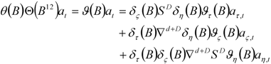
The TRAMO/SEATS package (see Gómez and Maravall [11,12], for documentation and Kaiser and Maravall [13], for a related cycle extraction procedure based on the package) is used to automatically identify an outlier-adjusted multiplicative seasonal ARIMA model for each price, now denoted generically as , of the form

(2)

The exact type and timing of each of the K interventions is automatically identified, with four types of outliers being considered: innovational outliers (IO), additive outliers (AO), level shifts (LS) and temporary changes (TC) (see Gómez and Maravall [11] for further details). In (2) denotes a white noise series of innovations with zero mean and variance . The various lag polynomials are defined as

SEATS imposes the following constraints: , , and . Writing (2) as (with for simplicity)

(3)

then, on the assumption that the components are uncorrelated, SEATS factorizes the autoregressive polynomial using the following rule. If denotes the frequency of a root of expressed in radians, then if the root is allocated to the trend-cycle ; if , , the root is allocated to the seasonal, ; and if takes any other value then it is allocated to the irregular component, . Hence cycles with a period longer than a year will be part of the trend-cycle, while cycles with a period less than a year will go into the irregular. This rule allows the autoregressive polynomial to be factorized as and (3) to be rewritten

in which is the annual aggregation operator, so that . The components will thus have models of the form

(4a)

(4b)

(4c)

with , and being mutually uncorrelated. Consistency between the “reduced form” (3) and the “structural model” (4) requires the moving average polynomials in the structural model to satisfy the identity

The Weiner-Kolmogorov (WK) estimator of the trend-cycle component is then given by (see, for example, Kaiser and Maravall [13])

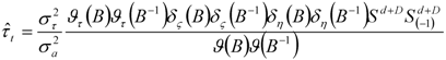
where the notation is employed. SEATS provides algorithms for obtaining this estimator in finite samples, where backcasts and forecasts calculated from the reduced form (3) are used to extend the observed series to allow the WK estimator to be computed (and, indeed, WK estimators of the other components) throughout the entire sample.

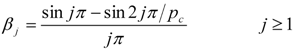
Given the trend-cycle component , the cycle can be removed to leave just the trend by using a low-pass filter, of which several alternatives are available (for example, the Hodrick-Prescott [14] and Baxter-King [15] filters). We propose using the low-pass version of the Christiano and Fitzgerald random walk (with drift adjustment) CF filter [16], which has been shown to be robust and a close to optimal filter for a wide range of time series. The form that the filter takes here is

where is the asymmetric high-pass filter that passes all components with periods of oscillation less than (this filter provides an optimal linear approximation to when the data follows a random walk and extremely good performance when the data are more generally non-stationary). For the “CF filter” is

(See Christiano and Fitzgerald [16] for adaptations of this formula for the end-points and ). The CF filter thus “takes out” of the trend-cycle all components having cycles with periods less than .

Having thus obtained the estimated trend components for each price, they may then be combined using (1) and an appropriate set of weights to obtain an estimated core inflation series.

3. Core Inflation Estimates for the U.K.

The example used to illustrate this technique is based on the current U.K. retail price index (RPI) section structure, which contains 14 sections whose indices are available monthly from 1987 (see ONS [17]). We emphasise that this example is merely illustrative, not least because it is CPI inflation that is now targeted in the U.K. However, the example is sufficiently rich to enable a detailed application of the technique to be undertaken, reported and interpreted.

The logarithms of the section indices, along with the logarithm of the RPI itself, are plotted for the period up to December 2011 in Figure 1 and show a wide range of non-stationary behaviour, having disparate trends, seasonal patterns and volatility.

The reduced form and trend-cycle component models selected by TRAMO/SEATS for each of the sections are reported in Table 1 (note that the outliers are automatically identified and accounted for in the model fitting). All trend-cycles are non-stationary so that the CF filter should provide an excellent approximation to the underlying trend component.

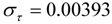
Figure 2 shows trend inflation, calculated as , for the six sections having the largest 2011 weights (covering approximately 70% of the RPI), along with the actual inflation rates for the sections. Two trend inflations are shown, for and 96, which pass components to the trend having periods in excess of and 8 years respectively (these represent the typical business cycle bounds used in macroeconomics: see, for example, Baxter and King [15]). The smaller setting follows actual inflation very closely, which is not surprising given that this setting only excludes components with periods between 12 and 18 months from the trend-cycle to obtain . The larger setting produces more slowly varying trends as it concentrates mainly on the long-period, low frequency components at the exclusion of higher frequency components.

Table 1. Reduced form and trend-cycle component models obtained by TRAMO/SEATS.

Section	Reduced form	Trend-cycle
Alcohol
6 outliers (1990.04 LS; 1990.05 LS; 1991.04 LS; 2008.04 LS; 2011.01 LS; 2011.04 LS)
Catering
4 outliers (1991.04 LS; 2008.12 LS; 2010.01 LS; 2011.1 LS)
Cigarettes & tobacco
5 outliers (1989.04 LS; 1991.04 LS; 1999.09 LS; 2000.04 LS; 2011.04 LS)
Clothing & footwear
6 outliers (2000.07 LS; 2008.12 LS; 2010.02 LS; 2010.04 LS; 2010.09 LS; 2011.02 LS)
Fares
6 outliers (1990.01 AO; 2003.04 TC; 2003.12 AO; 2004.12 AO; 2006.05 LS; 2011.04 AO)
Food
1 outlier (2008.06 LS)
Fuel & light
5 outliers (1990.10 AO; 2008.02 LS; 2008.09 TC; 2010.02 LS; 2010.12 AO)
Household goods
6 outliers (1991.04 LS; 2006.12 AO; 2007.03 AO; 2007.06 LS; 2007.07 LS; 2008.06 AO)
Household services
3 outliers (1991.04 LS; 1995.07 LS; 2006.10 TC)
Housing
6 outliers (1988.08 LS; 1990.04 LS; 1991.04 LS; 1993.01 AO; 1993.04 TC; 2008.12 LS)
Leisure goods
6 outliers (1991.03 AO; 2006.02 TC; 2007.06 TC; 2008.12 TC; 2010.01 AO; 2011.06 LS)
Leisure services
6 outliers (1987.09 AO; 1988.04 LS; 1991.04 LS; 1991.09 TC; 1992.04 LS; 1992.09 TC; 2002.04 LS)
Motoring
1 outlier (2008.11 LS)
Personal goods & services
5 outliers (1994.02 AO; 1994.05 AO; 1994.08 TC; 1994.12 AO;; 1998.02 LS)

Table 1. Reduced form and trend-cycle component models obtained by TRAMO/SEATS.

Section	Reduced form	Trend-cycle
Alcohol
6 outliers (1990.04 LS; 1990.05 LS; 1991.04 LS; 2008.04 LS; 2011.01 LS; 2011.04 LS)
Catering
4 outliers (1991.04 LS; 2008.12 LS; 2010.01 LS; 2011.1 LS)
Cigarettes & tobacco
5 outliers (1989.04 LS; 1991.04 LS; 1999.09 LS; 2000.04 LS; 2011.04 LS)
Clothing & footwear
6 outliers (2000.07 LS; 2008.12 LS; 2010.02 LS; 2010.04 LS; 2010.09 LS; 2011.02 LS)
Fares
6 outliers (1990.01 AO; 2003.04 TC; 2003.12 AO; 2004.12 AO; 2006.05 LS; 2011.04 AO)
Food
1 outlier (2008.06 LS)
Fuel & light
5 outliers (1990.10 AO; 2008.02 LS; 2008.09 TC; 2010.02 LS; 2010.12 AO)
Household goods
6 outliers (1991.04 LS; 2006.12 AO; 2007.03 AO; 2007.06 LS; 2007.07 LS; 2008.06 AO)
Household services
3 outliers (1991.04 LS; 1995.07 LS; 2006.10 TC)
Housing
6 outliers (1988.08 LS; 1990.04 LS; 1991.04 LS; 1993.01 AO; 1993.04 TC; 2008.12 LS)
Leisure goods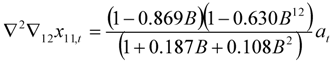
6 outliers (1991.03 AO; 2006.02 TC; 2007.06 TC; 2008.12 TC; 2010.01 AO; 2011.06 LS)
Leisure services
6 outliers (1987.09 AO; 1988.04 LS; 1991.04 LS; 1991.09 TC; 1992.04 LS; 1992.09 TC; 2002.04 LS)
Motoring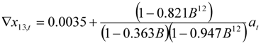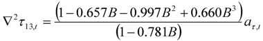
1 outlier (2008.11 LS)
Personal goods & services
5 outliers (1994.02 AO; 1994.05 AO; 1994.08 TC; 1994.12 AO;; 1998.02 LS)

Figure 1. Logarithms of the RPI and its sections, 1987-2011 (2011 section weights shown in parentheses).

Figure 1. Logarithms of the RPI and its sections, 1987-2011 (2011 section weights shown in parentheses).

Figure 2. Section trend inflation.

Figure 2. Section trend inflation.

Figure 3. Section weights, 1987–2011.

Figure 3. Section weights, 1987–2011.

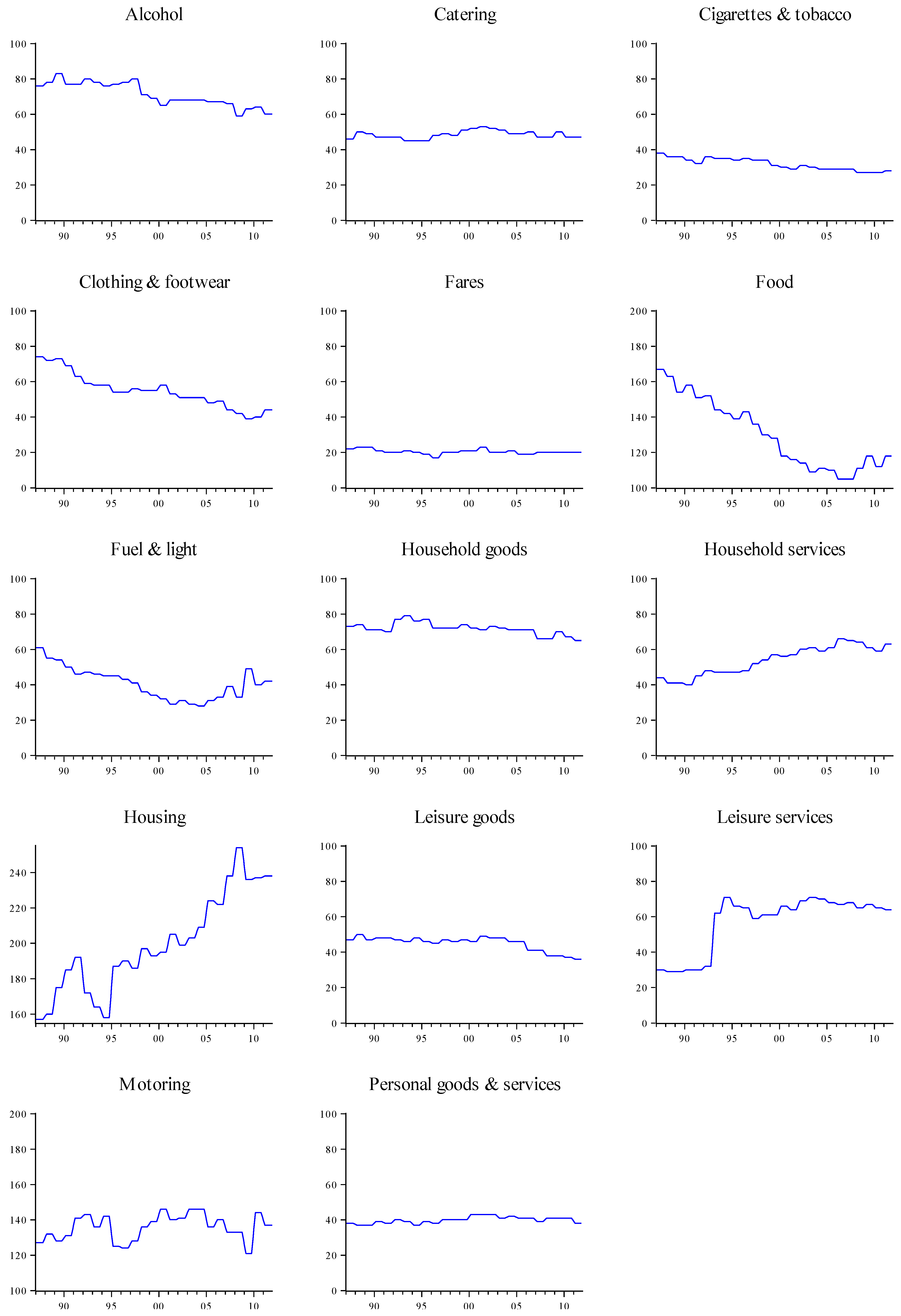
To compute core inflation requires a complete set of weights , , for the sample period 1987 to 2011. The weights are updated by the ONS every year, and Figure 3 shows these section weights (the convention is that the weights sum to 1000). These weights were then used to compute annual core inflation using (1) (the weights were smoothed by linear interpolation across the last two months of one year and the first two months of the next year to avoid the (albeit small) jumps in inflation that result from the annual weight updating).

Figure 4. Actual and core inflation, 1987–2011, with forecasts to 2013.

Figure 4. Actual and core inflation, 1987–2011, with forecasts to 2013.

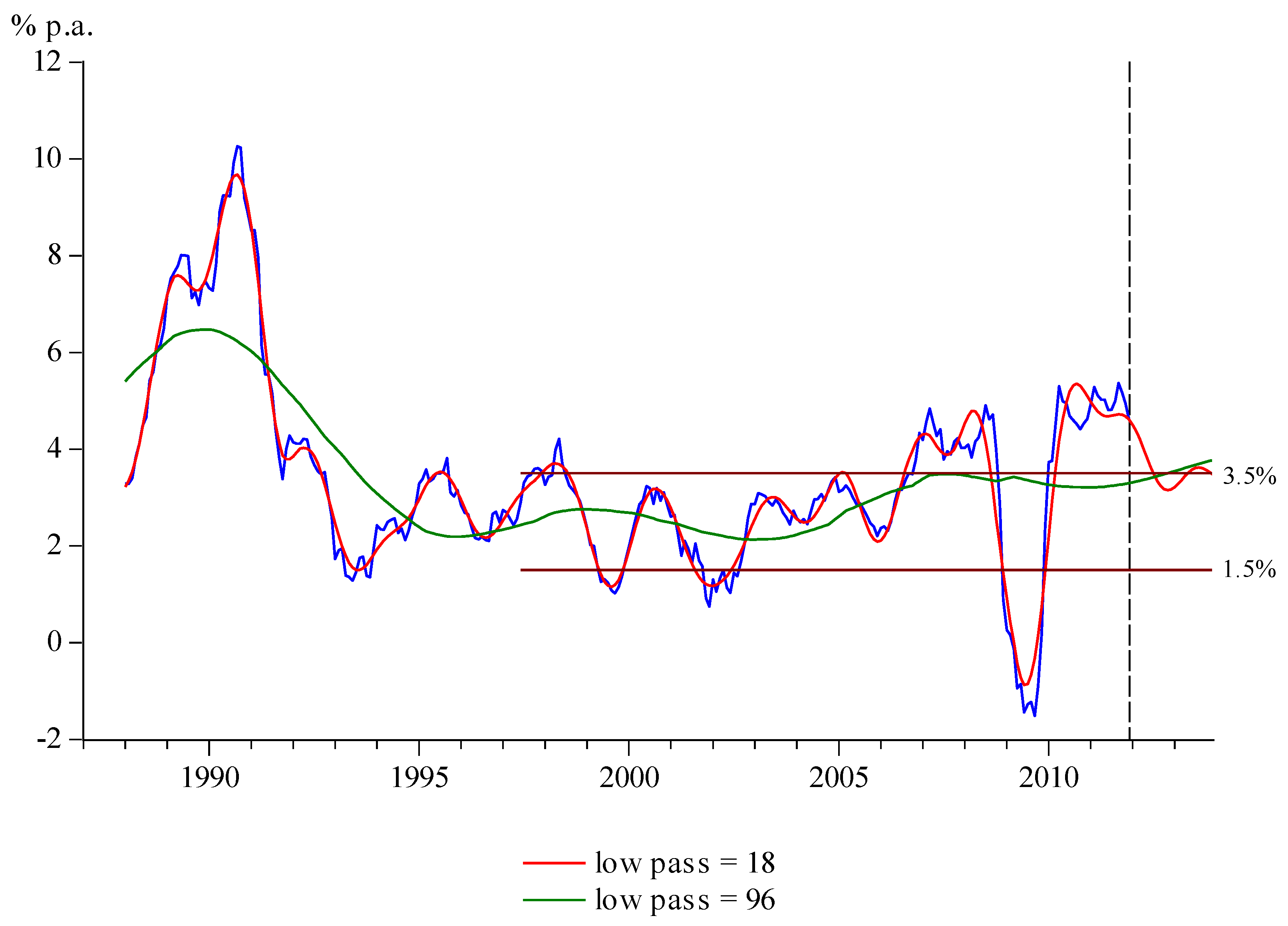
Figure 4 shows the two core inflation series obtained using and 96 along with the observed inflation series calculated as . Although this series is clearly not RPI inflation (the method of computing this in practice being much more detailed), the correlation between the two is in excess of 0.999 and plots of the two are indistinguishable from each other. With the lower setting of core inflation is essentially a smoothed version of actual inflation, but the higher setting produces a core inflation series that slowly varies through time: in fact, since the middle of 1993 it has consistently lain in the range 2 to % per annum.

The two core inflation series are actually shown in Figure 4 up to the end of 2013. The last 24 values are forecasts of future core inflation from a December 2011 origin. Their construction uses the forecasts of the trend-cycle components produced automatically by TRAMO using the models shown in Table 1. The expenditure weights used in the forecasts are held at their December 2011 values. Using forecasts of the trend-cycle components has the additional benefit of enabling the estimates of the trend components obtained from the low-pass filter to be computed with less error as the end of the sample is reached.

Figure 4 also shows the target band for RPI inflation set on Bank of England independence in 1997.2 Core inflation for the setting is seen to have historically always lain within this band but is forecast to be 3.8% by the end of 2013, having breached the band in the middle of 2013. As has been mentioned above, setting , on the other hand, leads to much wider variation in core inflation with the bands being broken regularly from 2006, although this core inflation is forecast to be just under 3.5% by the end of 2013.

4. Alternative Weighting Schemes

There have been several recent proposals for using weights other than those based on expenditure. Persistence weights, first proposed by Cutler [18] (for a more recent application, see Bilke and Stracca [19]), are based on the predictability of the section indices: those sections whose rate of inflation is more predictable are given higher weights in the core inflation calculation. 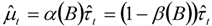If the predictability of the growth rate of the trend-cycle component is the focus of attention, then a model for the stationary transformation (the monthly change in the annual inflation rate of the trend-cycle component) is required. If the model for is of the form

(i.e., , which is the typical case from Table 1), then, on noting that , we have

or

Defining persistence as and noting that when , , then

which may be calculated directly from the models reported in Table 1. For cigarettes & tobacco and fuel & light, which contain no seasonality, the autoregressive operator is so that and . Four further sections have negative but finite persistence weights: food, household services, motoring and personal goods & services (household services and motoring have reduced form representations embodying stationary seasonality). As it is traditional in these cases to set the persistence weight to zero whenever , these six sections are thus assigned zero weights. For the two cases when (catering and leisure goods), , so that and .

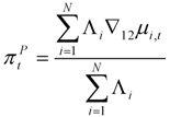
The section persistence weights, , may be used in two ways. First, they can replace the expenditure weights in (1) to produce the persistence weighted measure of core inflation (noting that in this application the weights remain constant through time)

Second, the persistence weights can be applied to the expenditure weights to obtain the “double-weighted” (using the terminology of Silver, [5]) core inflation measure

Table 2 provides the persistence weights so calculated for each section of the RPI. The persistence-weighted core inflation measures and are thus akin to F&E (food and energy) exclusion-based measures of core inflation.

Table 2. Section persistence weights.

Section	Persistence weights
Alcohol	0.094
Catering	1
Cigarettes & tobacco	0 ( )
Clothing & footwear	0.644
Fares	0.625
Food	0 (-0.812)
Fuel & light	0 ( )
Household goods	0.437
Household services	0 (–1.133)
Housing	0.536
Leisure goods	1
Leisure services	0.573
Motoring	0 (–2.042)
Personal goods & services	0 (–0.344)

Table 2. Section persistence weights.

Section	Persistence weights
Alcohol	0.094
Catering	1
Cigarettes & tobacco	0 ( )
Clothing & footwear	0.644
Fares	0.625
Food	0 (-0.812)
Fuel & light	0 ( )
Household goods	0.437
Household services	0 (–1.133)
Housing	0.536
Leisure goods	1
Leisure services	0.573
Motoring	0 (–2.042)
Personal goods & services	0 (–0.344)

Figure 5 shows the two sets of persistence weighted core inflations, again with forecasts out to end-2013 using extrapolated end-2011 expenditure weights in . These core inflations are rather more variable than those that use “simple” expenditure weights but again those using the frequency setting tend to lie within the % band from 1998 and throughout the forecast period. Whether these core inflation estimates represent improvements over those computed in Section 3 is, however, debatable. The fixed weights used in may be considered to be a drawback, which is only partially alleviated in , while the exclusion of so many sections in both measures (six in all) may be felt to be too draconian. Nevertheless, and are easily computable and might be thought to provide useful additional information on core inflation.

5. Multivariate Approaches to Constructing Core Inflation

Proietti proposes using a multivariate structural time series model to compute core inflation [20]. This structural model for the prices making up the index takes the form

where and , , and are defined analogously, the latter trio of disturbances being assumed to be mutually uncorrelated. The individual prices thus have potentially correlated stochastic trends having potentially correlated stochastic slopes. Given an appropriate vector or matrix of weights, a measure of core inflation can then be constructed using the estimated annual trend differences . This approach takes into account that individual prices might be contemporaneously correlated, but necessarily assumes that the individual prices all follow the same form of stochastic process. On examining Figure 1, this is clearly unlikely to be the case for the sections of the RPI and hence we do not investigate this model any further.

Valle e Azevedo considers multivariate band-pass filters which could be used to remove the cyclical components from the trend-cycles [21]. He shows, however, that this approach will only offer substantial improvements over the univariate case considered in this paper if the individual prices are highly correlated, which does not seem to be the case here (the maximum absolute correlation between the monthly changes of the sections is 0.7 and most correlations are much smaller than this).

6. Discussion and Conclusions

Measures of core inflation will continue to be a useful input into economic policy making and it is argued here that the approach proposed in this paper has several advantages. First, it is constructed using the trend components of the individual prices extracted from detailed modelling of their stochastic structure. Second, it is straightforward to compute several measures of core inflation based on these trend components, including their forecasts. All computations were performed in EVIEWS (EViews [22]), which is perhaps the “industry standard” for time series econometrics, and thus these measures do not require specialized software (TRAMO/SEATS is one of the seasonal adjustment procedures available in EVIEWS). Since the process can be fully automated, models for individual prices may be updated each month so that current developments can be incorporated as swiftly as possible.

Figure 5. Weighted core inflation: top panel ; bottom panel .

Figure 5. Weighted core inflation: top panel ; bottom panel .

Although this approach to constructing a core inflation measure has used the section structure of the U.K. RPI for illustration, it should be clear that the methodology can be used on any set of individual prices for which an overall measure of core inflation is required: the U.K. CPI would be a prime candidate. The setting of the cut-off value p_c may also be varied by the user: for example, choosing p_c = 37 would be consistent with some earlier proposals (see Mankikar and Paisley [3], Appendix A) which thought that this would be a suitably long time horizon over which relative prices would have adjusted to shocks. The forecast horizon may also be chosen to be other than 24 months: for example, Bank of England inflation projections are for up to three years ahead. We would therefore recommend this approach for serious consideration if automatic computation and updating of core inflation measures is required.

References and Notes

- R.J. Gordon. “The impact of aggregate demand on prices.” Brookings Papers on Econ. Activ. 3 (1975): 613–670. [Google Scholar] [CrossRef]
- O. Eckstein. Core Inflation. Englewood Cliffs, NJ, USA: Prentice Hall, 1981. [Google Scholar]
- A. Mankikar, and J. Paisley. Core Inflation: A Critical Guide. working paper No. 242; London, UK: Bank of England, 2004. [Google Scholar]
- R. Rich, and C. Steindel. “A comparison of measures of core inflation.” Econ Pol Rev Dec 13 (2007): 19–38. [Google Scholar]
- M. Silver. Core Inflation: Measurement and Statistical Issues in Choosing Among Alternative Measures. IMF Staff papers 54; Washington, DC, USA: International Monetary Fund, 2007, pp. 163–190. [Google Scholar]
- M.A. Wynne. Core Inflation: A Review of Some Conceptual Issues. Federal Reserve Bank of St Louis Review 90; St. Louis, MO, USA: Federal Reserve Bank of St Louis, 2008, pp. 205–228. [Google Scholar]
- D. Quah, and S.P. Vahey. “Measuring core inflation.” Econ. J. 105 (1995): 1130–1144. [Google Scholar] [CrossRef]
- M. Pedersen. “An alternative core inflation measure.” Ger. Econ. Rev. 10 (2009): 139–164. [Google Scholar] [CrossRef]
- A.S. Blinder. Federal Reserve Bank of St Louis Review 79. Federal Reserve Bank of St Louis Review 79; St. Louis, MO, USA: Federal Reserve Bank of St Louis, 1997, pp. 157–160. [Google Scholar]
- T. Cogley. “A simple adaptive measure of core inflation.” J. Money Credit Bank. 34 (2002): 94–113. [Google Scholar] [CrossRef]
- V. Gómez, and A. Maravall. Program SEATS “Signal Extraction in ARIMA Time Series” Instructions for the User. EUI working paper ECO no. 94/28; San Domenico di Fiesole, Italy: European University Institute, 1994. [Google Scholar]
- V. Gómez, and A. Maravall. Program TRAMO “Time Series Regression With ARIMA Noise, Missing Observations, and Outliers” Instructions for the User. EUI working paper ECO no. 94/31; San Domenico di Fiesole, Italy: European University Institute, 1994. [Google Scholar]
- R. Kaiser, and A. Maravall. “Combining filter design with model-based filtering (with an application to business-cycle estimation).” Int. J. Forecasting 21 (2005): 691–710. [Google Scholar] [CrossRef]
- R.J. Hodrick, and E.C. Prescott. “Postwar U.S. business cycles: An empirical investigation.” J. Money Credit Bank. 29 (1997): 1–16. [Google Scholar] [CrossRef]
- M. Baxter, and R.G. King. “Measuring business cycles: Approximate band-pass filters for economic time series.” Rev. Econ. Stat. 81 (1999): 575–593. [Google Scholar] [CrossRef]
- L.J. Christiano, and T.J. Fitzgerald. “The band pass filter.” Int. Econ. Rev. 44 (2003): 435–465. [Google Scholar] [CrossRef]
- Office for National Statistics (ONS), Consumer Price Indices Technical Manual, 2010 Edition. Newport, UK: Office for National Statistics, 2010.
- J. Cutler. A New Measure of Core Inflation in the U.K. MPC unit discussion paper No. 3; London, UK: Bank of England, 2001. [Google Scholar]
- L. Bilke, and L. Stracca. “A persistence-weighted measure of core inflation in the Euro area.” Econ. Model. 24 (2007): 1032–1047. [Google Scholar] [CrossRef]
- T. Proietti. “Measuring core inflation by multivariate structural time series models.” In Advances in Computational Economics, Finance and Management Science: Optimisation, Econometric and Financial Analysis. Edited by E.J. Kontoghiorghas and C. Gatu. Berlin, Germany: Springer, 2007, pp. 205–223. [Google Scholar]
- J. Valle e Azevado. “A multivariate band-pass filter for economic time series.” J. R. Stat. Soc. Ser. C Appl. Stat. 60 (2011): 1–30. [Google Scholar] [CrossRef]
- “EViews.” In EViews User Guide Version 7. Irvine, CA, USA: Quantitative Micro Software, 2009.
- 1These letters may be found at http://www.bankofengland.co.uk/monetarypolicy/inflation.htm
- 2The target was actually set for the RPIX (RPI excluding mortgage interest repayments) but we use the bounds here as a convenient reference point.
© 2013 by the authors; licensee MDPI, Basel, Switzerland. This article is an open access article distributed under the terms and conditions of the Creative Commons Attribution license (http://creativecommons.org/licenses/by/3.0/).
Share and Cite
Mills, T.C. Constructing U.K. Core Inflation. Econometrics 2013, 1, 32-52. https://doi.org/10.3390/econometrics1010032
Mills TC. Constructing U.K. Core Inflation. Econometrics. 2013; 1(1):32-52. https://doi.org/10.3390/econometrics1010032
Chicago/Turabian StyleMills, Terence C. 2013. "Constructing U.K. Core Inflation" Econometrics 1, no. 1: 32-52. https://doi.org/10.3390/econometrics1010032
APA StyleMills, T. C. (2013). Constructing U.K. Core Inflation. Econometrics, 1(1), 32-52. https://doi.org/10.3390/econometrics1010032