A Calibration Report for Wireless Sensor-Based Weatherboards

Abstract

Sub-Saharan Africa contains the highest number of people affected by droughts. Although this can easily be mitigated through the provision of timely, reliable and relevant weather forecasts, the sparse network of weather stations in most of these countries makes this difficult. Rapid development in wireless sensor networks has resulted in weatherboards capable of capturing weather parameters at the micro-level. Although these weatherboards offer a viable solution to Africa’s drought, the acceptability of such data by meteorologists is only possible if these sensors are calibrated and their field readiness scientifically evaluated. This is the contribution of this paper; we present results of a calibration exercise that was carried out to: (1) measure and correct lag, random and systematic errors; (2) determine if Perspex was an ideal material for building sensor boards’ enclosures; and (3) identify sensor boards’ battery charging and depletion rates. The result is a calibration report detailing actual error and uncertainty values for atmospheric pressure, humidity and temperature sensors, as well as the recharge and discharge curves of the batteries. The results further ruled out the use of Perspex for enclosing the sensor boards. These experiments pave the way for the design and implementation of a sensor-based weather monitoring system (SenseWeather) that was piloted in two regions in Kenya.

1. Introduction

According to the World Disasters Report of 2013, Africa contained 56% of the droughts that occurred between 2003 and 2012; they affected 26% of her population. Most of these occurred in Sub-Saharan Africa (SSA) [1]. The uniqueness of the problem in SSA is the inadequacy and ineffectiveness of the region’s preparedness for these disasters [2,3]. This is partly attributed to the fact that the meteorological institutions (the National Meteorological Services (NMSs)) charged with weather forecasting rely on weather stations that are thousands of kilometers apart [4,5].

The now readily-available, versatile and less expensive wireless sensor network (WSN)-based weather stations (or weather sensor boards) could be used to address this problem; they can enable capturing of weather parameters at the micro-level, hence downscaling the forecasts. In [6], an integrated drought early warning system, ITIKI (Information Technology and Indigenous Knowledge with Intelligence), that delivers a drought early warning system (DEWS) composed of three elements: (1) drought knowledge (2) drought monitoring and prediction; and (3) drought communication and dissemination. In this (ITIKI) project, weatherboards by Libelium [7] were used to collect real-time weather data. The drought knowledge component entailed the systematic collection of data on droughts and assessment of drought risk; it was built from two sources: indigenous knowledge and structured weather data from sensor-based weather meters and conventional weather stations. The sensor-based weather meters were first calibrated before being used in the project (ITIKI); this is the sensor calibration exercise described in this paper.

For the sensor readings to be acceptable by the meteorologists, there must be scientifically proven assurance that these readings are the same as those from professional weather stations calibrated and certified by World Meteorological Organization (WMO). The term calibration is defined in [8] as “the set of operations which establish, under specified conditions, the relationship between values indicated by a measuring instrument or measuring system, or values represented by a material measure, and the corresponding known values of a measurand (the physical quantity being measured)”. Sensor calibration is the first step towards achieving this, and it involves comparing the readings from the sensors against accepted standards to determine how closely the sensors’ output matches the set standards over the expected range of operation. Such calibration is achieved by following a set of WMO-stipulated calibration tasks upon whose completion, a calibration report/certificate is produced.

Motivated by the need to provide timely, accessible and reliable/acceptable/effective/relevant weather forecasts to improve agriculture, support operations of insurance companies and to provide credible research data to scientists, this paper revisits the issue of field readiness for sensor network by reporting on calibration work that was done in Kenya. This entailed comparing off-the-shelf agriculture sensor boards with professional weather stations run by the Kenya Meteorological Department (KMD). A network of weather sensor boards was set up in the vicinity of calibrated weather stations in Nairobi/Kenya, and readings were taken in parallel from both the sensors and the weather stations on a 24 h a day, seven days a week basis for a period of one year. The results obtained, using the absolute mean percentage error (MAPE) and root mean square error (RMSE) as comparative metrics, revealed that the sensor readings had impressive accuracies, ranging from 92% to 99%. Given the many other advantages associated with the use of weather sensor boards, we went ahead to embark on using the calibrated sensors to implement sensor-based weather monitoring in Kenya.

The first objective of this exercise was to investigate the suitability and field readiness of selected weatherboards in weather monitoring. This objective was meant to answer the following questions:

(a)

What is the accuracy of the sensors?

(b)

What is the variability of measurements in a network containing such sensors?

(c)

What change, or bias, will there be in the data provided by the sensor if its siting location is changed?

(d)

What change or bias will there be in the data if it replaces a different sensor measuring the same weather element(s)?

This was achieved by assessing the following factors:

(1)

The sensors boards’ lag errors; these result from: delay statements used for stabilizing power supply after waking up the sensor boards; the process of storing the readings in secure digital (SD) cards; print and println statements; and general packet radio service (GPRS) commands;

(2)

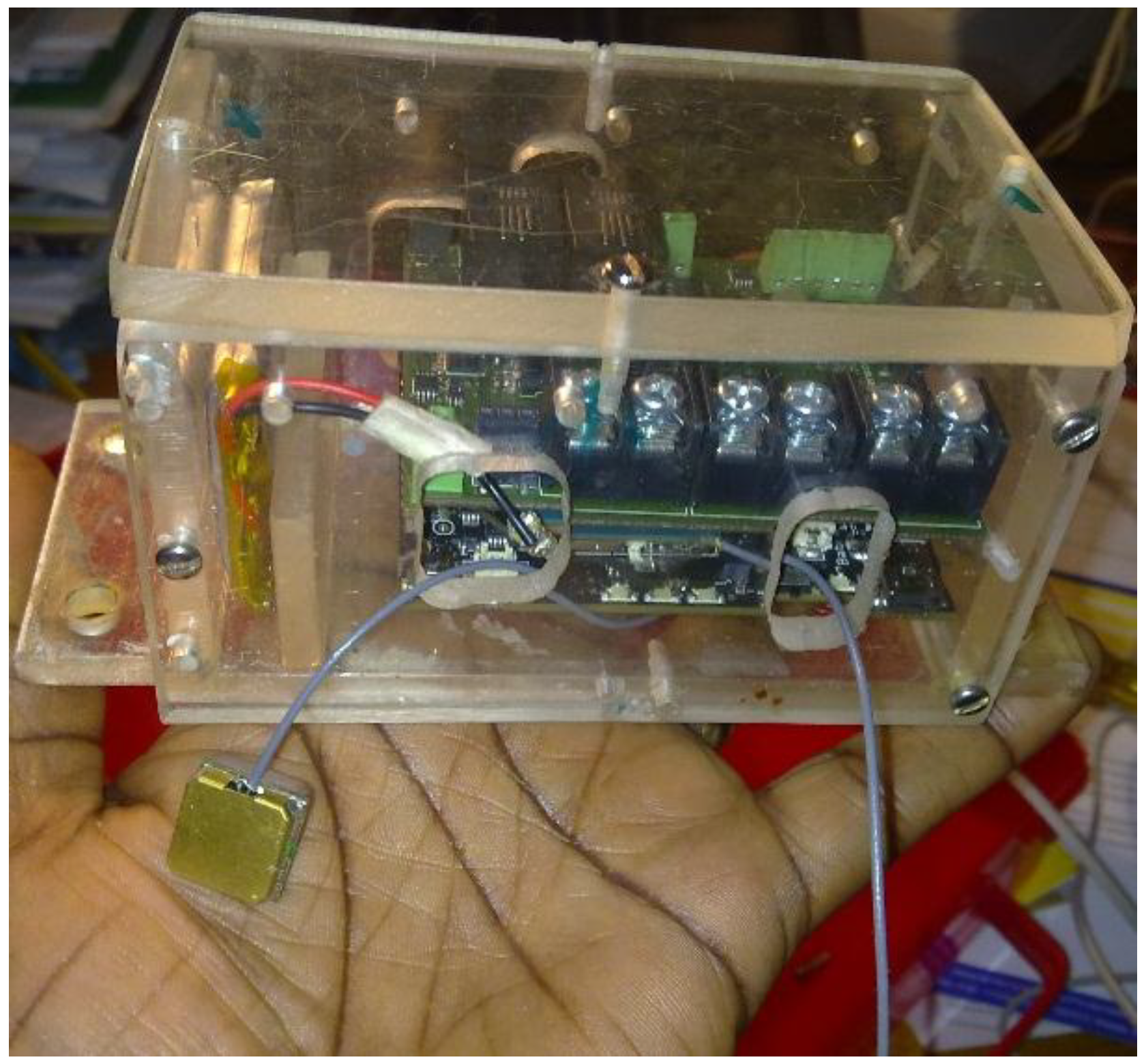
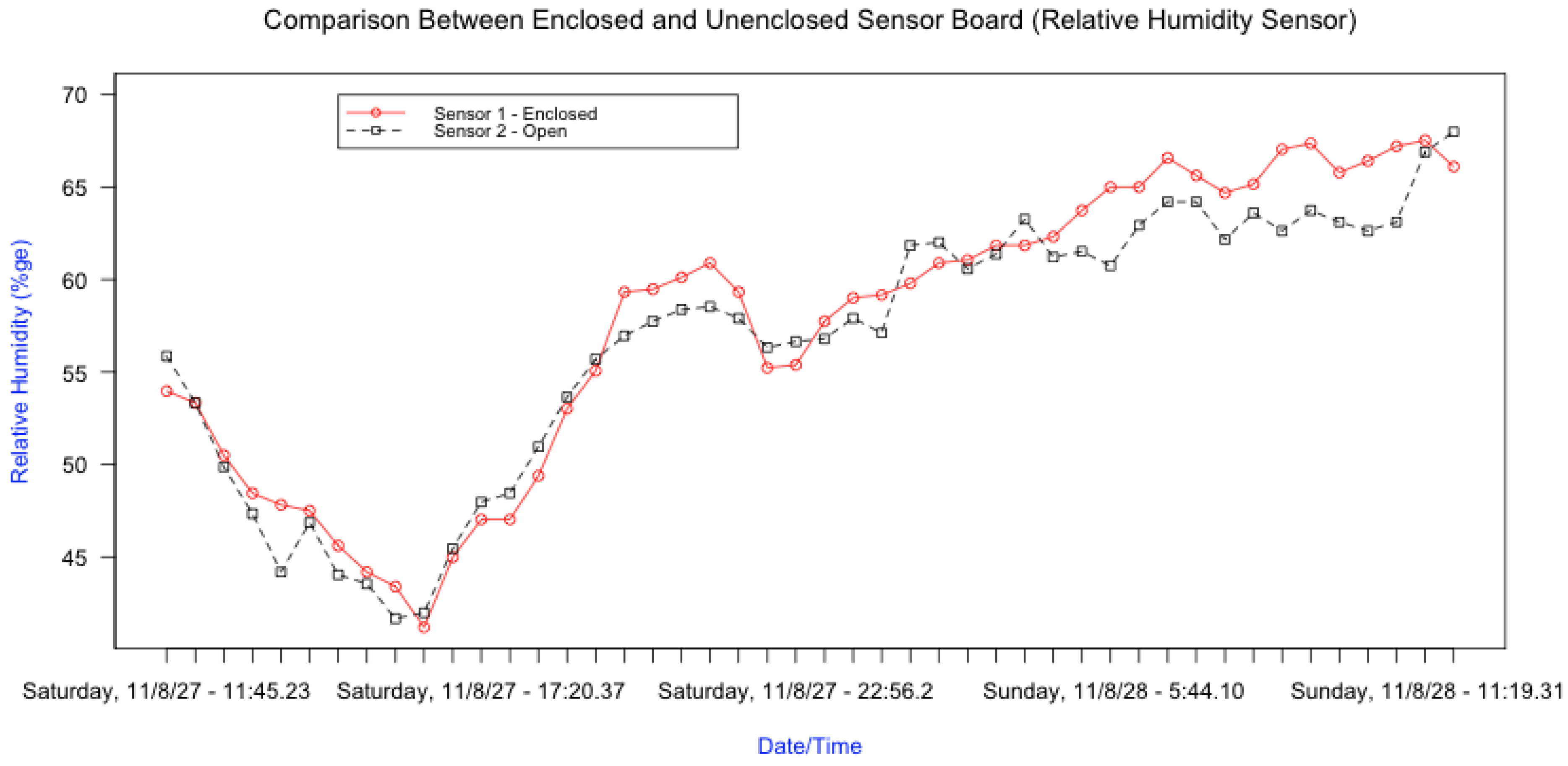
The effects of enclosing the sensor boards in a Perspex enclosure;

(3)

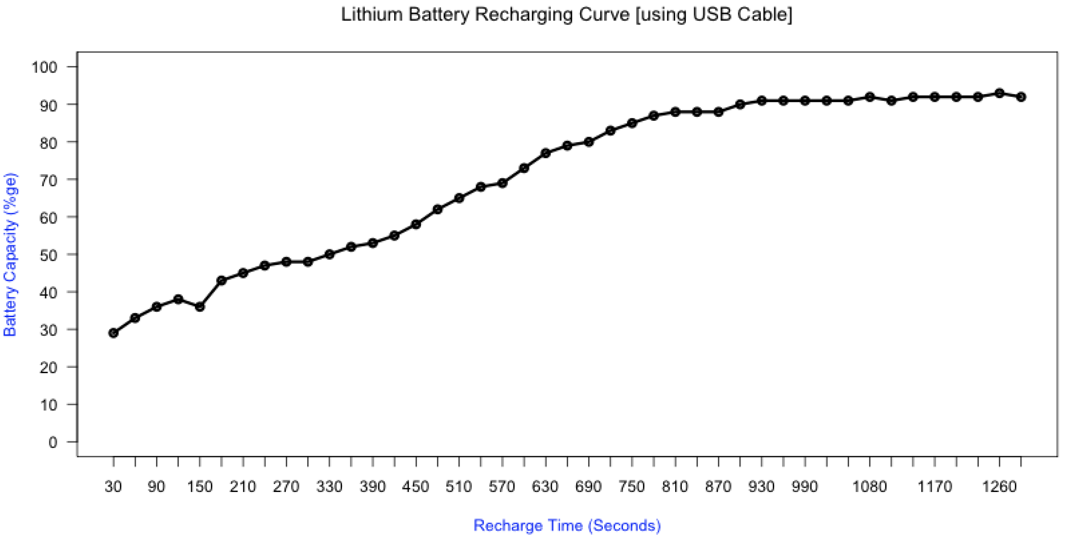
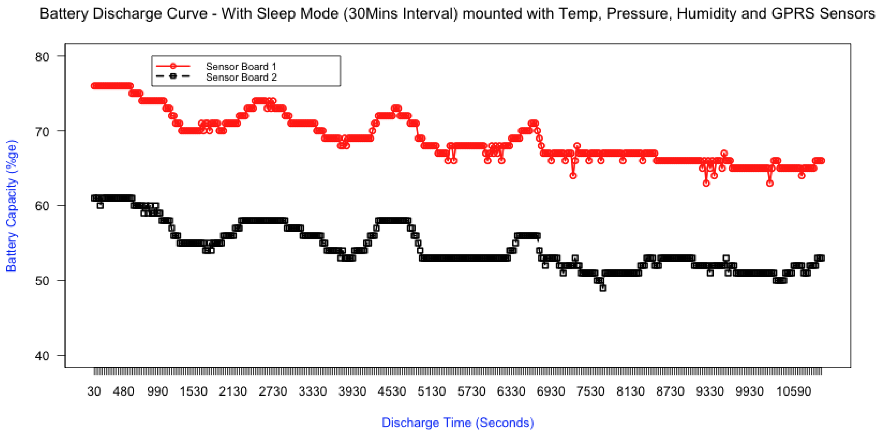
The sensors boards’ battery discharge and recharge curves; this would enable one to know the frequency with which the deployed sensors’ batteries needed to be recharged/replaced.

Further, calibration exercises between the sensor boards and professional weather stations were carried out. This qualitatively and quantitatively gave the measures of the readiness (for field deployment) of weather sensor boards in terms of:

(1)

The reliability and stability of the sensors;

(2)

The convenience of the operation and maintenance of the sensors boards;

(3)

The sensors’ durability; and

(4)

The acceptability of the sensors in terms of their initial cost, as well as the cost of their consumables and spare parts.

The second objective was to use the results of the calibration exercise to design, implement and evaluate a sensor-based weather monitoring system (SenseWeather) for two selected regions in Kenya. The resulting generic system is a complementary solution to the networks of professional weather stations run by meteorological institutions in SSA. It also acts as a tool that can be used by small-scale farmers and insurers to mitigate the effects of droughts and other weather-related disasters.

The remainder of this paper is structured as follows. Section 2 describes related literature, while Section 3 details the experimental setup. Section 4 describes the results, and finally, the conclusion and further work are contained in Section 5.

2. Background Literature

2.1. About the Kenya Meteorological Department

The weather instruments operated at the Observatory Unit of the Kenya Meteorological Department (KMD) were used for the calibration experiments described in this paper. KMD (formerly the East African Meteorological Department (EAMD)) is a department (under a ministry) of the Government of Kenya and was established in 1977 [5]. KMD is both a national (Kenya) and regional (the Horn of Africa) center for drought forecasting and other related activities, and as such, the Department is equipped with an array of weather monitoring equipment. The Observatory Unit, which is responsible for making weather observations of every kind, for instance, manning a manual weather station that is operated 24 h a day, seven days week. The Unit also has an automatic weather station (AWS) from which weather parameters are automatically relayed to their computer systems.

2.2. Weather Instruments Calibration Guidelines

In the Guidelines on Climate Observation Networks and Systems [8], the requirements for the weather equipment’s resolution and accuracy are stipulated. Here, the steps of calibrating sensor equipment are listed as follows: (1) reviewing the sensors’ performance against the manufacturer’s specifications; (2) laboratory tests against a reference identical standard; this is to determine their accuracies and robustness (for example, a relative humidity sensor should be compared against a weather instrument for measuring relative humidity); and (3) field-tests in the operational environment; this should be done in parallel with the reference standard and preferably on multiple sites. Further, in order to test the sensors’ behavior across the expected range of climatic conditions, the field tests should run for at least one year.

Calibration enforces the requirement that standards are maintained across the globe; hence, ensuring uniformity in publication and interpretation of weather observations and the statistics therein. As such, calibration is part of the quality assurance program of the World Meteorological Organization (WMO). Other components of this program are instrument testing, a clear definition of the requirements, instrument selection, siting criteria, maintenance and logistics.

The output of a calibration exercise is documented in a calibration report or calibration certificate, and it should spell out things, such as sensor bias (and how it can be removed either mechanically, electronically or using software), random error, application range, any existing threshold, resolution and hysteresis. Calibration must therefore be based on a particular standard, which can either be primary, secondary, international or national standards, as described in [9,10]. Other standards that could be used as a reference are working, transfer and travelling standards. Of key importance is the ability of a calibration process to be “traceable”, which is defined as “The property of the result of a measurement or the value of a standard whereby it can be related to stated references, usually national or international standards, through an unbroken chain of comparisons all having stated uncertainties.” [11].

The sensor calibration exercise described in this paper was aimed at establishing the uncertainty of the sensors, as well as other sensor characteristics related to various forms of delays. This was necessitated by the fact that the general concept of wireless sensor networks for weather monitoring is relatively new around the world and specifically in Kenya and other countries in SSA.

2.3. Calibrating for Uncertainty of Meteorological Measurements

From the perspective of sensor calibration, an error in a sensor reading is the sensor reading minus the equivalent (say temperature) reading from a reference weather station instrument. The closeness of these two values defines the accuracy of the sensor. On the other hand, the uncertainty of a sensor is the numeral expression of its accuracy; for example, a humidity sensor with an accuracy of ±1.5% has an uncertainty of 1.5. During the calibration exercises, two types of errors may reveal themselves: systematic and random errors. Random error represents stochastic fluctuations in measurement values when the measurement is repeated under identical conditions. “Systematic error is used to cover all those errors which cannot be regarded as fortuitous, as partaking of the nature of chance. They are characteristics of the system involved in the work; they may arise from errors in theory or in standards, from imperfections in apparatus or the observer, from false assumptions, etc.” [10].

In [12], one of the methods used to report the accuracy of calibration results is the “estimated systematic error and uncertainty”, where the reported estimated systematic error is later used to provide a correction value used in subsequent measurements. This is the approach that was favored in the current research, because the aim was to calculate the correction factor to be applied on the sensors before deploying them as weather stations. Once the uncertainty value for a given sensor is established through calibration, the true value can be computed as follows:

<true value> = <measured valued> ± <uncertainty>

The true value is then used to carry out other calibration conditions such as: repeatability, how close the results of successful readings are (under the same conditions) from the sensors; and reproducibility, same as repeatability, but under different conditions.

3. Experimental Section

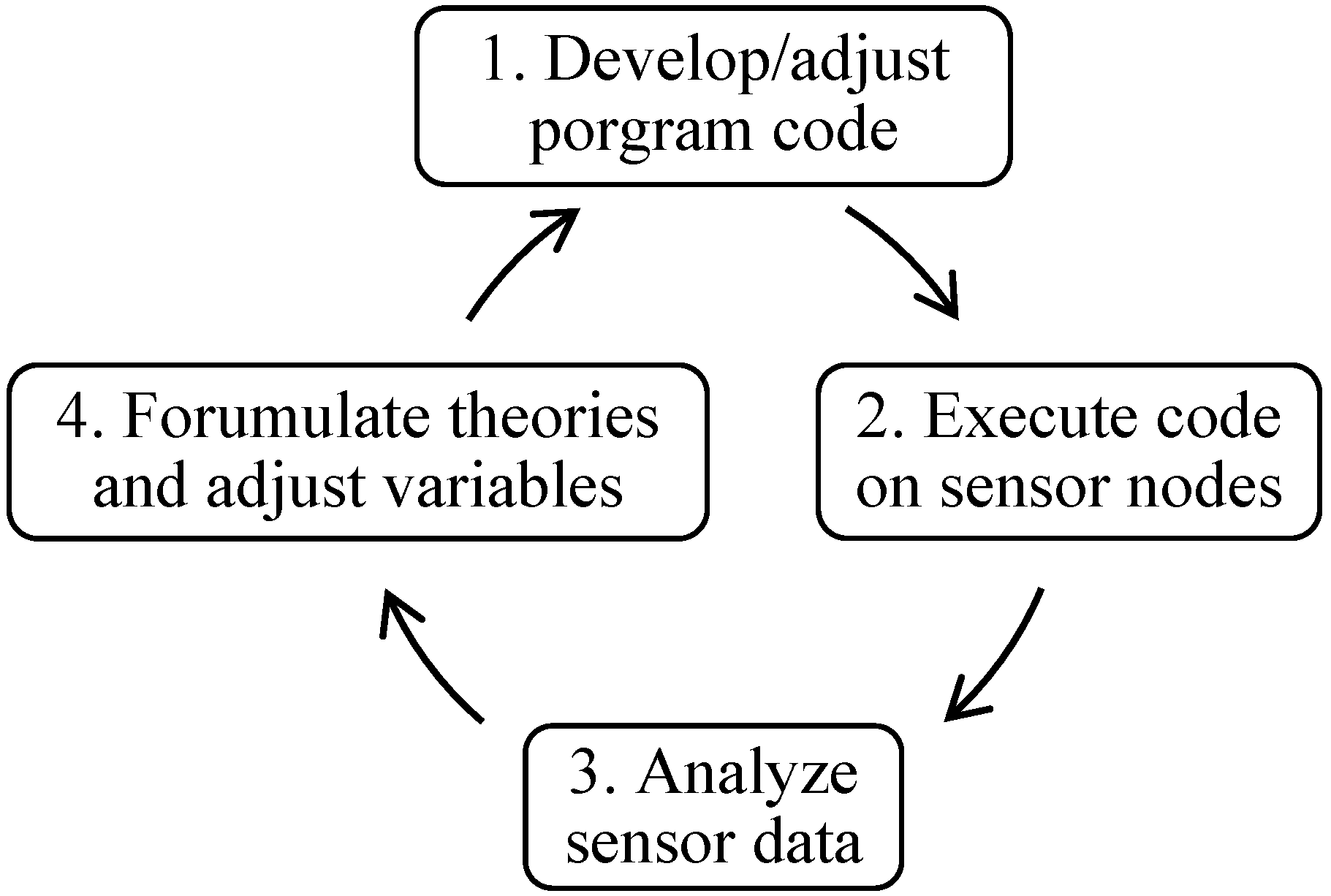
3.1. Pilot, Exploratory and Confirmatory Experiments

As per the PiECEs (Pilot, Exploratory and Confirmatory Experiments) model described in [13], the calibration experiments followed a 3-step experimental process with three types of experiments, namely pilot experiments, explanatory experiments and confirmatory experiments. This was to ensure both repeatability and reproducibility.

3.1.1. Pilot Experiments

These are small, usually short-term, experiments, which are used to test the logistics of a proposed study with the aim of gaining preliminary information. Before leaving the sensor nodes in the field for long periods of time, pilot experiments were first carried out in order to have an idea of how the various components behaved.

3.1.2. Exploratory Experiments

These are used to study the patterns of response to some parameter variations or intervention, without necessarily being based on a formal hypothesis, and may be used to generate hypotheses for more formal testing in confirmatory experiments. Wireless sensors are a relatively new technology, especially for weather monitoring in Africa. The exploratory experimentation approach was selected in order to allow for testing not just the hypothesis, but also determining whether the various components of the sensor nodes were working properly in different conditions. For instance: (1) the GSM/GPRS module may be affected by the strength of the GSM network signal; and (2) the response time of a sensor node may depend on the size of the file (on the SD card) on which the storage of the readings is taking place.

Having confirmed that sensors gave readings that correlated with those from the reference weather station, a series of four exploratory experiments were carried out to verify different aspects of the sensors’ behavior, as described below.

Exploratory Phase I: These experiments were carried out (at the Weather Observatory Unit run by the Department of Meteorology, University of Nairobi, Chiromo Campus) for a period of two weeks, and the aim was to collect adequate dataset for computing MAPE and RMSE. This resulted in MAPE values of below 5% and RMSE values less than 1.2 for all the sensors.

Exploratory Phase II: To further increase the data sample size, a second set of exploratory experiments were run at the KMD Headquarters, where unlike the Chiromo station, readings are taken twenty four hours a day, seven days a week. The MAPE and RMSE values attained matched those in Exploratory Phase I. The sensor readings were also found to be consistent (correlation coefficient of over 0.9) with those from the weather station.

Exploratory Phase III: In preparing the sensors for the real world, sensor enclosures were designed and built. After consultations with the meteorologists, Perspex material was recommended. Further, this experiment set out to find out the relationship between the board temperature (taken using the function RTC.getTemperature) and the value from the temperature sensor. The outcome here was that enclosures made from Perspex material affected the operation of the sensors; the idea of using a mini-Stephenson screen is being pursued in the future improvements of this research. On the issue of board temperature, a correlation between this reading and the one from the temperature sensor was noticed; the latter tends to be less than the prior one by 1.5 to 1.7 °C. This knowledge was incorporated into the program code running in the sensors to detect when the temperature sensors gave erroneous readings (greatly above or below the board temperature reading).

Exploratory Phase IV: After eight months of experiments, the basic procedures of using the sensors had been finalized. These included how often to charge/change batteries, where/how to place the sensors, how often the readings were observed and sent to the SMS gateway, the system prototype to receive the readings, and so on. With all of this in place, sensors were left in the field for a period of four weeks. This dataset was used to make various calibration decisions and adjustments explained in Section 4.

With all of these angles and twists to the experiment, the exploratory experimentation method was deemed best. The method has been found effective for testing instruments, which allows the simultaneous measuring of many features of an experimental system.

The entire process involved: (1) the design programs (code); (2) execution of the code on the sensor nodes; (3) statistical data analysis in both MS Excel and R; and (4) formulation and testing of theories and using them to adjust various variables.

Several cycles of the above steps were carried out as shown below (Figure 1).

Figure 1. Exploratory experiment cycles.

Figure 1. Exploratory experiment cycles.

3.1.3. Confirmatory Experiments

After the numerous cycles were carried out in the exploratory experiments phase, a number of decisions and adjustments were made at the sensor node software and hardware levels, for example: hardware level, putting the sensor nodes in an enclosed casing was ruled out; and software level, sleeping time for a sensor with GPRS module was put at 00:00:29:40 instead of 00:00:30:00.

In order to verify that the adjustments and decisions reached during the exploratory experiments were indeed correct, a series of confirmatory experiments were carried out for each adjustment/decision. These were used to test clearly-stated hypotheses, which were stated before starting the experiment. Most of these were carried out at the same time as the exploratory experiments, except for the ones involving comparing the sensor readings with the professional weather station readings.

3.1.4. Systematic Error Analysis

Further, systematic error analysis based on three error types—mean absolute percentage error (MAPE), mean error (ME) and root mean square error (RMSE)—was also applied. Inherent (to the sensor boards) errors related to various forms of delays were also analyzed. Correlation coefficients and plots, such as side-by-side boxplots, were used to run similarity tests between various datasets.

Systematic error analysis, intended to estimate the error rate between the readings from the sensor nodes and those from the professional weather station, was also carried out. Datasets consisting of hourly readings (temperature, humidity and pressure) from sensor nodes, on the one hand, and readings from the weather station, on the other, were plotted against time (for example, 0 GMT, 2 GMT…23 GMT). Taking the weather station readings as the reference, MAPE, ME and RMSE error analysis was carried out. Together with this, correlation coefficients were calculated in order to determine the (if any) linear relationship between the sensor and weather station readings.

3.2. Sensor Boards’ Inherent Errors

3.2.1. Sensor vs. Board Temperature Differences

Like many other sensor boards, the Waspmote boards used in the experiments come with a built-in function (RTC.getTemperature) for measuring temperature. It was observed that the readings given by this function were uniformly higher than those given by the temperature sensor. Computing these differences provided one way of validating the temperature sensor readings; it emerged that there was an almost constant error (the same error for all readings of the set board and sensor temperature) for all readings.

3.2.2. Lag Errors

Weather observation times are standardized world-over through the World Meteorological Organization (WMO). Hourly readings are only acceptable if taken within 15 min to the hour or at the hour [14]. For instance, valid readings for 0 GMT are taken any time between 23:45 and 00:00. As such, the readings taken by the sensors during the calibration exercise had to conform to these timings. However, the sensors experienced some various forms of delays that had to be computed in order to determine the appropriate “sleep durations” for the sensor boards.

3.2.3. Similarity Tests

In order to determine how close the readings from the sensors were to the reference (from professional weather station), similarity tests were performed; computing correlation coefficients was one of the approaches used for this.

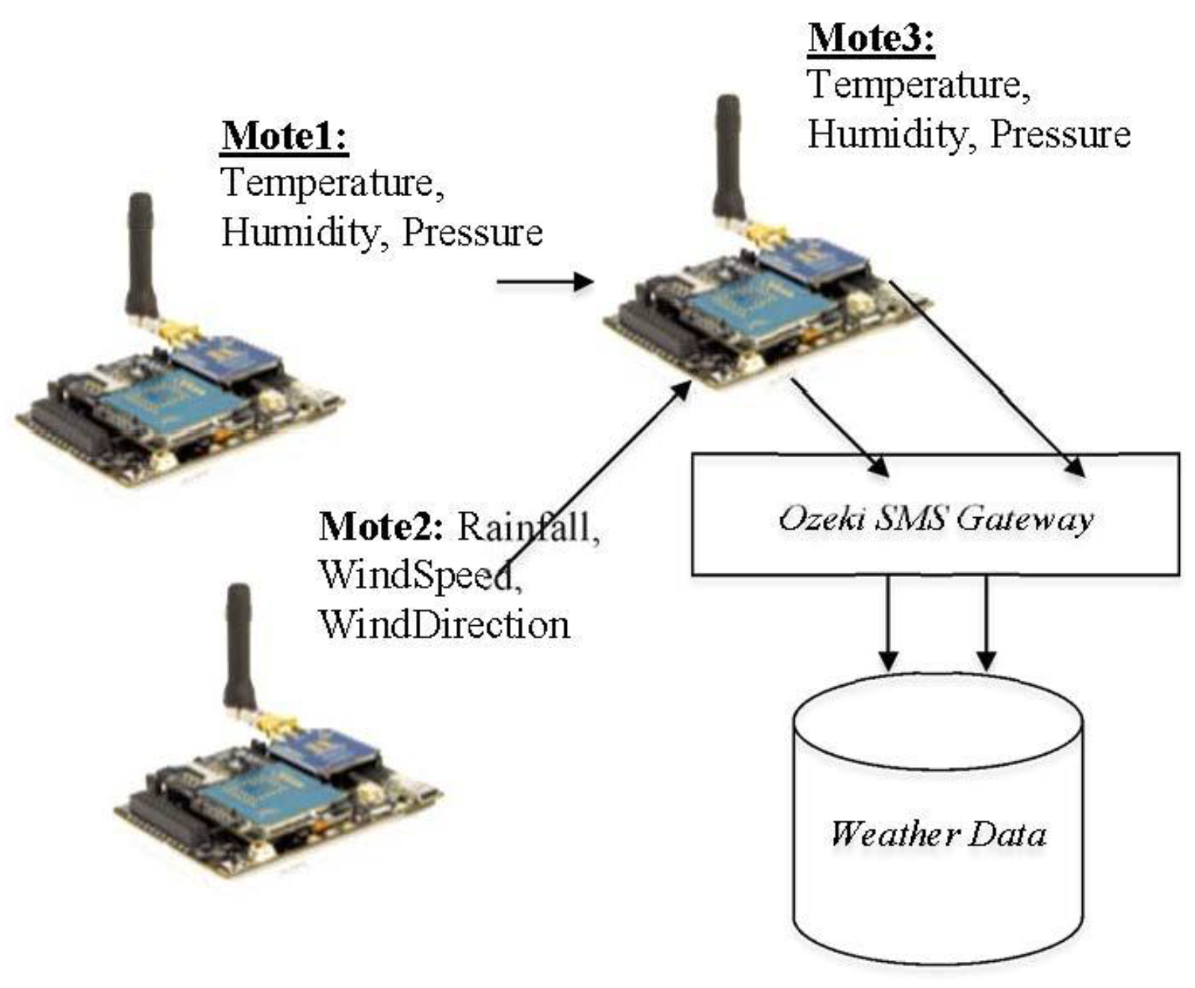
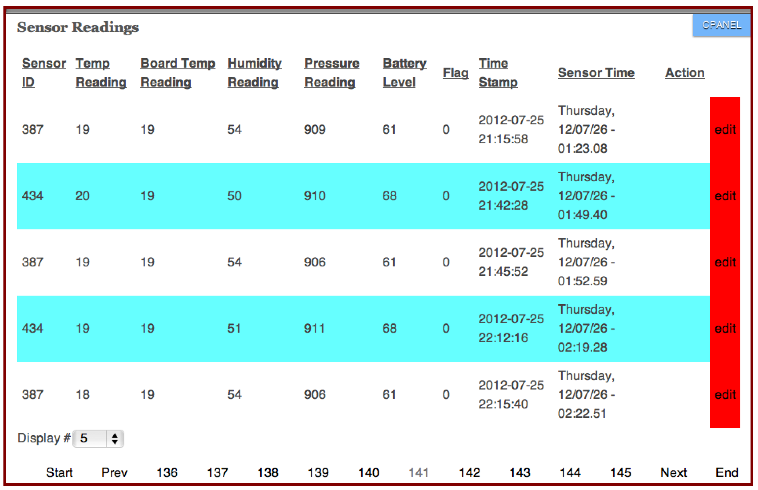
3.3. Aggregating Sensors Readings

The sensors were programmed to take readings every 30 min, while the readings from the weather station were taken on hourly basis. That is, at hour t (say 1 GMT), the sensor boards recorded two readings for each of the sensors, for example with 6 sensor boards, each fitted with 3 sensors (temperature, humidity and pressure); this would result in 12 readings for temperature, 12 readings for humidity and 12 readings for pressure. In order to aggregate these readings for the purpose of comparing them with the respective readings from the weather station, the following two options were pursued:

(I)

Option 1: average all sensor readings taken within the hour:

$$S_s=\frac{{\displaystyle \sum _{i=1}^n(S_{i1}+S_{i2})}}{2n}$$

(1)

where S_s is the aggregated reading for Sensor S; for example, S could be a temperature sensor or humidity sensor. S_i1 and S_i2 are the sensor reading for Sensor S on Sensor Board i (see Equation (1) above). For instance, in the case of five sensor boards, the aggregated reading for temperature sensors would be computed as shown in Equation (2)

$$S_s=\frac{T_{1,1}+T_{1,2}+T_{2,1}+T_{2,2}+T_{3,1}+T_{3,2}+T_{4,1}+T_{4,2}+T_{5,1}+T_{5,2}}{10}$$

(2)

(II)

Option 2: average readings taken closest to the hour:

In this case, only one out of the two sensor reading from each sensor board is considered; the one closest to the weather station readings’ observation time (Equation (3)). That is:

$$S_s=\frac{{\displaystyle \sum _{i=1}^n(S_{i1})}}{n}$$

(3)

This implied, given five sensor boards, the aggregated reading for the temperature sensor would be:

$$T_s=\frac{T_1+T_2+T_3+T_4+T_5}{5}$$

(4)

3.4. Equipment Selection

Wireless sensor network application in weather monitoring is still relatively new, and most of the boards do not meet the minimum parameter requirement set by the World Meteorological Organization. These are listed in [8] as: (1) precipitation (type and amount); (2) surface air temperature; (3) atmospheric pressure; (4) wind direction and speed; and (5) relative humidity. Most sensor boards reviewed were found to lack support for (1) and (4). Libelium’s Agriculture Board supports all of these and more (Figure 2).

Figure 2. Anatomy of agriculture sensor board PRO. LWS (leaf wetness sensor).

Figure 2. Anatomy of agriculture sensor board PRO. LWS (leaf wetness sensor).

This board supports the following sensors:

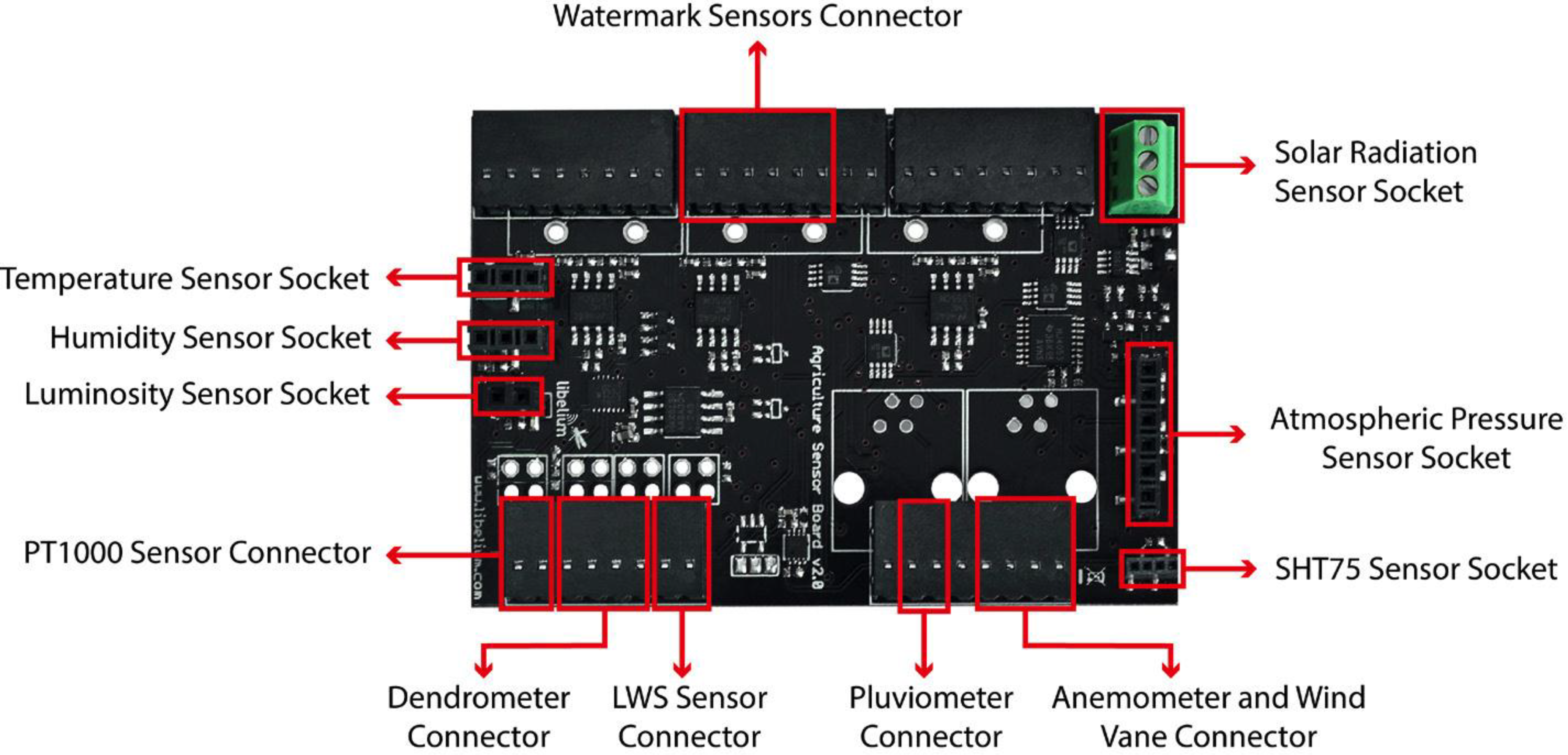
• Temperature sensor MCP9700A by Microchip;
• Humidity sensor 808H5V5 by Sencera;
• Temperature and humidity sensor SHT75 by Sensirion;
• Soil moisture sensor Watermark by Irrometer;
• Atmospheric pressure sensor MPX4115A by Freescale;
• Leaf wetness sensor (LWS);
• Solar radiation sensor SQ-110 by Apogee;
• DC2, DD and DF dendrometers by Ecomatik;
• Soil temperature sensor PT1000;
• EWeather Station (anemometer, wind vane and pluviometer).

Other supporting sensors and accessories that were used are:

• Lithium batteries, for power supply;
• General packet radio service (GSM)/Global System for Mobile Communications (GPRS) module, for sending data via the mobile telephone network;
• GPS receiver, for getting GPS coordinates (latitude, longitude, height, speed, direction, date/time and ephemerids); this is to enable support for mobile data sensing;
• SD cards, for data storage;
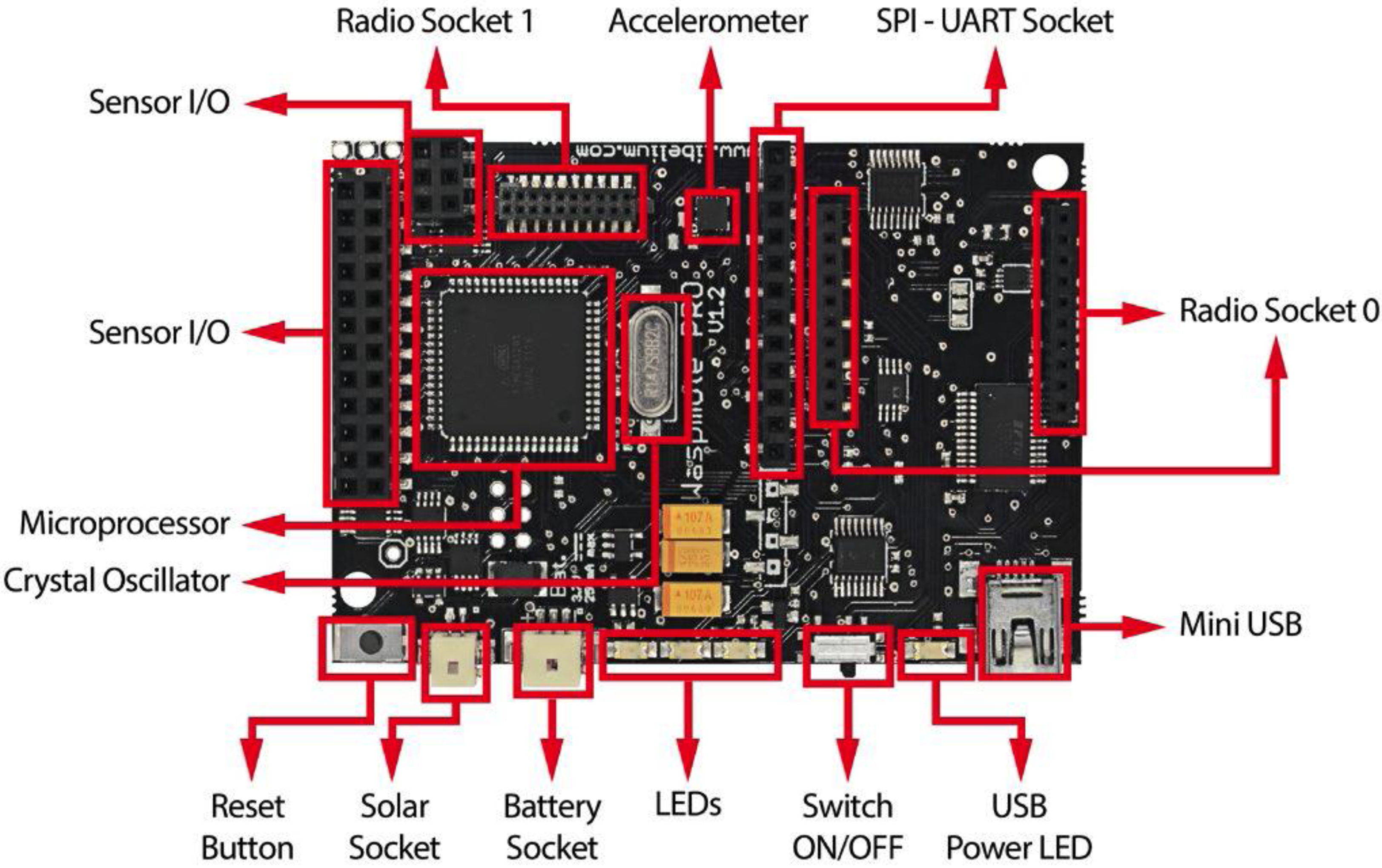
• USB cables for uploading program to the Waspmotes;
• Waspmote gateway, XBee radio and XBee antennas (2 dBi/5 dBi) for networking the sensor nodes.

The above were mounted on the Waspmotes shown below (Figure 3).

Figure 3. Anatomy of the Waspmote

Figure 3. Anatomy of the Waspmote

The work described here was geared towards calibrating a few (list in Table 1) of the sensors above against the respective weather instruments.

Table 1. Details of the sensor equipment used.

Weather Parameter	Sensor Board	Weather Instrument
Temperature	Temperature sensor MCP9700A by Microchip	Mercury-in-glass thermometer
Relative Humidity	Humidity sensor 808H5V5	Computed using a humidity slide rule
Atmospheric Pressure	Atmospheric pressure sensor MPX4115A by Freescale	Kew-type station barometer:

Table 1. Details of the sensor equipment used.

Weather Parameter	Sensor Board	Weather Instrument
Temperature	Temperature sensor MCP9700A by Microchip	Mercury-in-glass thermometer
Relative Humidity	Humidity sensor 808H5V5	Computed using a humidity slide rule
Atmospheric Pressure	Atmospheric pressure sensor MPX4115A by Freescale	Kew-type station barometer:

In preparing the sensors for the real world, enclosures were designed; a sample is shown below (Figure 4).

Figure 4. Sensor board enclosures.

Figure 4. Sensor board enclosures.

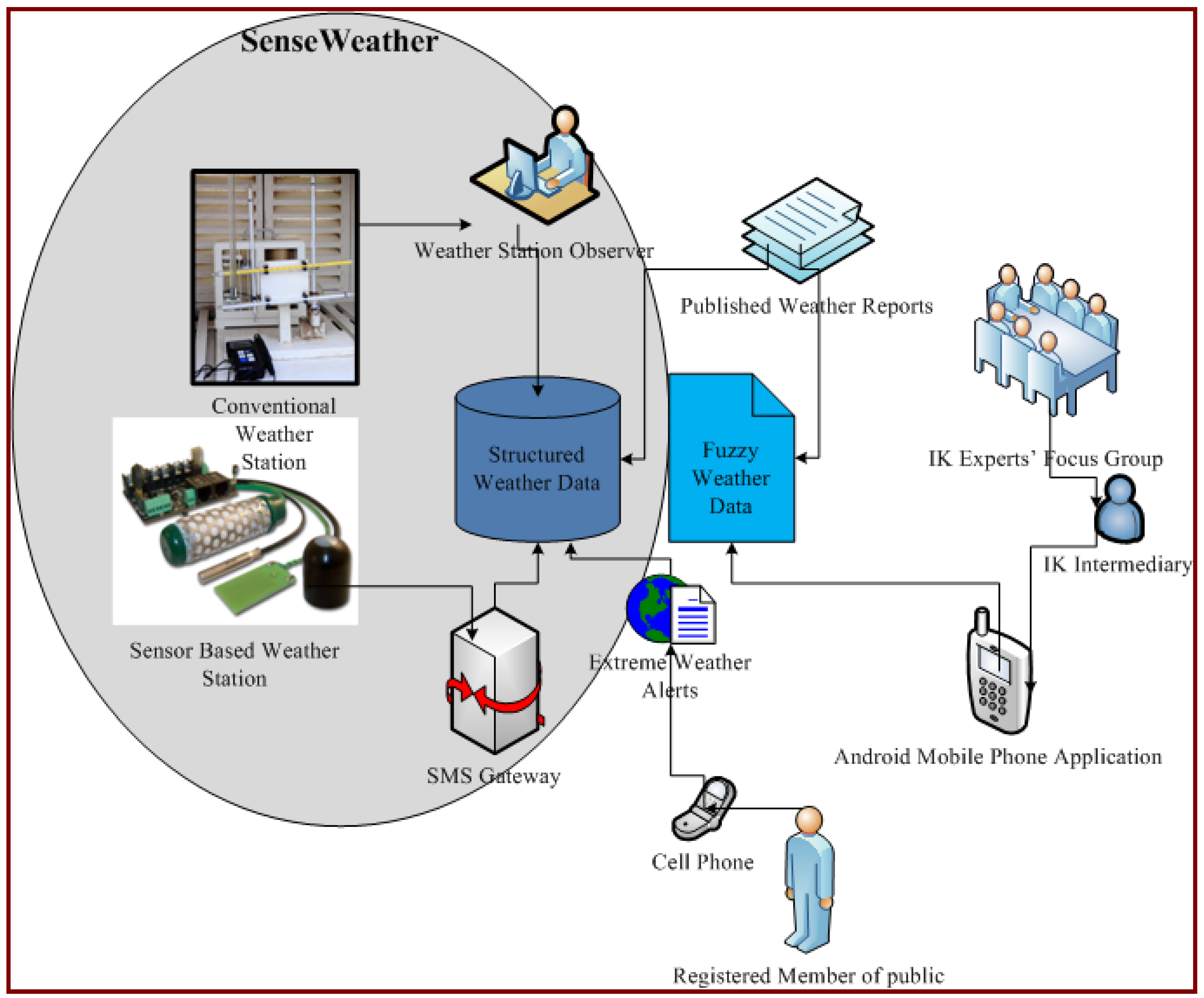
3.5. SenseWeather System Design and Implementation

SenseWeather is part of a comprehensive DEWS [13] made up of several sub-systems that are linked up together by intelligent agents that were implemented using the Java-based multi-agent systems’ development framework called JADE (Java Agent Development). The sub-systems are: (1) the Sensor-Based Weather Monitoring System prototype (SenseWeather); (2) the Effective Drought Index (EDI) monitor, which is a FORTRAN program; (3) ANNs forecasting tool; (4) the IK Fuzzy Sub-System that stores indigenous knowledge (IK) drought indicators; (5) the Android Mobile Application to input and output IK indicators, as well as extreme weather events; (6) the SMS gateway that allows members of the public to interact with the entire system and also used to receive weather readings from sensors into the system; and (7) a user-friendly web portal used for both system administration, as well as for displaying detailed information on droughts and other related details.

The integrated system was designed to meet the need for an affordable, relevant, sustainable and user-friendly drought early warning system (DEWS) for Sub-Saharan Africa. This DEWS is currently implemented under a framework called ITIKI (Information Technology and Indigenous Knowledge with Intelligence), which is a bridge that integrates the indigenous drought forecasting approach into the scientific drought forecasting approach. Some of the relevant (to this paper) sub-systems of the integrated system logic are captured in the figure below (Figure 5).

Figure 5. SenseWeather: system logic. IK, indigenous knowledge.

Figure 5. SenseWeather: system logic. IK, indigenous knowledge.

Two types of deployments of SenseWeather were set up:

(1)

Sensor boards next to weather stations:

Here, sensor boards were placed within the Observatory Units of selected weather stations in Kenya. The boards individually send readings to a remote database via an SMS gateway. The sensors included are those for measuring temperature, relative humidity and atmospheric pressure. In a few of the locations, rainfall, wind speed, wind direction and soil moisture sensors were installed. Aggregation of multiple sensor readings was performed using Option 2 described under the Calibration Section 3.3. Apart from monitoring weather, this setup sought to further validate the calibration decisions.

(2)

Stand-alone sensor boards:

In order to deploy the sensors in the rural areas, especially in Mbeere and Bunyore (in Kenya), on which SenseWeather deployments were targeted, stand-alone sensors mounted with temperature, relative humidity and atmospheric sensors were used. The sensor boards were placed inside traditional granaries, which provided an environment almost similar to the one supported by the Stevenson screens.

A wireless sensors network made up of 3 nodes was designed and implemented as follows (Figure 6).

Figure 6. Wireless sensor network design.

Figure 6. Wireless sensor network design.

Figure 7. Sensor board monitoring interface.

Figure 7. Sensor board monitoring interface.

In the implementation, program code that puts into consideration the calibration weights reached during the calibration exercise was loaded on to each of the sensor boards; readings were then taken every 30 min. To minimize the cost of sending SMS, the sensors send the readings to the database (using the GSM/GPRS module) via the SMS gateway on an hourly basis. For backup purposes, each board also saves all (every 30 min) of the readings in a secure digital (SD) card. The activity of the sensors is monitored from a web interface; a sample is shown in Figure 7.

4. Results and Discussion

4.1. Reading Time Lags (Lag Errors)

Though programmed to sleep for 30 min, the sensors had time lags due to various computation tasks, especially: delay statements used for stabilizing power supply after waking up, writing to SD cards, print and println statements and GPRS commands. These time lags ranged between 8 and 47 s, and this kept on increasing as the size and number of output files (text files used to store the readings within the boards’ SD cards) increased. Since this would render the readings unacceptable by the World Meteorological Organization, which allows a maximum of a 15-min delay, the lags were resolved through re-programming the sensor boards. For example, given that, on average, the sensor had a time lag of 8.645 s, an adjustment of 7 s was factored into its sleeping time:

const * sleep_duration = “00:00:30:00”; to: const * sleep_duration = “00:00:29:53”

4.2. Sensor vs. Weather Station Data Analysis

As explained under Section 3.3, given that sensor boards were fitted with three sensors each—temperature, humidity and pressure—and that each sensor took readings every 30 min, each sensor had two readings for each parameter per hour. On a given date and time (say 10 October 2011 at 15:00), the sensors would output six temperature readings: two from each temperature sensor mounted on each of the three sensor boards. In order to compare these with the equivalent hourly readings from the weather station, aggregation of the values for each parameter were computed using Option 1 and Option 2 described in Section 3.3. Below is an illustration of the error analysis carried under Option 1 (Table 2).

(a)

Error Analysis

Table 2. Comparison of Option 1 error analysis.

Error Type	Temperature Sensor	Humidity Sensor	Pressure Sensor
ME	1.54	6.52	−12.80
MAPE	8.21%	9.58%	1.35%
RMSE	1.63	8.31	12.83

Table 2. Comparison of Option 1 error analysis.

Error Type	Temperature Sensor	Humidity Sensor	Pressure Sensor
ME	1.54	6.52	−12.80
MAPE	8.21%	9.58%	1.35%
RMSE	1.63	8.31	12.83

(b)

Sensor Readings Adjustments

Three options of adjusting the errors in the table above were carried out by applying ME, MAPE and RMSE; the adjustments using MAPE had the greatest gradient and, therefore, was adopted for the final adjustment, as shown in the expression below:

AdjustedTempt = OriginalTempt + (OriginalTempt * MAPE/100)

The adjusted temperature reading for each sensor taken at time t was then computed by adding a weight factor equivalent to the respective mean absolute percentage error. That is, 8.21%, 9.58% and 1.35% for temperature, humidity and pressure, respectively. These changes were effected on the entire dataset after which the process of computing the errors was then repeated, resulting in the following values (Table 3).

Table 3. Option 1 error analysis after MAPE factor adjustment.

Error Type	Temperature Sensor	Humidity Sensor	Pressure Sensor
ME	0.08	1.04	0.17
MAPE	3.35%	6.14%	0.08%
RMSE	0.74	4.30	0.87

Table 3. Option 1 error analysis after MAPE factor adjustment.

Error Type	Temperature Sensor	Humidity Sensor	Pressure Sensor
ME	0.08	1.04	0.17
MAPE	3.35%	6.14%	0.08%
RMSE	0.74	4.30	0.87

(c)

Similarity Tests

In order to graphically view the similarities between sensor and station readings, graphs similar to the one in Figure 2 below were plotted for both before and after the MAPE adjustments described above (Figure 8).

Figure 8. Comparison between the humidity sensor (in enclosures) and the station.

Figure 8. Comparison between the humidity sensor (in enclosures) and the station.

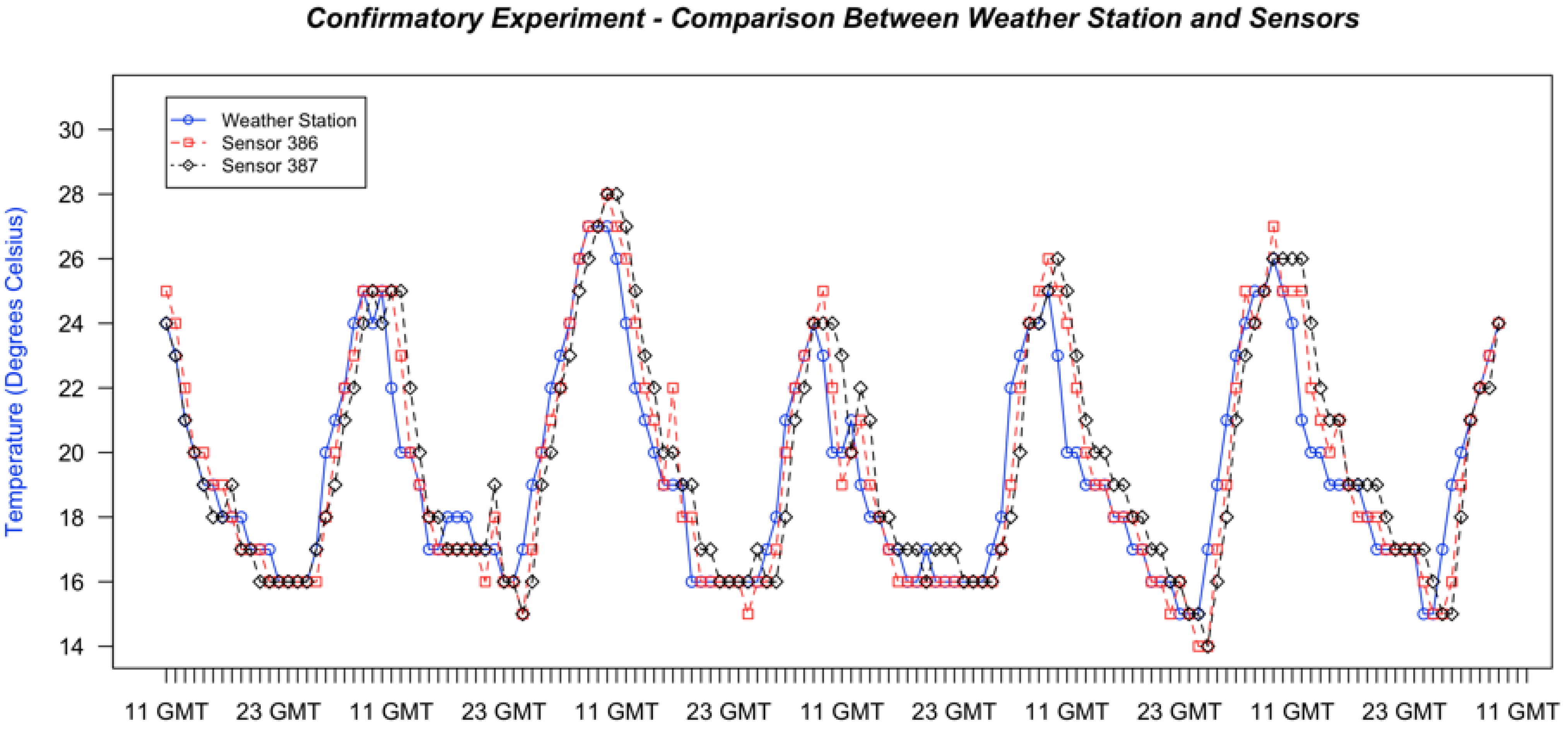
4.3. Confirmatory Experiments

After all of the necessary adjustments during the exploratory experiments were effected, a confirmatory experiment was carried out. The objectives here were to first “confirm” that the adjustments proposed were the best and, two, to choose between the two options (Options 1 and 2) of aggregating sensor readings. As with exploratory experiments, the adjustments were factored into the program code and loaded onto the sensors.

Example, temperature sensor: the individual errors for each board were used:

//Factor in MAPE of 8.21% = 0.0821
value_temp = value_temp + (value_temp * 0.0821)

Before reaching the final decision as to which of the two options (of combining sensor data) to use, further analyses were carried out as explained below (Table 4).

(a)

Error Analysis

Table 4. Confirmatory experiment: error analysis summaries.

Error Type	Option	Temperature	Humidity	Pressure
MAPE	Option 1	8.55	12.54	1.47
	Option 2	8.53	11.90	1.47
RMSE	Option 1	1.96	10.94	12.06
	Option 2	1.89	10.56	12.10

Table 4. Confirmatory experiment: error analysis summaries.

Error Type	Option	Temperature	Humidity	Pressure
MAPE	Option 1	8.55	12.54	1.47
	Option 2	8.53	11.90	1.47
RMSE	Option 1	1.96	10.94	12.06
	Option 2	1.89	10.56	12.10

For temperature and humidity sensors, Option 2 performed better for both MAPE and RMSE. However, though Options 1 and 2 had equal performance (1.47) for the pressure sensor using MAPE, Option 1 outperformed Option 2 under RMSE (12.06 vs. 12.10). Based on some discrepancies noted for the pressure readings during the experiments (the details are discussed in the Further Work Section), the discrepancy above was ignored, and a decision to pick Option 2 as the best way of combining the sensor readings was reached.

(b)

Correlation Coefficients

To further validate the choice of Option 2, the correlation coefficients of the sensor readings with the weather station were computed (Table 5).

Table 5. Confirmatory experiment: correlation coefficients.

Options	Temperature	Humidity	Pressure
Option 1	0.924	0.920	0.723
Option 2	0.940	0.936	0.657

Table 5. Confirmatory experiment: correlation coefficients.

Options	Temperature	Humidity	Pressure
Option 1	0.924	0.920	0.723
Option 2	0.940	0.936	0.657

Again, except for the pressure sensor, Option 2 had the highest correlation coefficients.

4.4. Calibrating the Sensors

Using Option 2, the MAPE error factors of 8.53% and 11.90% for temperature and humidity respectively were used to calibrate the sensors. These values were used to update the program code as follows:

value_temp = value_temp + (value_temp * 0.0853)

value_humid = value_humid + (value_humid * 0.119)

Similarly, though not the lowest, the pressure MAPE value (1.47) for Option 2 was used. The decision was reached for uniformity purposes and also the fact that the Option 1 value (1.46) was close to this one. The code therefore looked like this:

value_pressure = value_pressure − (value_pressure * 0.0147)

4.5. Battery Tests

The sensor boards employed in this research made use of chargeable lithium batteries for power. In order to determine how often to charge/replace the batteries, a series of experiments were performed to answer the following questions: (1) How long does it take to charge a battery that is almost depleted? (2) How long does a fully charged battery run when used on a sensor board with various sensors installed and under different operation modes (for example, sleep_mode ON or OFF)? (3) How do various environmental conditions (cold, rainy, hot, and so on) under which the sensor boards are operating affect the batter power?

Figure 9. Battery power management: recharge curve.

Figure 9. Battery power management: recharge curve.

Figure 10. Battery power management: discharge curves.

Figure 10. Battery power management: discharge curves.

Some of the results attained (shown in Figure 9 and Figure 10 above) included: (1) it took an average of twenty hours to fully charge a battery that was almost completely depleted; (2) a battery powering a sensor board that has four sensors (temperature, humidity, pressure and GPRS) and set to operate with SLEEP_MODE (wakes up every 30 min to take readings) set to ON would use up to 60% of the battery power within one week, and it would take about 24 h to reach the same battery level with SLEEP_MODE set to OFF; (3) at about 38% power level, a battery would experience problems powering the GPRS; and (4) as expected, re-charging and discharging of the batteries curves are linear. The discharging curve, however, is not smooth; the batteries seem to “gain” some power when put into sleep mode and sharply lose power due to the nature of the sensors (especially GRPS) mounted on the boards.

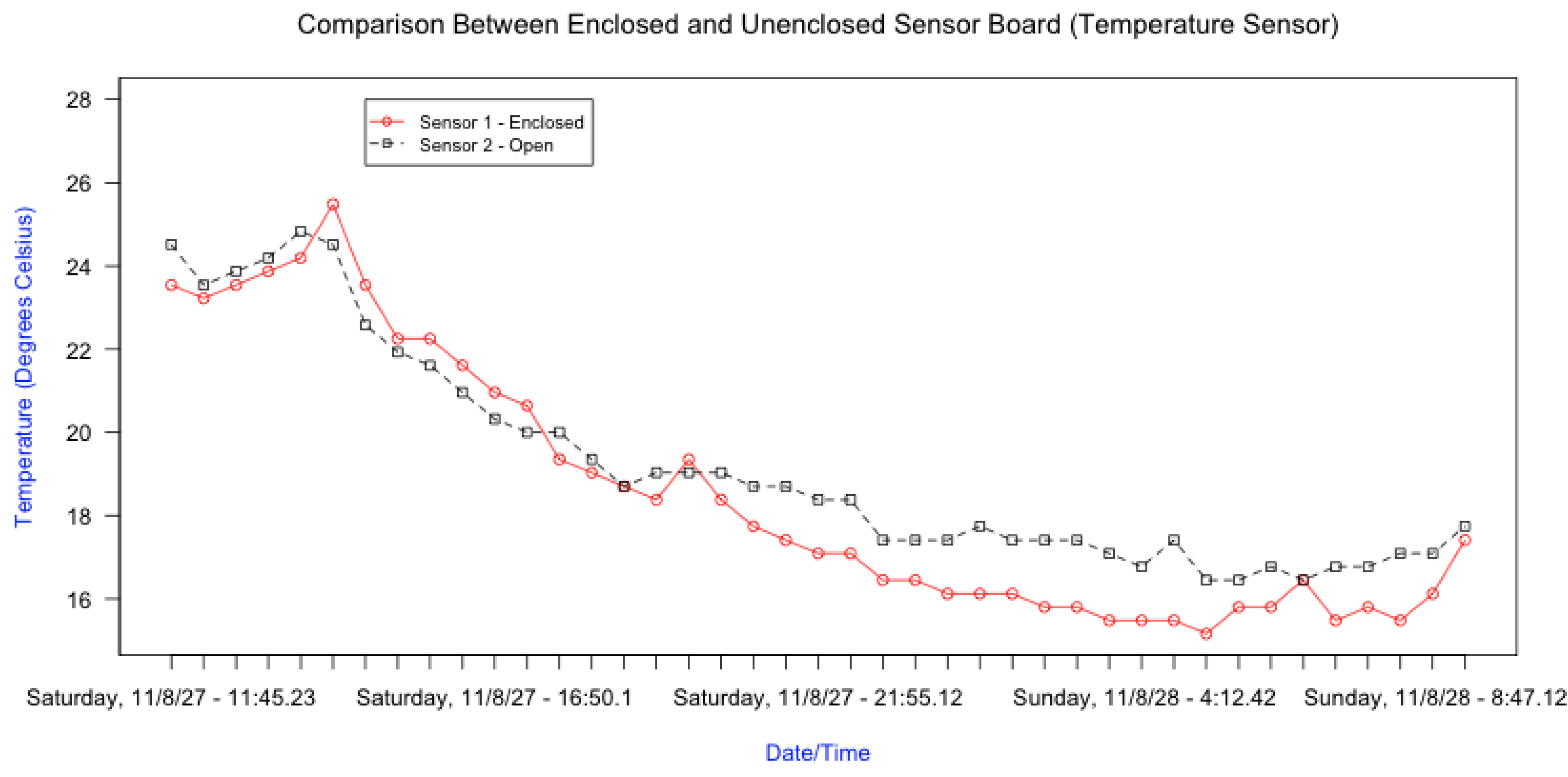
4.6. Sensor Board Enclosure

Temperature sensor: Though the majority of the readings from the two sensors was similar (correlation value of 0.98), the enclosed sensor had some erratic readings as shown in Figure 11 and Figure 12 below. In the course of the experiments, it was established that sensor board temperature taken using the function int boardTemp = RTC.getTemperature() could be used to take care of scenarios where the temperature sensor gives erroneous readings. This was therefore used to eliminate the few enclosed temperature sensor outliers.

Humidity Sensor: Similarly, the majority of the readings from the two sensors was similar (correlation value of 0.97). However, the probability of the enclosed humidity sensor to give erroneous readings (correlation of 0.32) increased with time; this was associated wetness within the enclosure. After 48 h, for instance, the relative humidity readings ranged between 113% and 114%.

Pressure Sensor: This sensor consistently generated erroneous readings. The readings remained at 16.93 and, therefore, comparisons between the sensor reading and those from the weather station were not performed.

Figure 11. Behavior of temperature sensors in and outside of Perspex enclosures.

Figure 11. Behavior of temperature sensors in and outside of Perspex enclosures.

Figure 12. Behavior of relative humidity sensors in and outside of Perspex enclosures.

Figure 12. Behavior of relative humidity sensors in and outside of Perspex enclosures.

5. Conclusions and Further Work

5.1. Inherent Sensor Board Facts

When using the Libelium’s Agriculture sensor boards programmed to sleep for 30 min and write up to a maximum of 160 (standard SMS length) characters into output files stored in an SD card, it emerged that the board will spend an average of 7 s in “waking up” (delay (100) for stabilizing power supply after waking up) and I/O operations (writing to SD card and println statements). Since this happens at every reading, this error cumulatively becomes very significant and may render the time-sensitive weather readings unusable. The value seemed to increase as the size of the output file (an increase by 1 s on the 78th line and 2 s after the 178th line) grew. Depending on how large this file is, the following code could be used to counter this delay:

const * sleep_duration = “00:00:29:53”; in place of: const * sleep_duration = “00:00:30:00”

Further, with a sensor board that writes into two output files (30 and 60 min, respectively) and also sends an SMS after every 60 min, an average delay of 42 s per hour will be experienced. This can be addressed by writing:

const * sleep_duration = “00:00:29:40”; instead of const * sleep_duration = “00:00:30:00”

The code above does not entirely eradicate the time lags; by Day 7, sensor boards with GPRS activated will have cumulative time lags of 500 s, while those without GPRS will have 50-s time lags. The author recommends that the sensors should be reset after every seven days to avoid scenarios where these time lags delay the sensor readings by values greatly above the WMO recommended limits (15 min).

5.2. Appropriate Material for Building Sensor Enclosures

The design of the enclosures for the sensor boards to be used for weather monitoring must be addressed/tackled using meteorological science approaches. They must meet strict specifications in order to ensure that they represent a true natural environment just the way the Stephen screen does. An attempt to use Perspex to design an enclosure for this research, for example, caused the humidity sensor to fail.

5.3. Future Work

The very nature of the sensors and the observation methods of their readings pose some challenges and questions for meteorologists. Unlike manual weather stations that are commonly used in SSA, the operation of sensors-based weather stations is highly automated; for instance, readings can be taken and stored in a database at a very high frequency (seconds) if need be. The challenge here is that in determining the “best” reading for a given hour (say 6 GMT), is it better to just report the reading taken at 5:59 GMT or that the cumulative readings are taken throughout the hour. Further, the weather station readings used to calibrate the sensors were those from a manual weather station, and since a human operator takes these readings, the readings might not have been as accurate as expected. Different sets of experiments are needed in order to compare the sensor readings with values read from an automatic weather station.

The sensor boards described in this paper are not ready for use in the field until an enclosure designed with the input of meteorologists is completed. The enclosure should take into consideration all of the WMO recommended specifications, such as the angle of elevation and the effect of using the enclosure in motion (mounted on a moving vehicle). In line with this, other weather sensors (for precipitation, wind speed and direction and soil moisture) should be calibrated during the next phase of the project. Finally, more sensor boards (Agriculture boards) have been procured to run more confirmatory sets of experiments and to further confirm the error factors reached. Once this is done, the researcher will then approach the relevant authorities at WMO for the appropriate standardization process.

References

1. Armstrong, S.; Mark, C.; Randolph, K.; Dan, M. World Disasters Report—Focus on Hunger and Malnutrition, 1st ed.; International Federation of Red Cross and Red Crescent Societies: Geneva, Switzerland, 2013. [Google Scholar]
2. Patt, A.G.; Jordan, W. Applying Climate Information in Africa; An Assessment of Current Knowledge. Available online: http://www.iiasa.ac.at/Publications/Documents/XO-07-006.pdf (accessed on 2 February 2015). Written in Support of NOAA, Boston University and the International Institute for Applied Systems Analysis (IIASA)
3. Masinde, M.; Bagula, A.; Muthama, N. Wireless Sensor Networks (WSNs) use in Drought Prediction and Alerts. In Application of ICTs for Climate Change Adaptation in the Water Sector: Developing Country Experiences and Emerging Research Priorities. APC, IDRC, CRDI; Finlay, A., Adera, E., Eds.; Association for Progressive Communication (APC) and the International Development Research Centre (IDRC): Johannesburg, South Africa, 2012; pp. 107–108. [Google Scholar]
4. Abdoulie, J.; John, Z.; Alpha, K. Climate Information for Development Needs: An Action Plan for Africa—Report and Implementation Strategy; World Meteorological Organization (WMO): Geneva, Switzerland, 2006. [Google Scholar]
5. EAC, S. Enhancing Capacities of the Meteorological Services in Support of Sustainable Development in the East African Community Region Focusing on Data Processing and Forecasting Systems. Available online: http://www.eac.int (accessed on 2 April 2014).
6. Masinde, M.; Bagula, A. ITIKI: Bridge between African indigenous knowledge and modern science of drought prediction. Knowl. Manag. Dev. J. 2012, 7, 274–290. [Google Scholar] [CrossRef]
7. Libelium, Comunicaciones Distribuidas, S.L. Agriculture Board Technical Guide. 2010. Available online: http://www.libelium.com (accessed on 2 February 2015).
8. Plummer, N.; Terry, A.; José, A.L. Guidelines on Climate Observation Networks and Systems; World Meteorological Organization: Geneva, Switzerland, 2003. [Google Scholar]
9. Manual on the Global Observing System: Volume I (Annex V to the WMO Technical Regulations); World Meteorological Organisation: Geneva, Switzerland.
10. Jarraud, M. Guide to Meteorological Instruments and Methods of Observation (WMO-No. 8); World Meteorological Organisation: Geneva, Switzerland, 2008. [Google Scholar]
11. Eisenhart, C.; Dorsey, N.E. On Absolute Measurement. The Sci. Mon. 1953, 77, 103–109. [Google Scholar]
12. Phillips, S.D.; Estler, W.T.; Eberhardt, K.R.; Levenson, M.S. A careful consideration of the calibration concept. J. Res. National Inst. Stand. Technol. 2001, 106, 371–379. [Google Scholar] [CrossRef]
13. Masinde, M. An innovative drought early warning system for sub-Saharan Africa: Integrating modern and indigenous approaches. Afr. J. Sci. Technol. Innov. Dev. 2015, 7. [Google Scholar] [CrossRef]
14. Guidelines for National Meteorological Services in the Establishment of National Climate Services; World Meteorological Organisation: Geneva, Switzerland, 12 May 2014.