4.1. Definitions
First, we introduce some definitions:
∘ D5. Primary schedule: is the initial optimized time slot assignment obtained with MODESA; it includes only slots needed by regular messages. These slots are said to be regular. Consequently, the number of regular slots granted to any ordinary node is equal to the sum of its initial demand and the initial demands of all its descendants.
∘ D6. Bonus slot: is a temporary slot assigned after a change notification (e.g., temporary change in the application need, retransmission, etc.).
∘ D7. Secondary schedule: is the optimized assignment of bonus slots obtained with AMSA.
∘ D8. Slot path: is a sequence of slots that allows the transmission of a message from any given ordinary node to the sink.
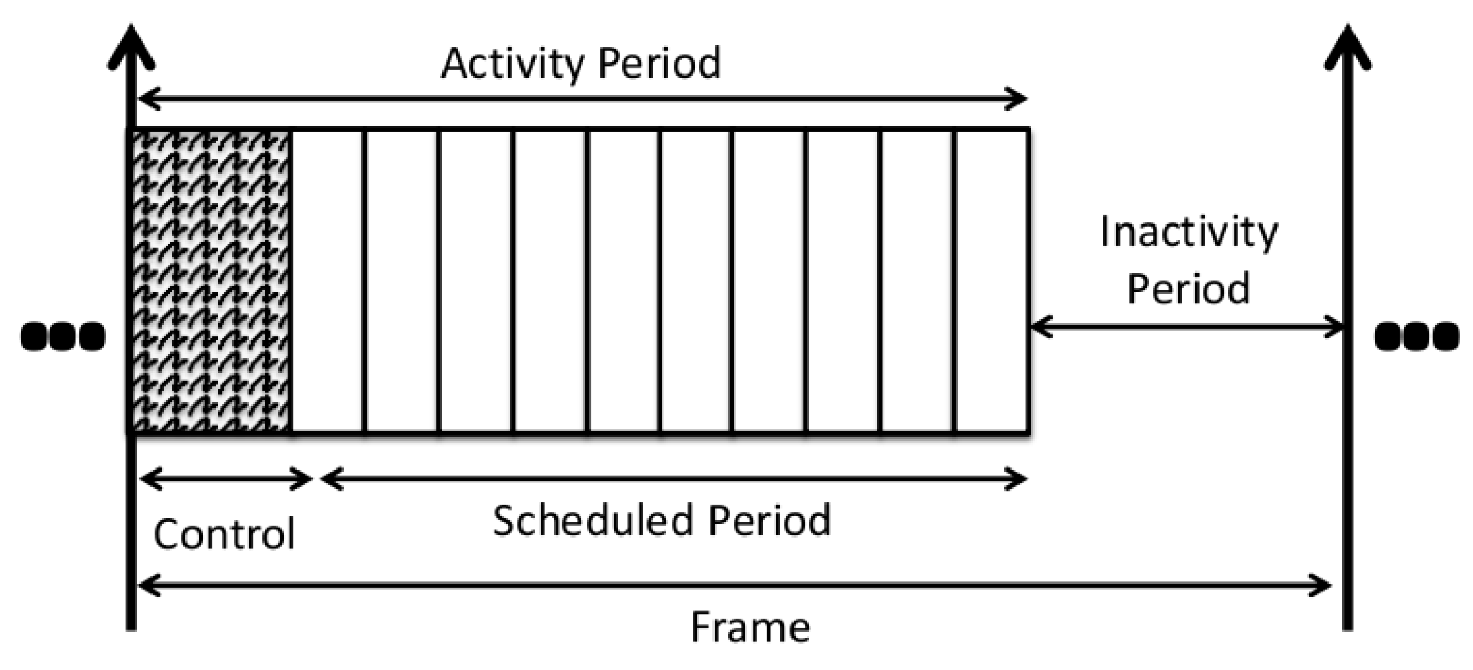
∘ D9. Extra slot: is a bonus slot that is appended at the end of the primary schedule. Any extra slot increases the length of the activity period.
∘ D10. Complementary schedule: is the optimized time slot assignment obtained with MODESA taking into account only the requests of bonus slots. It starts at the end of the primary schedule.
4.3. Model
The network is formalized as a graph, , where is the set of vertices representing the nodes of the network and is the set of edges representing the communication links between the nodes.
Let , where is the set of ordinary nodes and represents the set of sinks, with . For each node, , we define , the set of conflicting nodes that interfere with v when transmitting on the same channel. Moreover, let denote the number of physical interfaces available at any node, v. For any ordinary node, , let correspond to the number of bonus slots requested by n to transmit the additional packets it generates.
Let denote the set of links through which a node, v, can transmit. Let be the set of links through which a node, v, can receive. For any link, , let denote the number of slots needed to transmit over the link, e, the additional packets generated by node, n.
Let be the set of channels usable for any transmission. The collision-free period is composed of slots, t, in the interval, , where denotes an upper bound of the frame length. This bound is reached when all packets are sent sequentially on the same channel. We then have: , where is the depth of node, n, in the data gathering tree.
Let the parameter correspond to the activity of a link, e, on the channel, c, in the time slot, t, in the primary schedule, i.e., , if and only if there is a transmission of a packet on the link, e, on the channel, c, in the time slot, t, in the primary schedule, and , otherwise. This binary parameter is given by the MODESA algorithm.
We define as bonus slot assignment for a link, e, on the channel, c, in the time slot, t, i.e., , if and only if there is a transmission of a packet on the link, e, on the channel, c, in the time slot, t, in the bonus assignment, and , otherwise.
Furthermore, let be the use of a slot, t, in other words, means that there is at least one link activity (activity in the primary or secondary schedule) on at least one channel in the slot, t, and denotes an empty slot.
Table 1 summarizes the inputs and variables of our model.
Table 1.
Inputs and variables of the model.
Table 1.
Inputs and variables of the model.
| Inputs |
| set of links in the topology |
| set of nodes in the topology |
| set of available channels |
| number of interfaces of the node, v |
| set of nodes conflicting with v |
| number of bonus slots requested by node, n |
| activity of the link e in time slot, t, on channel, c, |
| Variables |
| utility of slot, t |
| number of slots needed to transmit over link, e, the additional packets generated by node, n |
| assignment of bonus slot, t, to link, e, on channel, c, |
The objective is to minimize the number of slots,
:
with the following constraints:
Constraint 1 binds the use of a time slot to at least the activity of one link on any channel in this slot in the primary schedule or the secondary schedule.
Constraint 2 guarantees that a node cannot transmit while one of its conflicting nodes is already scheduled in the same slot on the same channel in the primary schedule.
Constraint 3 ensures that for the bonus slot assignment, two conflicting nodes do not transmit on the same channel in the same time slot.
Constraint 4 limits the number of simultaneous communications for a node, during the primary schedule and the bonus assignment, to its number of interfaces.
Constraint 5 ensures the mapping between the activities on all channels and the packets sent on links.
Constraints 6–8 express the conservation of messages, respectively, at the nodes requesting a bonus slot, at intermediate nodes and at the sinks.
Constraint 9 makes certain that a packet is generated or received by a node before being transmitted or forwarded.
Notice that this model can be applied to compute the primary schedule by setting
4.4. Theoretical Bounds on the Number of Extra Slots for a Raw Data Convergecast
We now provide lower and upper bounds for the number of extra slots added after the regular ones by any incremental solution. This should preserve the primary schedule and ensure that the data gathering, including the additional demands, is performed in a single frame.
Property 1 The minimum number of extra slots is given by the difference between, on the one hand, the optimal slot assignment meeting for each node the sum of its initial and the new demands and, on the other hand, the number of regular slots.
Proof: The number of slots required by the incremental algorithm is the sum of regular slots and extra slots. In the best case, this sum is equal to the number of slots obtained by the optimal algorithm to schedule both initial and new demands. Hence, the minimum number of extra slots is the difference between the number of slots given by the optimal algorithm and the number of regular slots. ■
Property 2 The maximum number of extra slots is given by , where is the depth of any ordinary node, u, in the convergecast tree and is the number of bonus slots requested by u.
Proof: The maximum number of extra slots added to the regular ones corresponds to the worst case, which occurs when there is no parallelism between the slot paths granted, corresponding to the additional demands. It is given by , where is the depth of any ordinary node, u, in the convergecast tree; it is also the length of the path from this node to the sink, and is the number of bonus slots requested by u. ■
We can improve this upper bound, by taking into account some parallelism in the transmissions. We then get:
Property 3 The maximum number of extra slots is given by the , where is the maximum depth in the convergecast tree of any ordinary node requesting bonus slots, is the number of bonus slots requested by any ordinary node, u, and is defined as follows: | = | | if is even, |
| | = | | otherwise, |
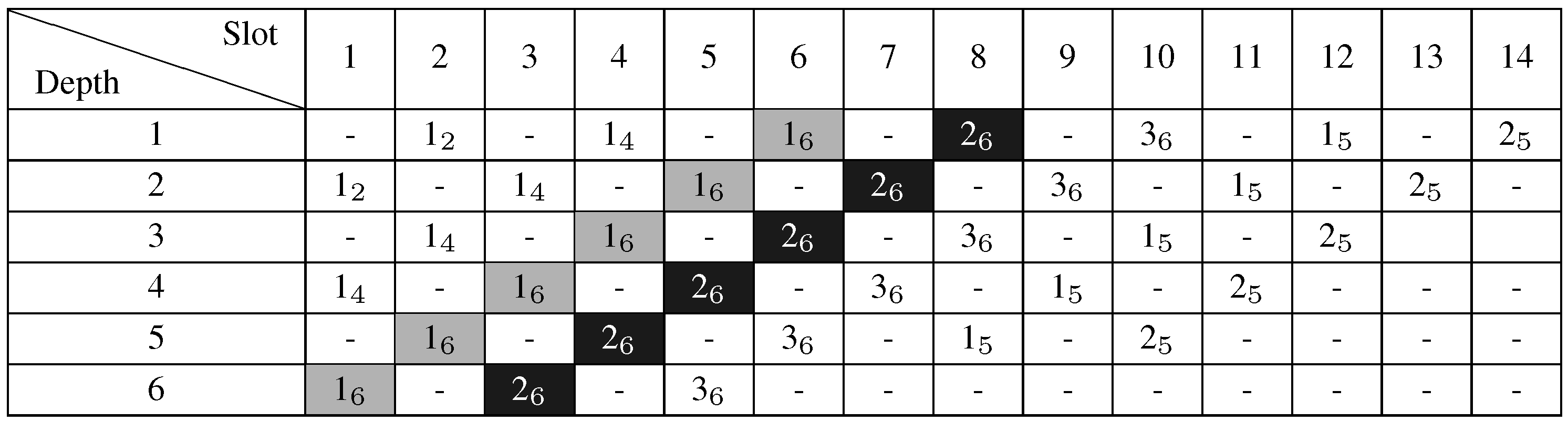
with = 1, if and only if there is at least one node, u, of depth, k, requesting bonus slots. Proof: We now build a schedule for all the requests for bonus slots. Like AMSA, this schedule assigns slots per path from the requesting node to the sink. Let
u be the node with the greatest depth in the convergecast tree requesting bonus slots. Let
be its depth. If scheduled first, node
u, will require
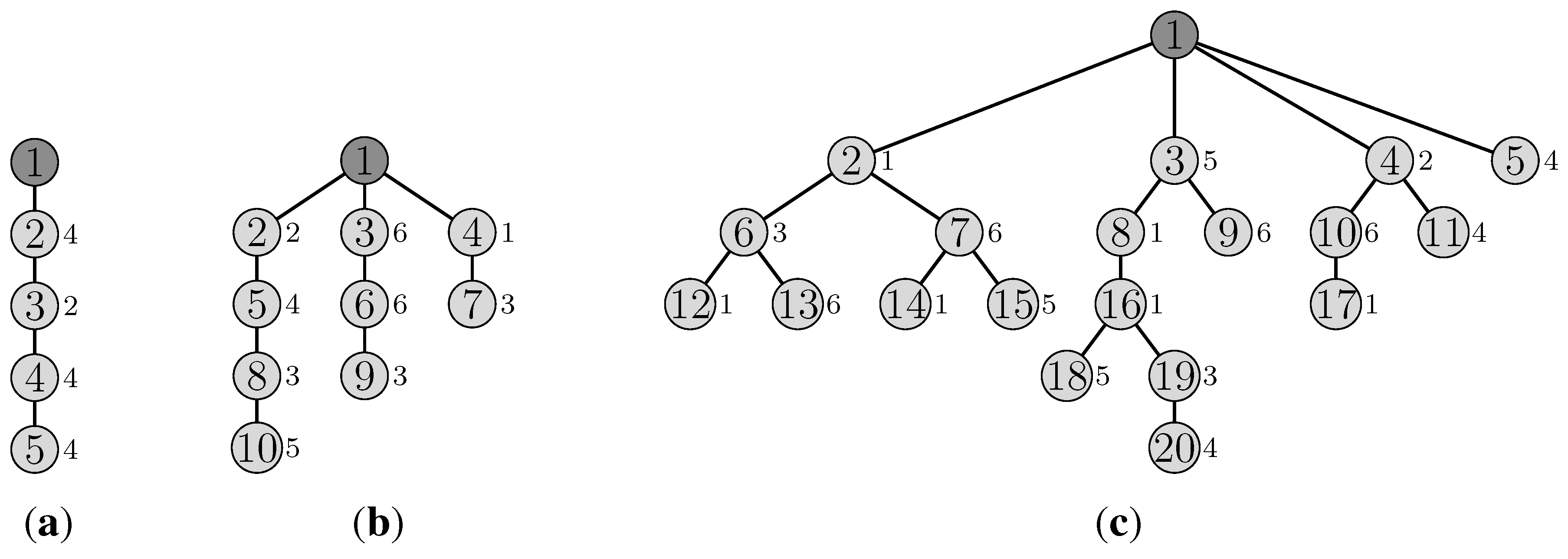
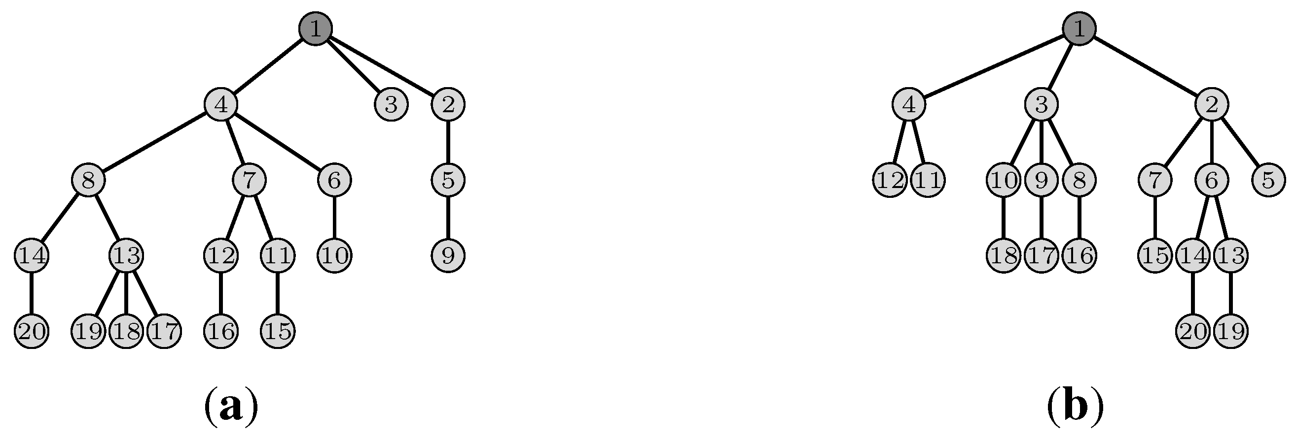
extra slots for the first bonus slot requested. For instance, in
Figure 4, a node at
will require six extra slots (see the grey slot path). For the next bonus slots required by
u, if any, each of them will require two extra slots (see the black slot path in
Figure 4 ending at slot 8). Indeed, the next transmission of
u cannot be scheduled in the next slot, where the parent of
u is transmitting. Similarly, all the bonus slots requested by the other nodes will need two additional extra slots. Hence, we get
extra slots. We can also notice that in the slot, where
u is scheduled, a node,
v, of depth,
, can be scheduled simultaneously, but on another channel (assuming that the links in the convergecast tree are the only topology links). Applying this property recursively, we can then schedule in the
first slots, one bonus request by a node of depth,
k, with
k varying from
to two if
is even and from
to one, otherwise. Hence, we finally get the maximum number of extra slots equal to
, with:
| = | | if is even, |
| | = | | otherwise, |
■
Notice that this bound does not take into account the possible parallelism between simultaneous transmissions of nodes belonging to the same depth. AMSA takes advantage of this parallelism.
Figure 4.
Extra slots scheduling when .
Figure 4.
Extra slots scheduling when .
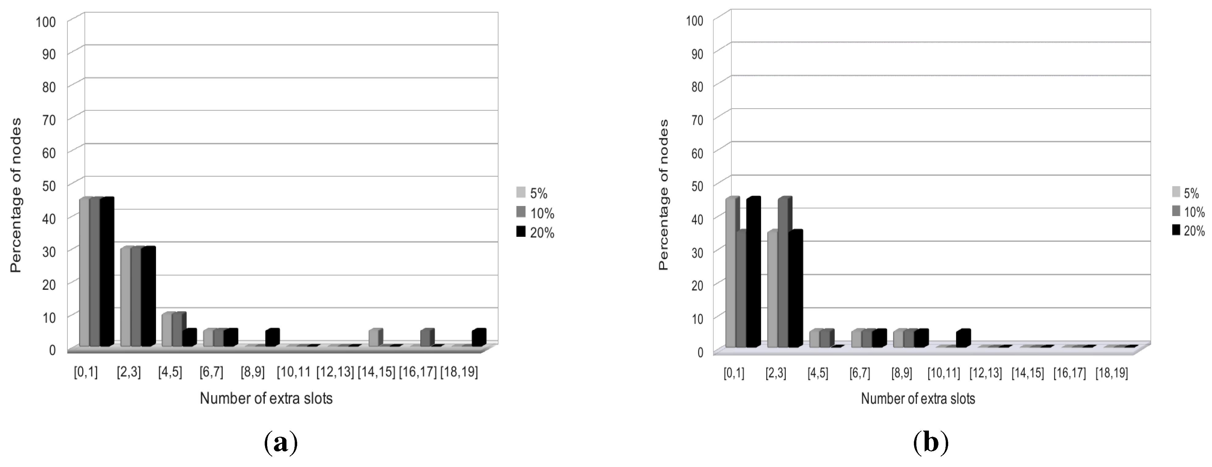
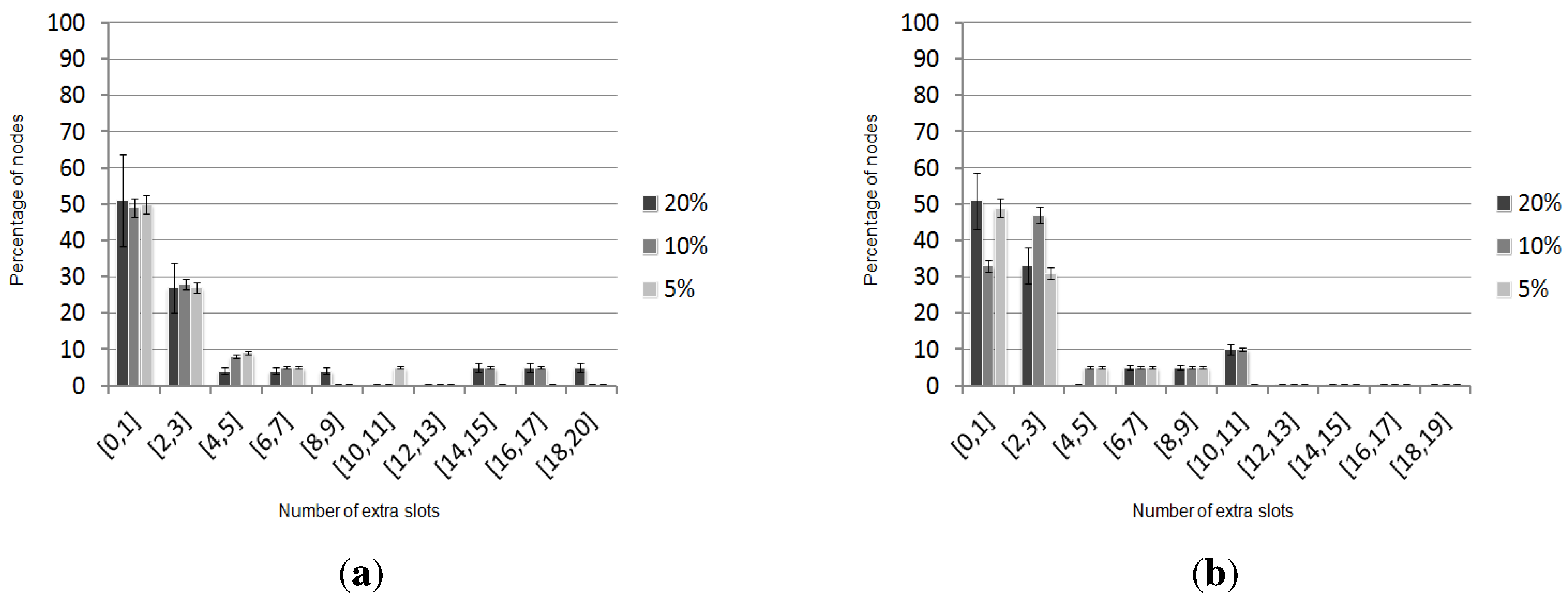
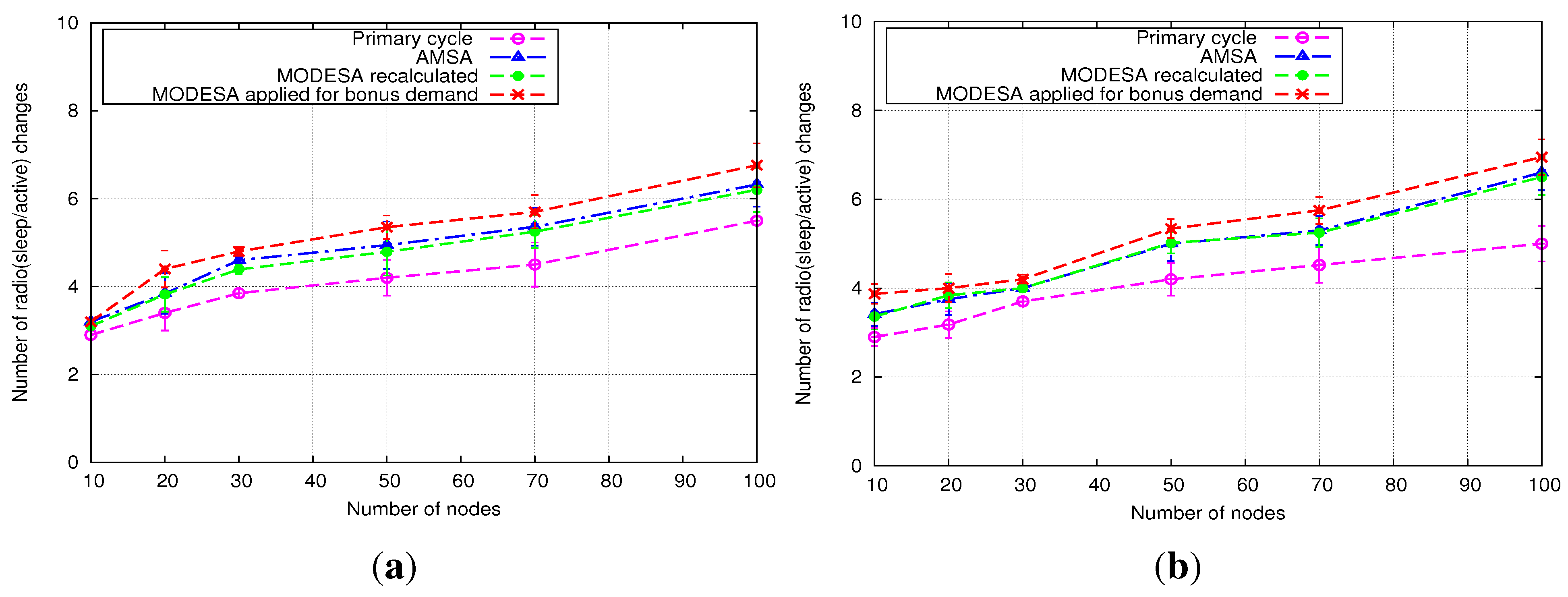
The performance evaluation reported in
Section 5 will show how AMSA is close to the lower and upper bounds. We will also position AMSA with regard to an intermediate solution, where an optimized time slot assignment is computed by MODESA from the bonus slots requests and appended at the end of the primary schedule.
4.6. Illustrative Example
In this section, we provide two scenarios of bonus slot assignment.
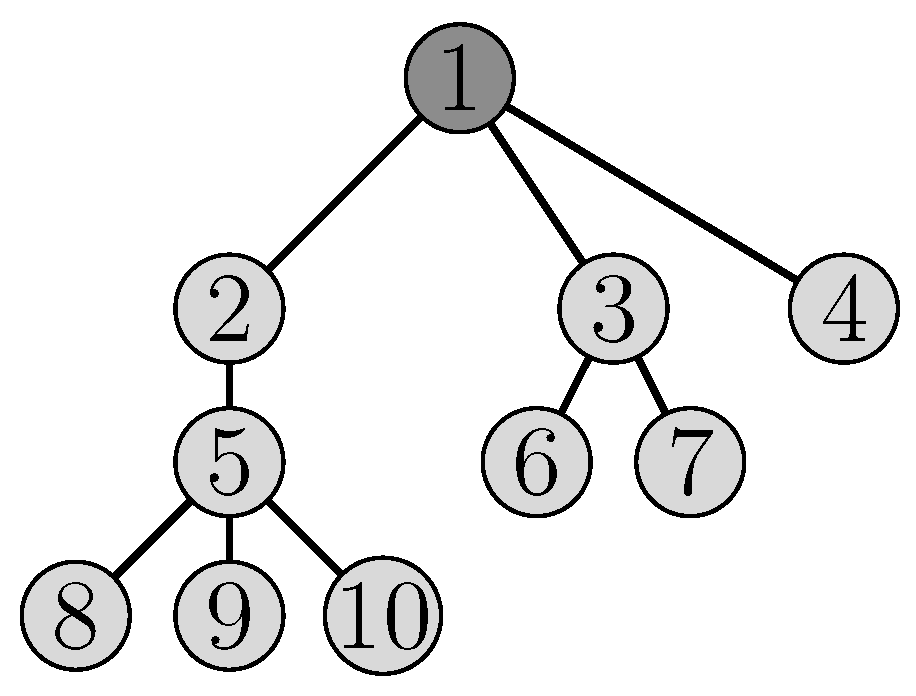
Figure 5 presents the topology of the network studied in our example. This network is composed of 10 nodes, including the sink (node 1). The sink has two radio interfaces. In both scenarios, there are two channels available at each node.
Figure 5.
The topology of the network.
Figure 5.
The topology of the network.
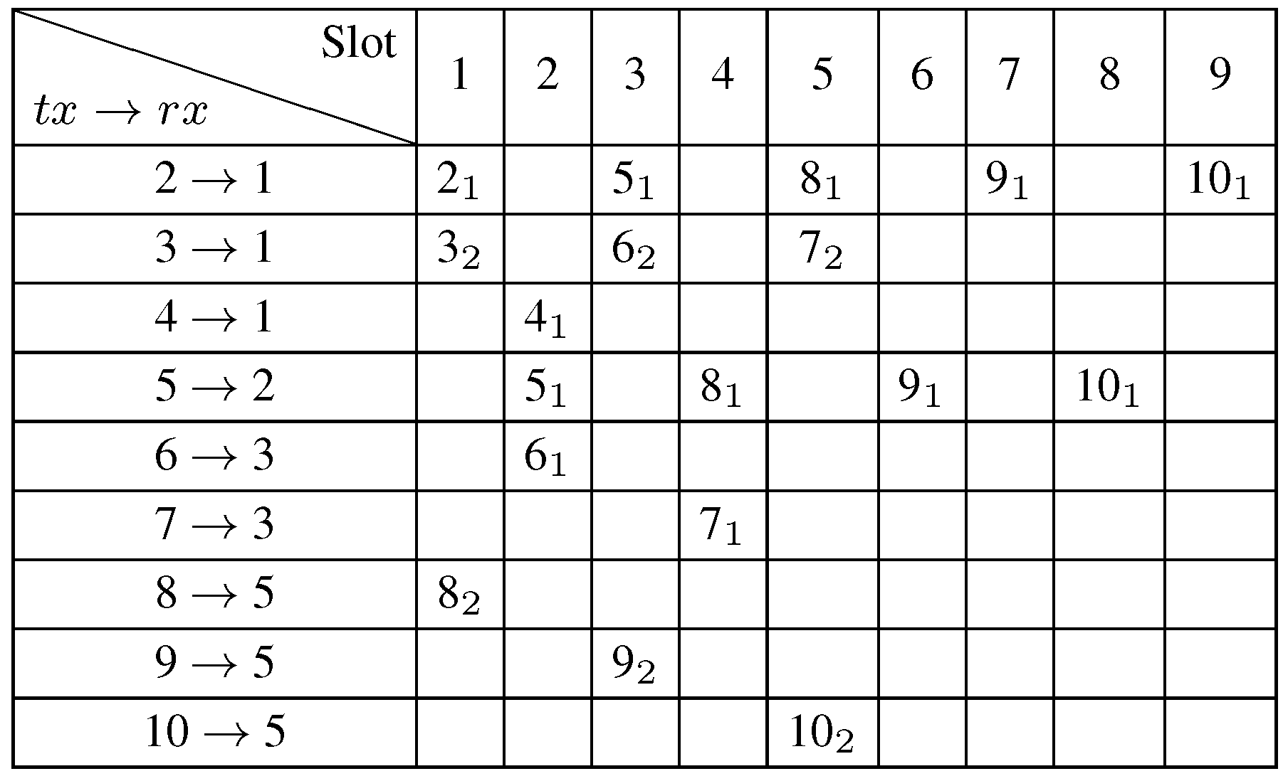
The optimal primary schedule given by MODESA is depicted in
Figure 6. This assignment has a length of nine slots and corresponds to a primary demand of only one packet generated at each node except the sink. Slots are represented by a column. The notation,
, means that node 2 transmits data to its parent on channel 1.
Figure 6.
The primary schedule.
Figure 6.
The primary schedule.
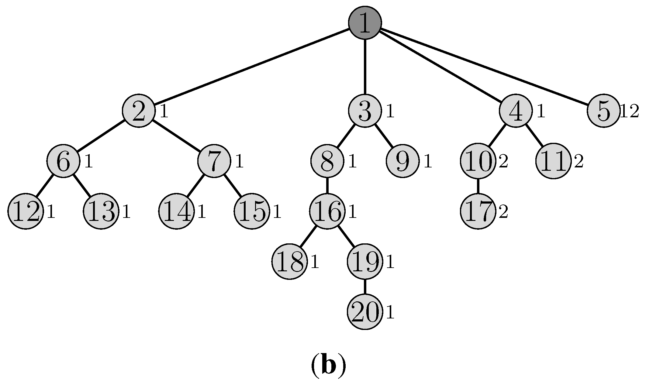
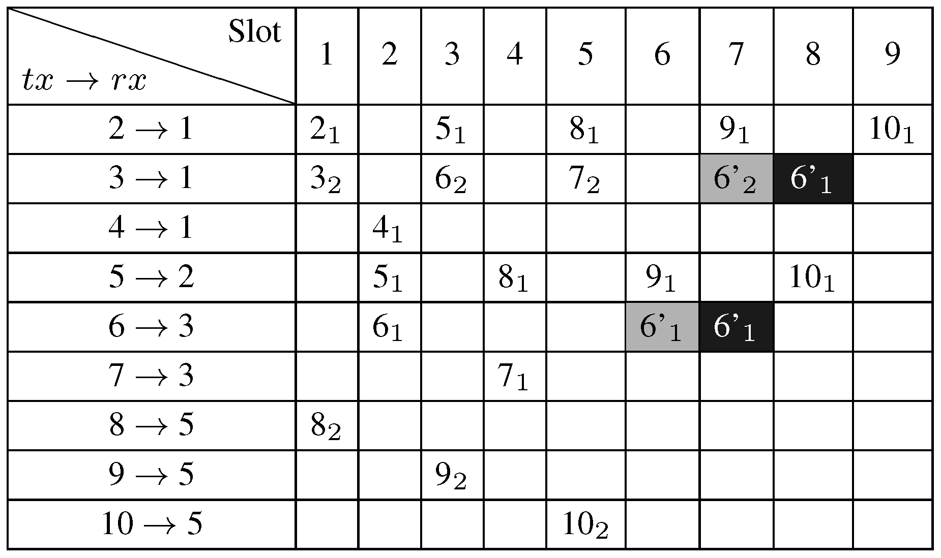
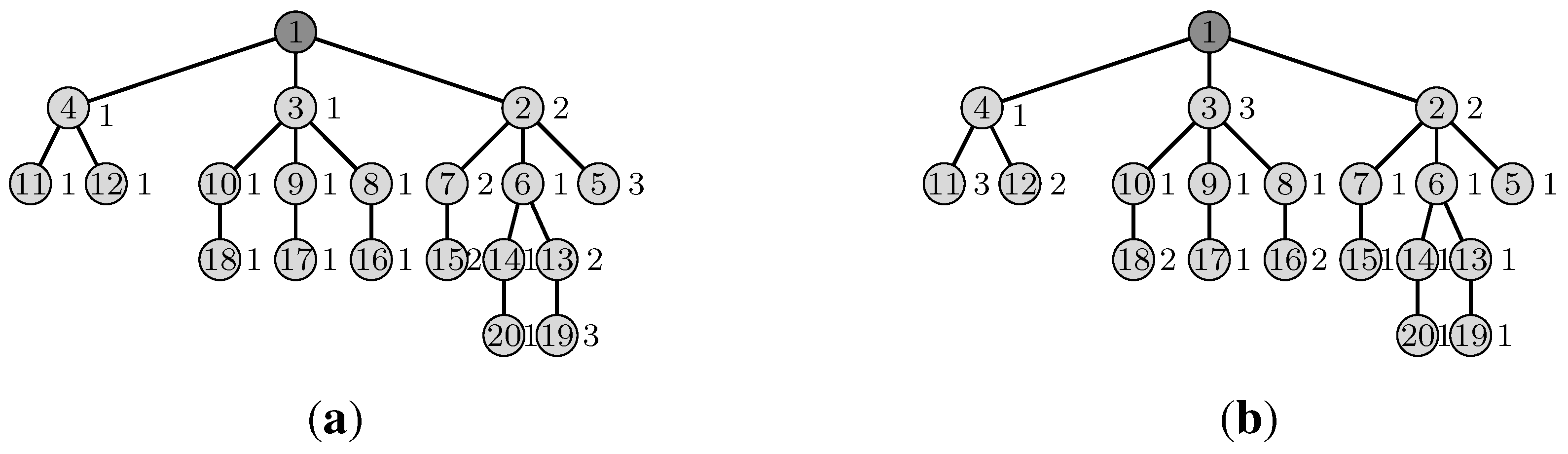
Figure 7 shows the primary schedule with the bonus slot assignment for the bonus request of node 6 asking for an additional slot. These results are given by the GLPK linear program (in black cells) and by the AMSA algorithm (in grey cells), respectively. In this scenario, we observe that the schedule length is unchanged, despite the bonus path assignment from node 6. This is due to the available spatial reuse.
Figure 7.
The bonus slot assignment for node 6.
Figure 7.
The bonus slot assignment for node 6.
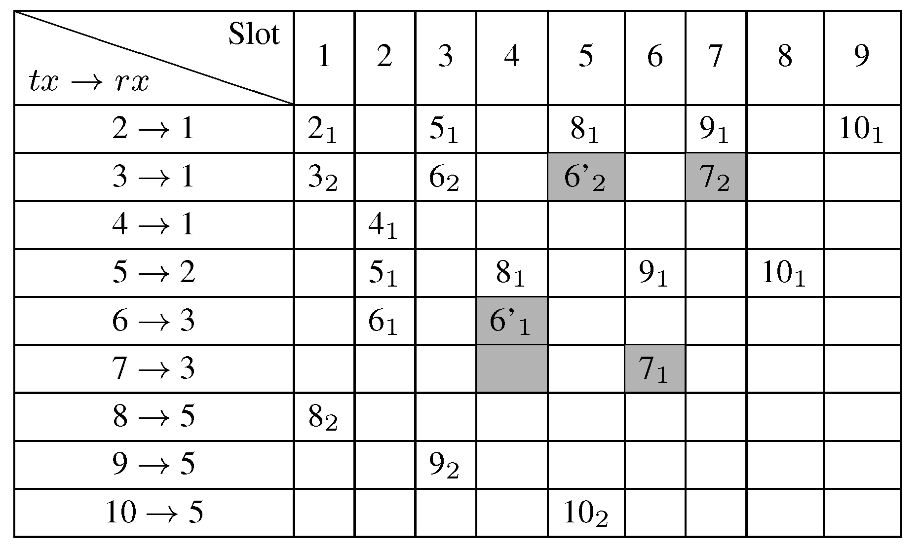
The new optimal slot assignment given by MODESA that takes into account the additional demand of node 6 is presented in
Figure 8. Changes from the primary schedule are represented in grey. Since this schedule is optimal and has the same length as the schedule modified by AMSA, the solution we propose, it follows that there exist scenarios where AMSA provides the optimal solution.
Figure 8.
The new slot assignment taking into account the additional demand of node 6.
Figure 8.
The new slot assignment taking into account the additional demand of node 6.
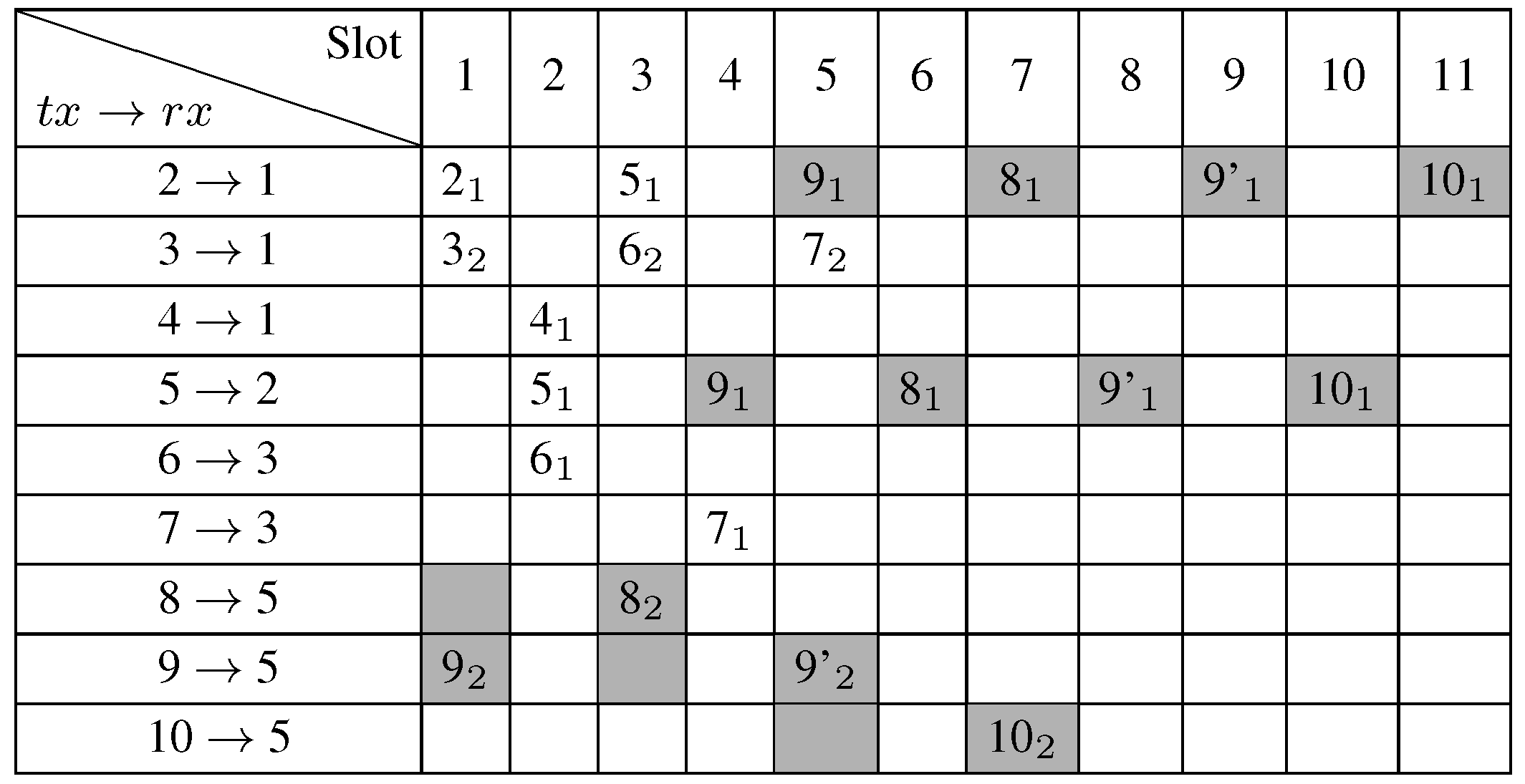
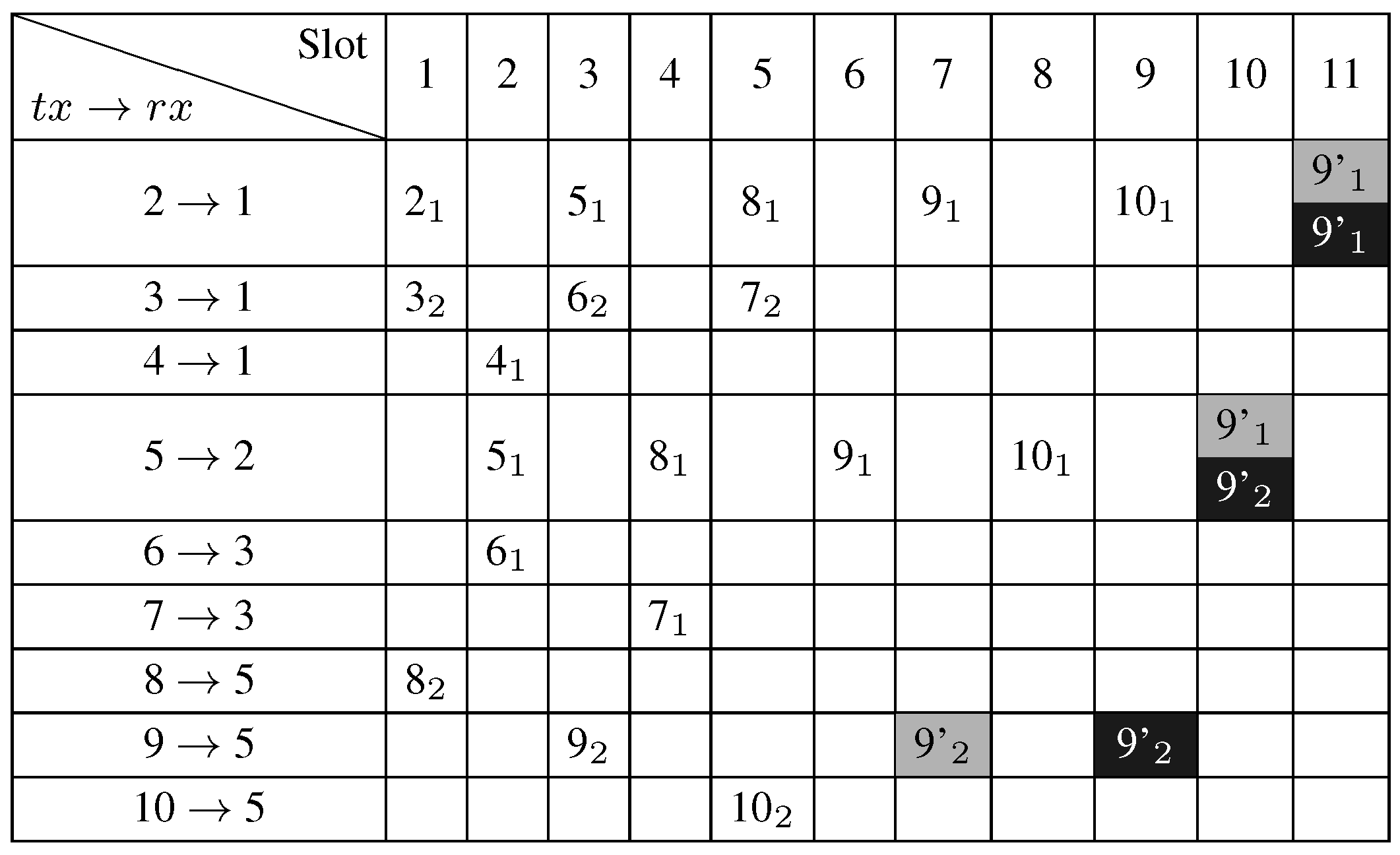
Figure 9 describes the bonus slot assignment for the bonus request of node 9 asking for an additional slot. In this case, the bonus slot assignment overflows from the primary schedule, taking slots from the inactivity period (slots 10 and 11).
Figure 9.
The bonus slot assignment for node 9.
Figure 9.
The bonus slot assignment for node 9.
With the additional demand of node 9, MODESA obtains the assignment presented in
Figure 10.
In both examples, AMSA obtains the same schedule length as the linear program; so its bonus slot assignment is optimal for these scenarios. Moreover, the bonus slot assignment has the same number of slots as with a complete recomputation of the optimal assignment obtained with the GLPK model presented in Section [
2], taking into account the initial and additional transmission needs. We can also deduce from these examples that the length of the new schedule depends not only on the additional bonus slots requested, but also on the depth of requesting nodes in the convergecast tree.
Figure 10.
The new schedule taking into account the additional demand of node 9.
Figure 10.
The new schedule taking into account the additional demand of node 9.


