1. Introduction
By the advances of the Micro Electro Mechanical Systems (MEMS) and communication theory, wireless networking and embedded processing, ad-hoc networks of devices and sensors capabilities are becoming increasingly available for commercial applications such as environmental monitoring (e.g., traffic, habitat, security), industrial sensing (e.g., factory, appliances), and critical infrastructure protection applications (e.g., power grids, water distribution, waste disposal). For these purposes, each sensor node collaborates with others in sensing, monitoring, and tracking events of interests by exchanging acquired data, usually stamped with the time and position information. In many of these applications, knowledge about sensors’ geometrical positions are critical for many network protocols, e.g., topology control, geographical routing, and clustering [
1]. It thus becomes one of the fundamental issues in Wireless Sensor Networks (WSNs) to acquire sensor position knowledge, called sensor localization problem.
In WSNs, positioning errors can often be masked by features such as fault tolerance, node redundancy, data aggregation and other means [
2,
3]. This makes coarse accuracy of sensor localization sufficient for many WSNs applications. Range-free localization is therefore pursued as a cost effective alternative for expensive range based scheme, by having no dependence on the availability or validity of hardware to provide range information. The key idea is to place a small fraction of anchors (
i.e., special sensors with known positions) across the network. Positioning of sensors is obtained from the estimated distance to multiple anchors and their coordinates, according to trilateral algorithm.
Previous range-free localization work mainly focuses on regular sensor deployment areas [
4],
i.e., sensors are uniformly and densely distributed in a convex region. However, this assumption does not hold when a sensor network is deployed in irregular areas with obstacles, because the packet delivery path between two sensors can be detoured by obstacles and this shortest path distance is dramatically different from its geographical Euclidean distance. These detoured obstacles are inevitable in natural areas such as valleys where sensors are deployed for habitat monitoring, as well as in urban areas where sensors can be separated by buildings. Therefore, when applying range-free techniques to the concave areas, the position estimates may in fact contain large errors [
5]. One response to this irregular area problem is to partially ignore the erroneous distance information by using an improved multi-hop algorithm [
6]. Yet, distorted anchor information can mislead accurate position estimates. One way to improve the accuracy of localization would be to rule out distorted path information from some anchors, which however has two particular difficulties. First, because sensors do not have the global view of their network, they have no way of determining which path information is distorted and which is not. Second, anchors can rely on the information that they receive from other anchors that are in an unobstructed straight line path, because they are able to determine their mutual reliability based on the calculation of an expected hop length. However, anchors and sensors cannot rely on each other in this way because sensors do not know their own locations and so cannot make an expected hop-length calculation.
In this paper we introduce a novel method based on angular information of the detour transmission path to estimate the optimal path distance between any pair of sensor nodes in WSNs with arbitrary node density and low anchor to sensor ratio. The proposed algorithm leads to a good position determination for WSNs as compared with some existing positioning schemes such as pattern-driven [
7], DV-Hop [
8], Gang
et al. [
9], Chen
et al. [
10] and Hop-Count-based Neighbor Parition (HCNP) [
11]. The main contributions of this paper are as follows:
The average localization error is approximately less than 0.3r (r is the radio range of sensors) and 0.35r in isotropic and anisotropic network respectively. This localization accuracy can satisfy the needs of many location-dependent protocols and applications, including geographical routing and tracking [
2]. Compared with previous localization algorithms that declares to tolerate network anisotropy, our localization scheme excels in (1) higher accuracy stemming from its ability to tolerate multiple anisotropic factors, including the existence of obstacles, sparse sensor distribution, and anisotropic terrain condition; (2) localization accuracy guaranteed by theoretical analysis and simulation results; and (3) a distributed solution with comparative communication overhead but high accuracy and enhanced robustness to different network topologies and different degree of irregualrities.
The rest of the paper is organized as follows. We start by related work in
Section 2.
Section 3 describes the network model. Our proposed algorithm is presented in
Section 4. In
Section 5, simulation results are shown and localization performances are discussed. Finally, we present our conclusions in
Section 6.
2. Related Work
Many range-free approaches have been proposed to determine sensor locations in WSNs. For example, the Centroid method [
12] is probably the earliest and simplest range-free approach, in which each node estimates its location by calculating the center of all the anchors it hears. APIT [
2] lets each node estimate whether it resides inside or outside several triangular regions bounded by the anchors it hears, and refines the computed location by overlapping the regions a sensor could possibly reside in. In order to improve accuracy, APIT needs many anchors and assumes that the anchors have radio ranges that are 10 times larger than those of ordinary nodes. Another proposed space embedding approach [
13] rely on Multidimensional Scaling (MDS) or Singular Value Decomposition (SVD) based techniques to project the node proximities into geographic distances.
DV-Hop employs a constant number of anchors and relies on the heuristic of proportionality between the distance and hop count in isotropic networks. The system estimates the average distance per hop from anchor locations and the hop count among anchors. Each node measures the hop count to at least three anchors and translates these into distances. By triangulation, the location is then calculated. However, the DV-Hop method yields high localization errors in anisotropic networks, where the existence of holes breaks the proportionality between the distance and hop count and thus leads to inaccurate location estimates.
To modify the disadvantage of existing DV-Hop localization algorithm, the relevant literature proposed many improved algorithms [
9,
10,
14,
15]. In [
9], the location accuracy is improved bymodifying the network average hop distance based on minimum mean square error criteria as
![Jsan 02 00025 i001]()
, where
dij is the straight line distance between the anchor node
i and
j,
hj is the hop segment number between the anchor nodes
i and
j. Another algorithm in [
10] calculates the error
eij as
![Jsan 02 00025 i002]()
, where
![Jsan 02 00025 i003]()
is the estimated distance between anchor nodes
i and
j,
![Jsan 02 00025 i004]()
is is the Euclidean distance between anchor
i and
j. The average hop distance is finally adjusted by
![Jsan 02 00025 i005]()
where
m is the closest anchor node to anchor node
i and
HopSizei is calculated as
![Jsan 02 00025 i006]()
where (
xi,
yi) (
xj,
yj) are the coordinates of anchor node
iand
j and
hij is the number of hops between anchor
iand
j. The Algorithms [9,10] made improvements on distance estimation and localization of the DV-Hop algorithm. There are still some disadvantages in the improved algorithms, such as no obvious improvement on localization accuracy, especially when the transmission route is not straight but detoured.
Another pattern driven localization scheme is proposed in [
7] to tolerate network anisotropy. The paper proposes three different methods of anchor-sensor distance calculation based on three patterns, namely Concentric Ring (CR): isotropic pattern, Centrifugal Gradient (CG): anisotropic but slightly detoured, and Distorted Gradient (DG): anisotropic and strongly detoured. For the CR pattern, it utilizes the last hop distance for overall distance calculation. The method is based on the neighbor node degree of a sensor node. It requires high node density to work properly. For the CG pattern, the author proposes DiffTriangle to revise the anchor-sensor distance estimates with the assistance from the nearest anchor to the sensor (namely Reference Station), which exhibits the CR pattern. This implies that these reference stations should appear in normal sensors’ CR category and thus the distance from sensors to their dominating reference stations should be no more than three or four hops. This assumption implicitly places a high demand for anchor distribution density. In DG pattern, the anchors which falls in DG category are dropped and no longer be used for location estimation. However it may be impossible in practice to accurately recognize the slightly detoured anchors from the strongly detoured anchors or even moderately detoured anchors, without the global knowledge on network topology,
i.e., network boundary and obstacles shapes.
In the REndered Path (REP) algorithm [
16], the authors assumed that the boundaries of holes in the network have been detected and every node knows if it is a boundary node or not. The authors proposed an approach for computing the straight line distance between two nodes by arguing corresponding shortest path with virtual holes. In HCNP [
11], the author proposed source to destination distance estimation algorithm based on the observation that the neighbors of a destination can have different hop counts with respect to the same source and such information is used to improve the localization accuracy only in isotropic network.
3. Network Model
When sensor nodes are randomly deployed in WSNs, we cannot assume any regularity in spacing or pattern of the sensors. This is due to the fact that most of the cases sensors are deployed from the low flying airplanes or unmanned ground vehicles. However anchors can be placed randomly or in the form of regular tile across the network so as to help in estimating the sensors positions [
17]. In this paper we place anchor and sensor nodes randomly, which is more practical.
Consider a WSNs in a 2D plane with
N sensors, denoted by a set
![Jsan 02 00025 i007]()
where
si is the
ith sensor node. All sensor nodes are uniformly and independently deployed in a square area
A =
L×
L. Such a random deployment results in a 2D Poisson distribution of sensors with sensor density
![Jsan 02 00025 i008]()
. All sensors are assumed to be homogeneous and stationary and omnidirectional. Therefore the network can be seen as static or regarded as a snapshot of mobile ad hoc sensor networks. In order to simplify the discussion, we are not concerned with the issues of energy consumption and robustness of sensor nodes. We believe that these missing issues do not invalidate the correctness of the proposed method.
Definition 1: Let a (si,r) define the transmission range or radio coverage area of a sensor si ,where the center is sensor si and the transmission radius is r. The radio coverage area of any sensor is assumed to be circular and symmetrical. So a (si,r) = πr2. Any sensor nodes that are located within this area can directly communicate with each other and is defined as neighbors of each other. It is because we assume that all the sensors have the same transmission capability.
Definition 2: Let
NE be the average number of sensors located in the radio coverage area. The average connectivity denoted by
CE is defined as the average number of neighbor sensors located in the sensors transmission range. Following definition 1, the transmission coverage area is
a (
si,
r) =
πr2. The sensor density of the network is
![Jsan 02 00025 i008]()
. Therefore
NE =
λπr2 and
CE =
NE − 1.
4. The Proposed Algorithm (DPAI)
In real life scenarios, the sensor nodes are deployed randomly from the airplanes in areas where obstacles or holes may exist. Because of obstacles or holes, the packet transmission paths among anchor and sensor nodes are not always straight but detoured. In range-free localization, the exact hop distance calculation is the key problem for estimating location. The average hop distance of the network heavily depends on the data transmission path, i.e., if the transmission path is almost straight, then the average hop distance is almost accurate, otherwise deviated from its actual value if there is an obstacle in between. We observe that, if we can associate the angle of the detoured transmission path with the calculation of the average hop distance, then we can accurately calculate the average hop distance and hence the localization. Utilizing this concept of angular information of the detoured transmission path, we propose the DPAI algorithm for precise localization.
4.1. Detour Path Angular Information Based Localization
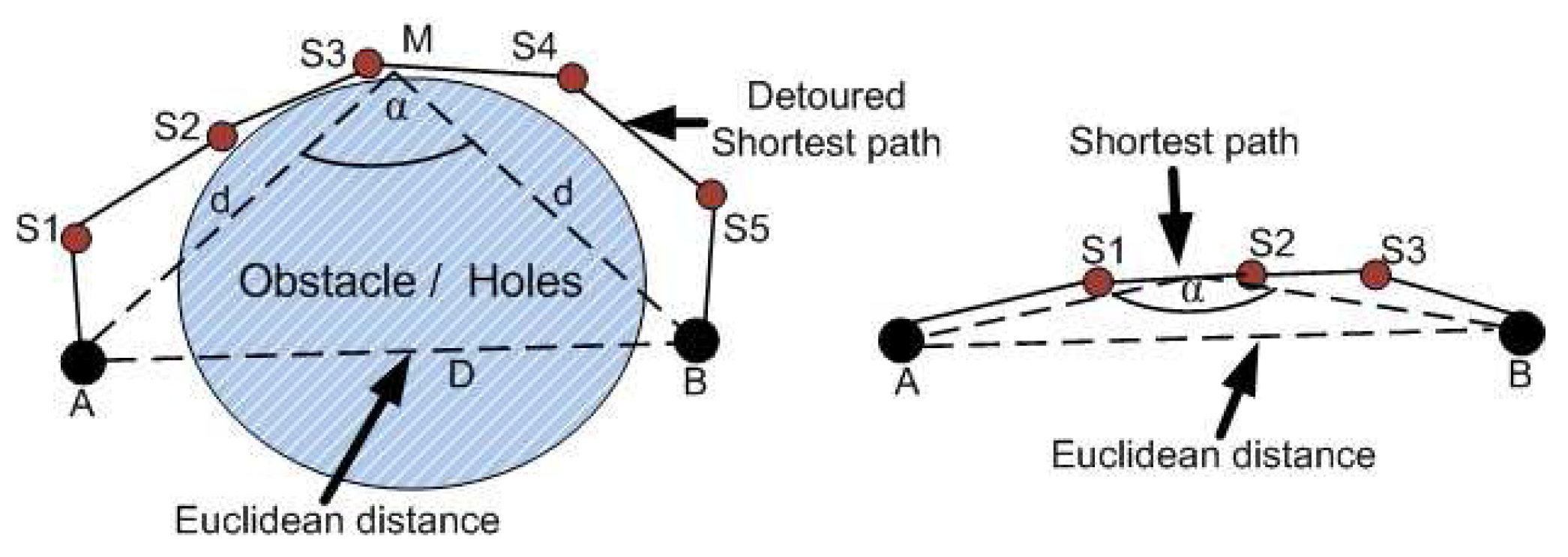
Suppose that two anchor nodes A and B are separated by an obstacle and thus connected by a detoured shortest transmission path
A –
S1 –
S2 –
S3 –
S4 –
S5 –
B as shown in
Figure 1 (left hand side). From the figure, we can see that the angle
α between the two anchors and the middle of the shortest transmission path is closely related to the length of the transmission path. The angle approaches to 180° if the transmission path is almost straight (
A –
S1 –
S2 –
S3 –
B) as shown in
Figure 1 (right hand side), otherwise the angle is much smaller as shown in
Figure 1 (left hand side). Suppose the Euclidean distance between anchor nodes
A and
B is
D, the distance from anchor
A and
B to the middle of the transmission path is
dand the number of hop between these anchor nodes is
Nh.
Figure 1.
Packet transmission path between two anchors with obstacle and without obstacle.
Figure 1.
Packet transmission path between two anchors with obstacle and without obstacle.
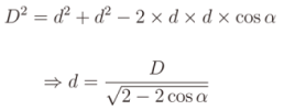
Now from ΔAMB , we can write,
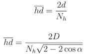
Therefore the average hop distance is
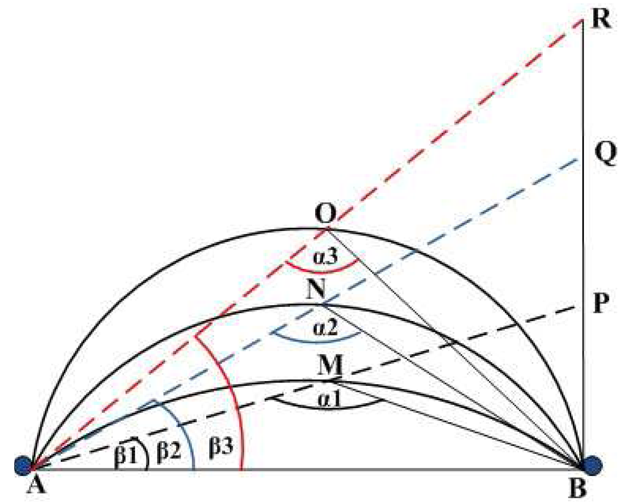
From
Figure 2 we can see the relation between transmission path length and the angle
α. There are three different transmission paths from anchor
A to anchor
B, namely transmission paths
AMB, ANB and
AOB respectively. Obviously the path lengths are different,
i.e.,
AMB <
ANB <
AOB. We draw the line
AP through the middle
M of the transmission path
AMB and draw one line from
P to
B in such a way that the triangle △
APB is right angle triangle, where ∠
ABP is the right angle. Similarly we draw the line
AQ and
AR. From every middle point of the transmission path we draw one line to
B. The lines are
MB,
NB and
OB. Thus the angles
α1,
α2 and
α3 denote the transmission paths route bend degree, when the transmission path lengths are
AMB,
ANB and
AOB respectively. The angles
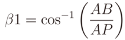
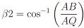
β1,
β2 and
β3 are defined as follows:
From the above equations, we notice that the value of
β is dependent on the length of transmission paths
AP,
AQ and
AR. This is because the path length
AB between two anchor nodes
A and
B, is constant for static sensor network. The longer the transmission paths, the larger the value of
β. Consequently the shorter the transmission path, the larger is the value of
α. In
Figure 2,
β3 >
β2 >
β1 and
α1 >
α2 >
α3. To calculate the value of α we present one example as follows:
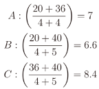
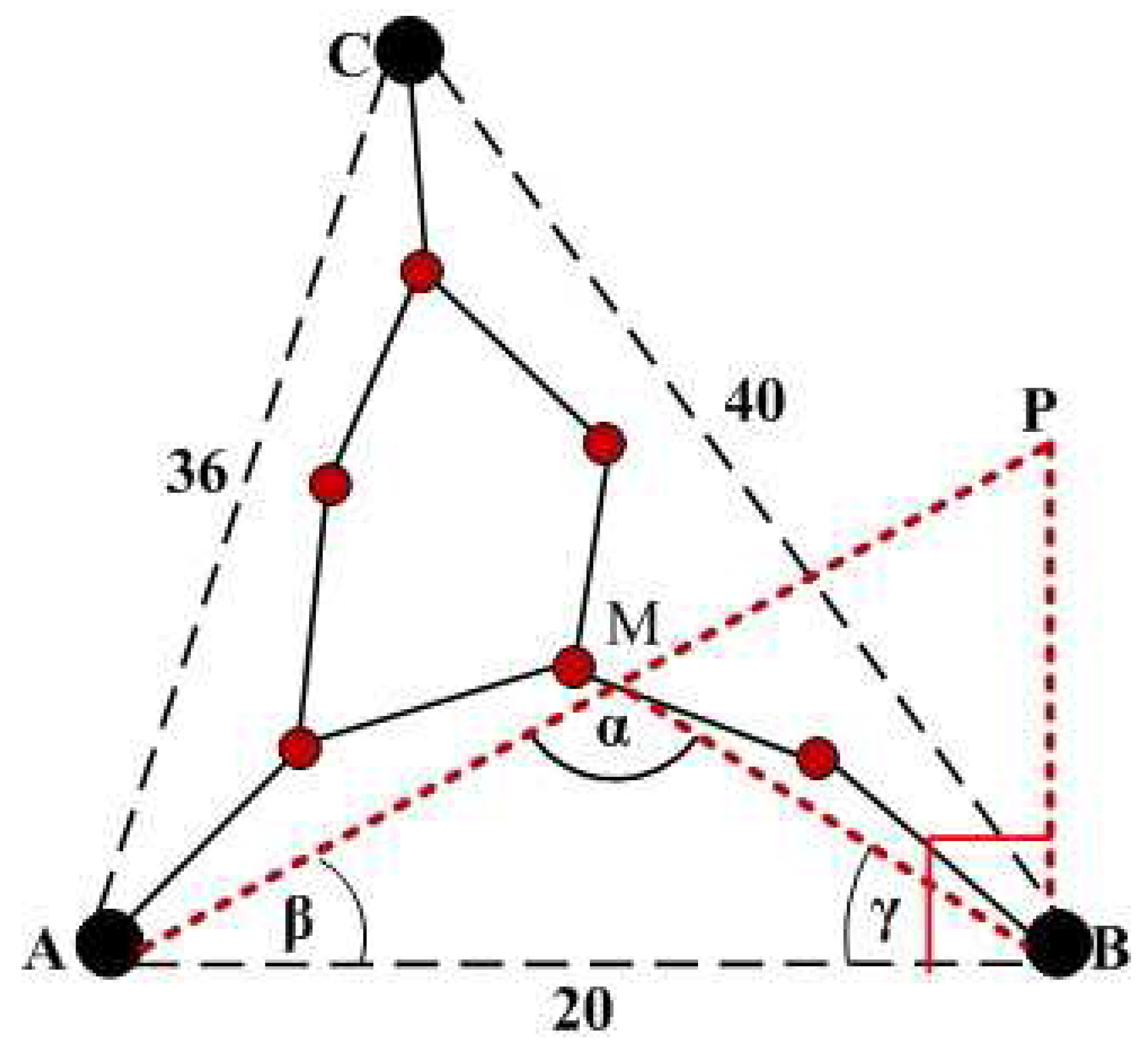
Suppose in
Figure 3,
A,
B and
C are three anchor nodes. The Euclidean distance between
A and
B is 20,
A and
C is 36 and
B and
C is 40 (the figure is not drawn to scale). Th number of hops between
A and
B is 4,
A and
C is 4 and
B and
C is 5. Each anchor node calculates the average hop distance as follows:
Now for simplicity, we can consider the case of anchor
A. After calculating the average hop distance,
A will calculate the Transmission Path Length (
TPL) by multiplying the number of hops and average hop distance. So from
A to
B, the
TPL is 4 × 7 = 28. But the Euclidean Distance(
ED) between
A and
B is 20, which is shorter than the
TPL. Since
TPL >
ED,
A assumes that the
TPL is detoured. To calculate the angle of the detoured transmission path, we draw one line
AP from
A to
P through the middle of the transmission path
M (Because the length of the transmission path is known) and whose length is the length of
TPL i.e., in our example 28. We draw one line from
P to
B in such a way that the angle ∠
ABP is right angle. From the middle
M, we draw another line to
B. From Δ
AMB, the two sides
AM and
BM are equal. Hence the angle
β =
γ. From Δ
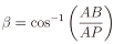
ABP, we know that,
The anchor node knows the value of
AB and
AP. So it can calculate the angle
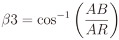
β. Now from Δ
AMB, we know that
In a similar manner, A can calculate the angle between A and C and accordingly adjust the average hop distance by (2). If TPL ≤ ED, then the value of β is set to 00 and accordingly, αcan be calculated by (7).
Figure 2.
Relation between transmission path length and the angle α.
Figure 2.
Relation between transmission path length and the angle α.
Figure 3.
Calculation of angle α.
Figure 3.
Calculation of angle α.
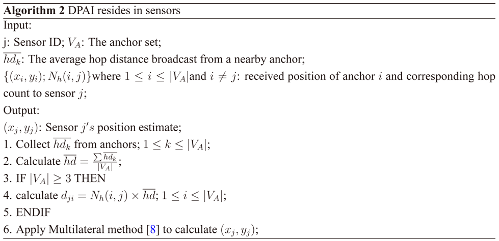
Algorithms 1 and 2 represent the pseudo codes of DPAI schemes. They represent the localization algorithms conducted in anchors and sensors respectively. VA represents the set of anchor nodes, TPLik represents the transmission path length and Dik represents the Euclidean distance between anchor i and k. At run time, similar to other range-free localization approaches such as DV-Hop, DPAI scheme ensures that anchor nodes first broadcast their locations and hop count value set to one. Each receiving node records the minimum hop count value from an anchor node and then flood outwards the same packet with hop count value incremented by one. Any packet containing larger hop count value than the previous one is ignored. Thus all nodes get the minimum hop number from every anchor nodes.
4.2. Analysis of Algorithm Complexity
Table 1 summarizes the protocol comparison of DPAI with DV-Hop and pattern-driven in various aspects including Communication Overhead (C.O), Computation Cost (C.C) and Applicable Network (A.N). To calculate the average hop distance, each anchor node needs 2 rounds of broadcasts. Consequently for an entire network the communication overhead is bounded by
O(
n2), where n is the total number of nodes in the network. The anchor nodes bear most of the computational burden. Each anchor node deals with angular information based average hop distance calculation and for each calculation, the anchor node does at most
O(
M) computations to calculate the average hop distance from the detour path, where
M is the number of holes or obstacles within the network. Thus for entire network each anchor’s computational overhead is
O(
nM).
Table 1.
Protocol Comparison.
Table 1.
Protocol Comparison.
| Protocol | C.O | C.C | A.N |
|---|
| DV-Hop | O(n2) | O(n) | Isotropic |
| pattern-driven | O(n2) | O(nM) | Isotropic,Anisotropic |
| DPAI | O(n2) | O(nM) | Isotropic,Anisotropic |
On the other hand, DV-Hop presumes isotropic network and triangulates the nodes location with its network distances to the three anchors. Each node floods the network for computing the hop count so the communication cost of DV-Hop is O(n2). Each anchor accepts requests from all the network and sends out feedback with O(n) computational cost. In the next section we will compare the localization accuracy of our approach through simulations.
5. Simulation Results and Performance Analysis
A series of simulations are conducted to evaluate the performance of our proposed scheme in isotropic and anisotropic WSNs, where anchor nodes are deployed randomly. For anisotropic network, we consider O-shape and C-shape network topology. For each of the different types of network, we run the simulation for 100 rounds and take the average over 100 runs, during which the quantity of the deployed sensor nodes is kept unchanged. However, the topology of the network varies because we establish connectivity between pair of sensor nodes randomly. To measure the accuracy of localization, the average localization error is used.
The average localization error is defined as the ratio of the differences between the estimated location
![Jsan 02 00025 i018]()
and the real location (
xi,
yi) to the communication range of sensor nodes. In this paper, the average localization error is expressed relative to the radio range r. The average localization error △ of the sensor network, which is composed of |
VS| sensor nodes, is expressed as follows:
The initial network parameters for simulations are shown in
Table 2. We vary the number of anchors and sensor density (the average number of sensors per sensor radio area) when necessary to observe their impact on localization errors.
Table 2.
Network Parameters for Simulation.
Table 2.
Network Parameters for Simulation.
| Network | For Isotropic | For Anisotropic |
| Parameter | Network | Network |
| Area | 10 × 10m | 10 × 10m |
| Sensor Nodes | 200 | 200 |
| Anchor Nodes | 20 | 20 |
| Radio Rnage | 2m | 2m |
For simulation, we compared our proposed algorithm with DV-Hop [
8], Gang
et al. [
9], Chen
et al. [
10], HCNP [
11] and pattern-driven [
7]. The results are shown in the
Figure 4 and
Figure 5 for isotropic network,
Figure 6 and
Figure 7 for O-shape, and
Figure 8 and
Figure 9 for C-Shape network. Also we investigate the impact of radio irregularity on the localization performance. The result is shown in
Figure 10. From the results, we can say that, our scheme has higher localization accuracy than HCNP [
11] (which cannot tolerate anisotropic factor) and pattern-driven [
7] (which can tolerate multiple anisotropic factor), DV-Hop [
8], Gang
et al. [
9], and Chen
et al. [
10]. Our scheme is robust in sparse isotropic network (
Figure 11), anisotropic (O-Shape (
Figure 12) and C-Shape (
Figure 13)) network, and under realistic system configurations where the radio transmission pattern of a sensor node varies per unit degree change in the direction of radio propagation as shown in
Figure 14 and
Figure 15. The other three methods degrades severely in anisotropic network and under different degree of radio irregularity. HCNP [
11], which is only designed for isotropic network, degrades severely in different anisotropic network conditions.
Figure 4.
Location error vs. number of anchor nodes (isotropic network).
Figure 4.
Location error vs. number of anchor nodes (isotropic network).
Figure 5.
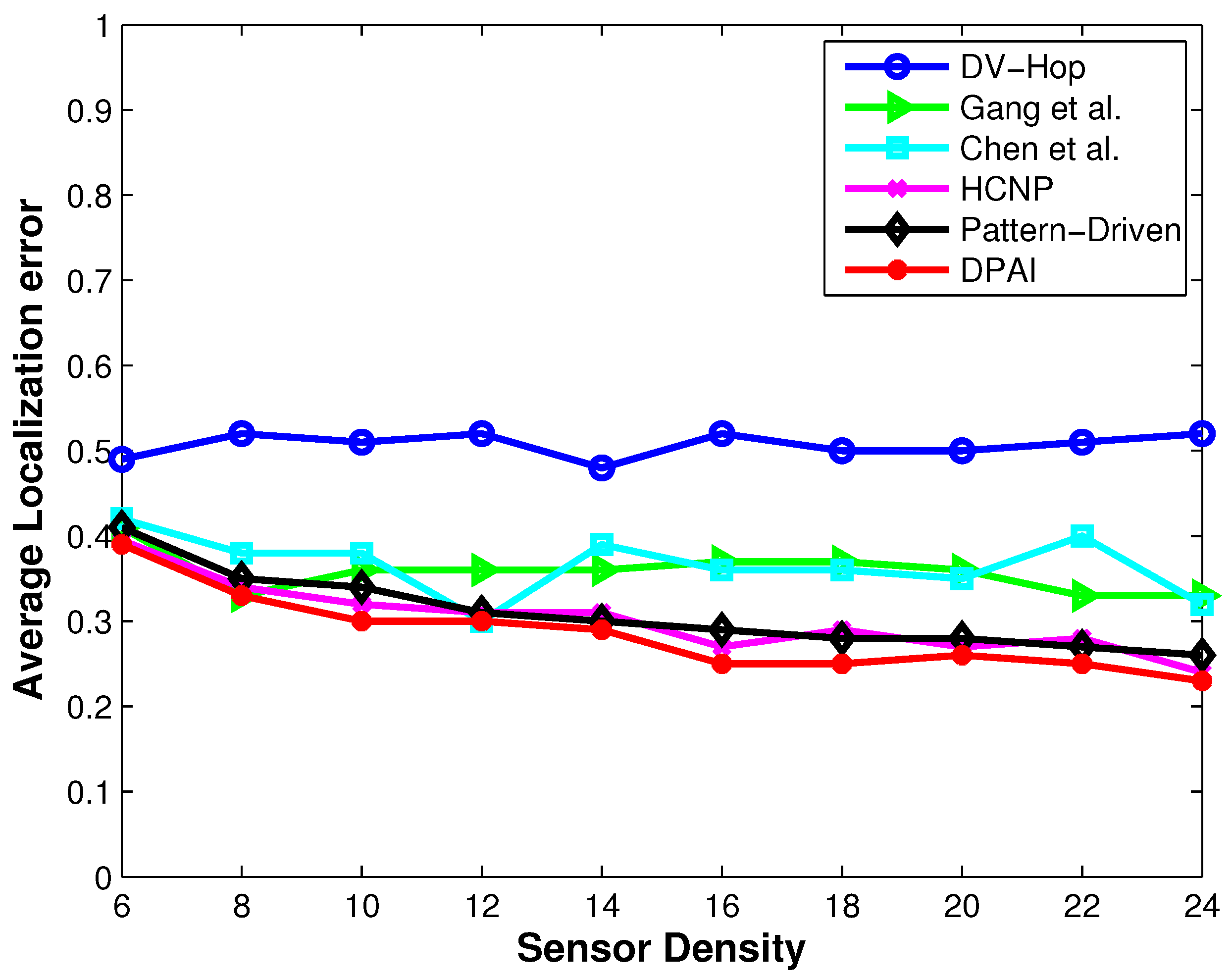
Localization error vs. sensor density (Isotropic network).
Figure 5.
Localization error vs. sensor density (Isotropic network).
Figure 6.
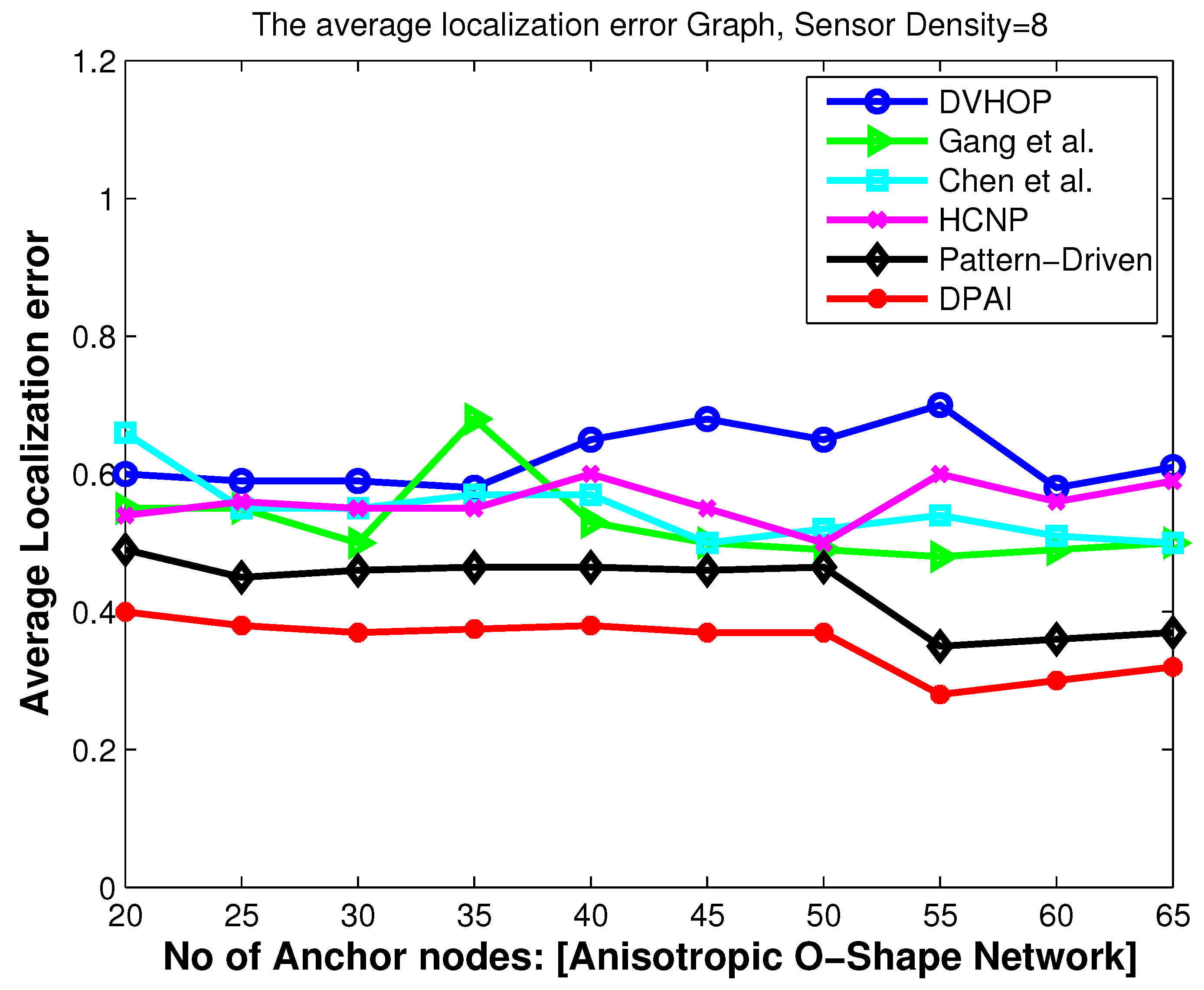
Location error vs. number of anchor nodes. (O-shape network).
Figure 6.
Location error vs. number of anchor nodes. (O-shape network).
Figure 7.
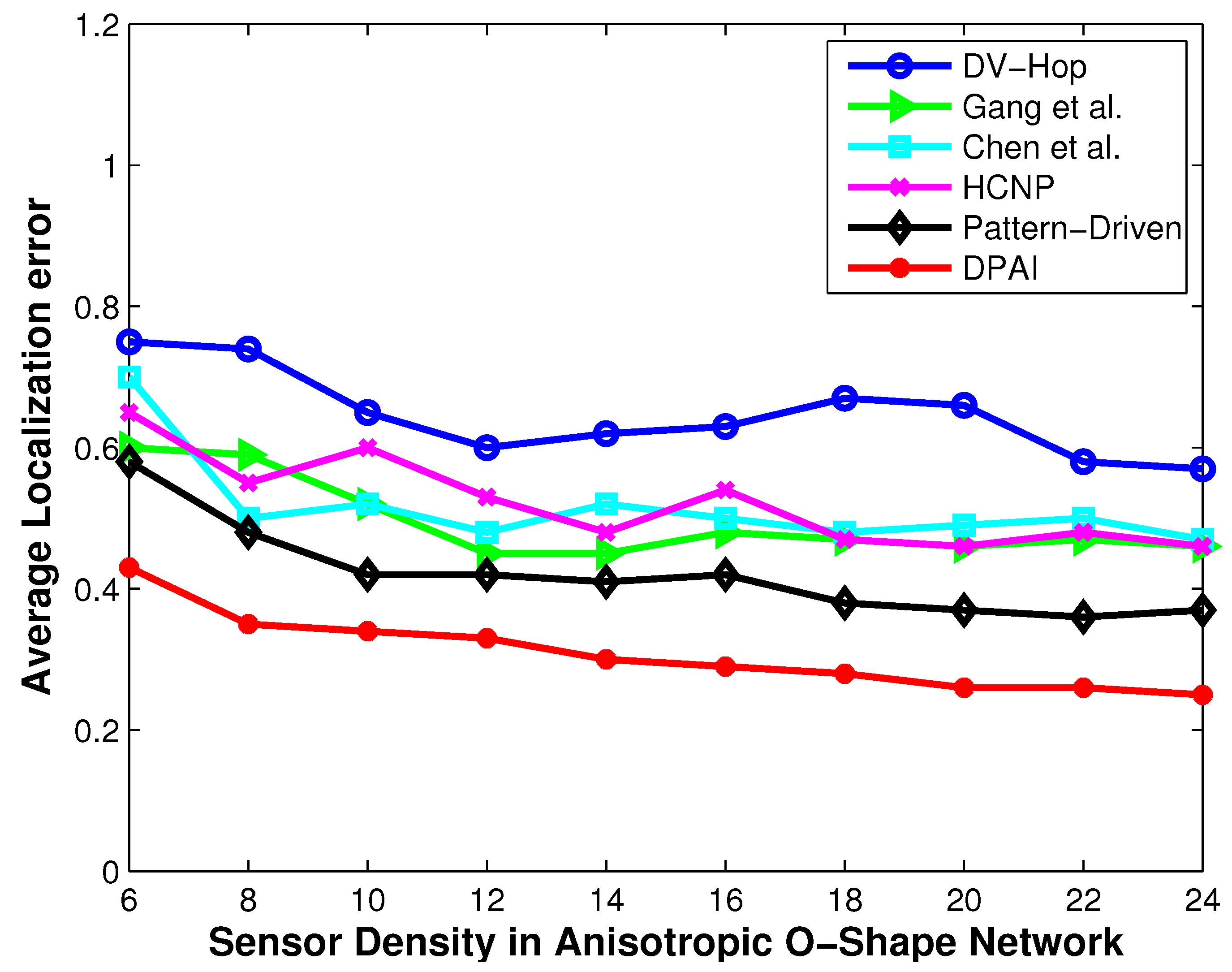
Localization error vs. sensor density (O-shape network).
Figure 7.
Localization error vs. sensor density (O-shape network).
Figure 8.
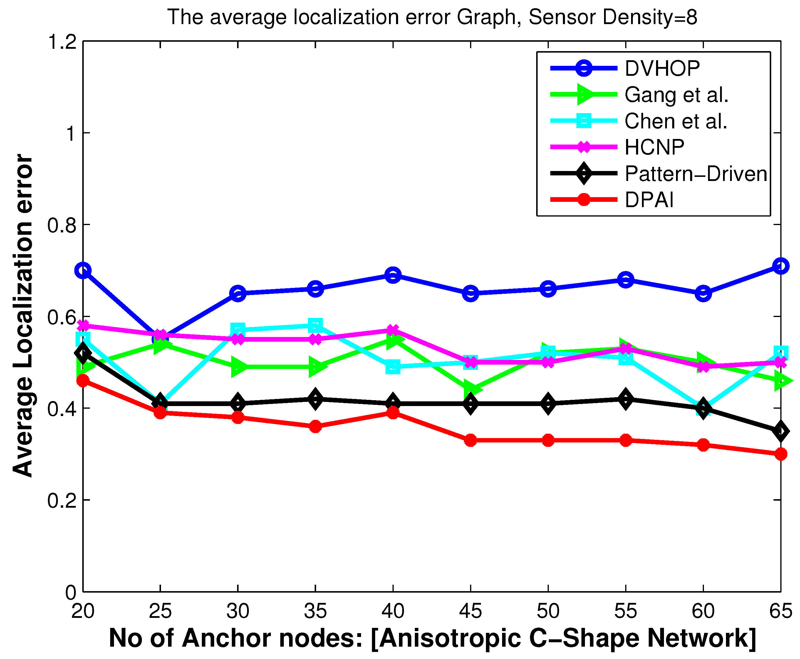
Location error vs. number of anchor nodes (C-shape network).
Figure 8.
Location error vs. number of anchor nodes (C-shape network).
Figure 9.
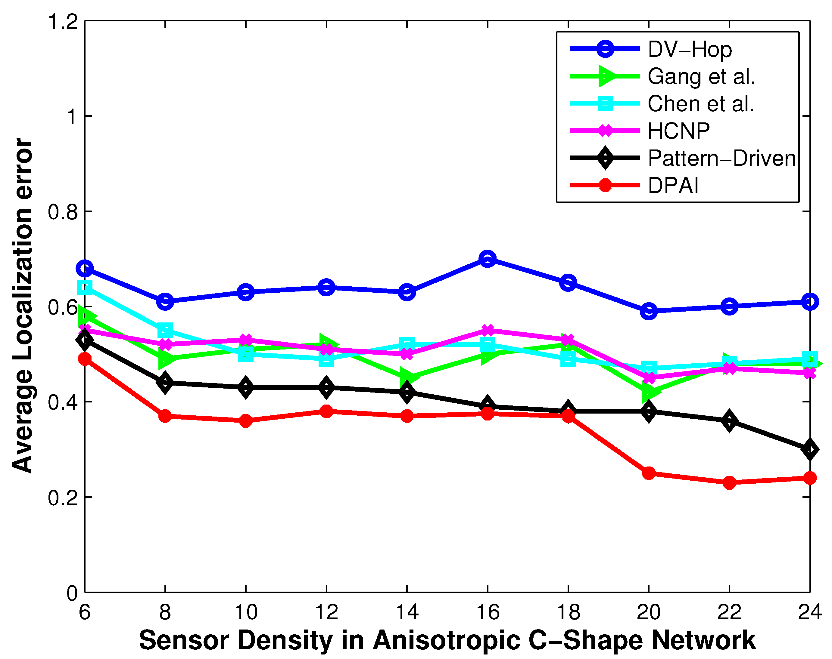
Localization error vs. sensor density (C-shape network).
Figure 9.
Localization error vs. sensor density (C-shape network).
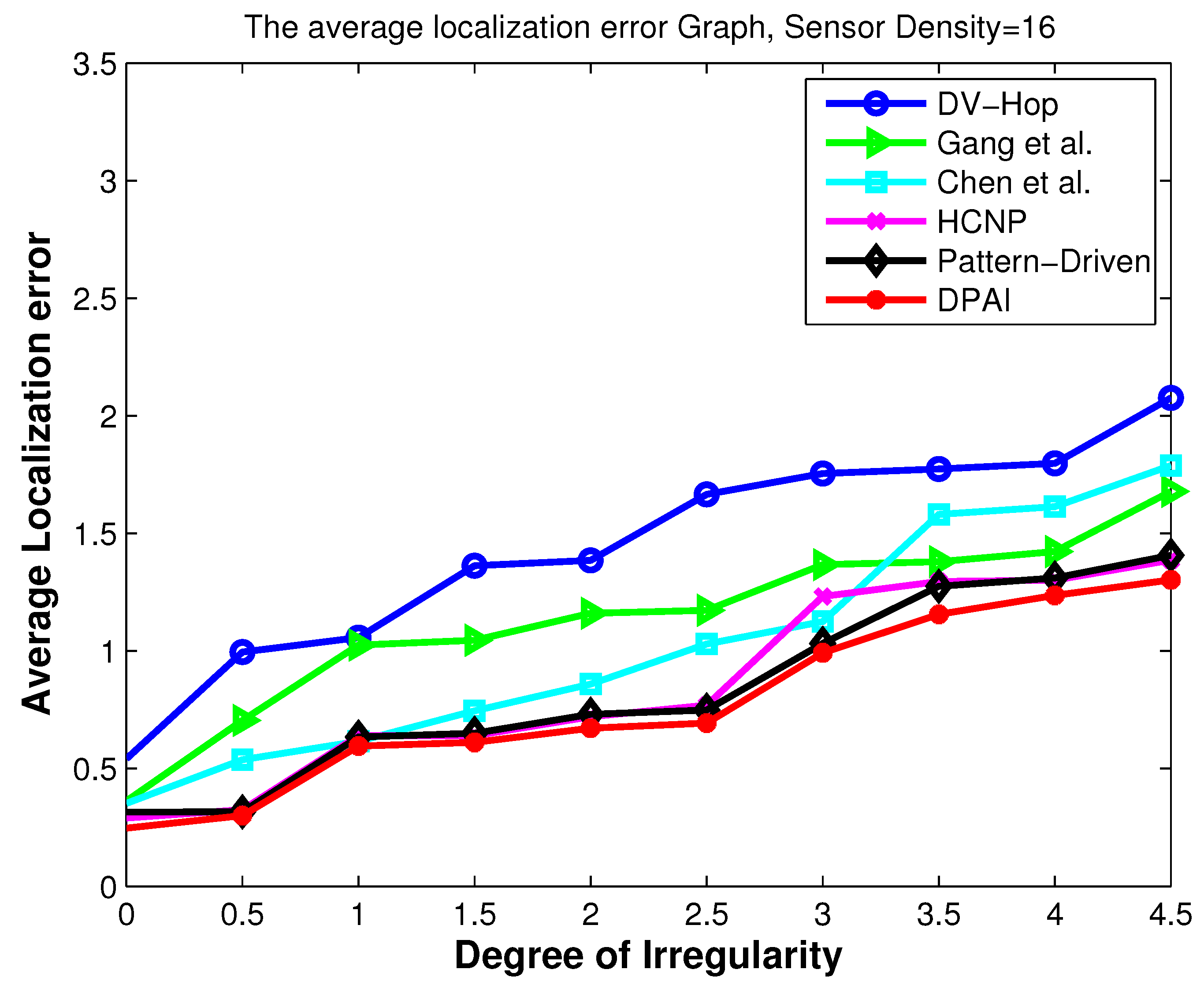
Figure 10.
Localization error vs. DOI.
Figure 10.
Localization error vs. DOI.
Figure 11.
Initial node deployment in isotropic network.
Figure 11.
Initial node deployment in isotropic network.
Figure 12.
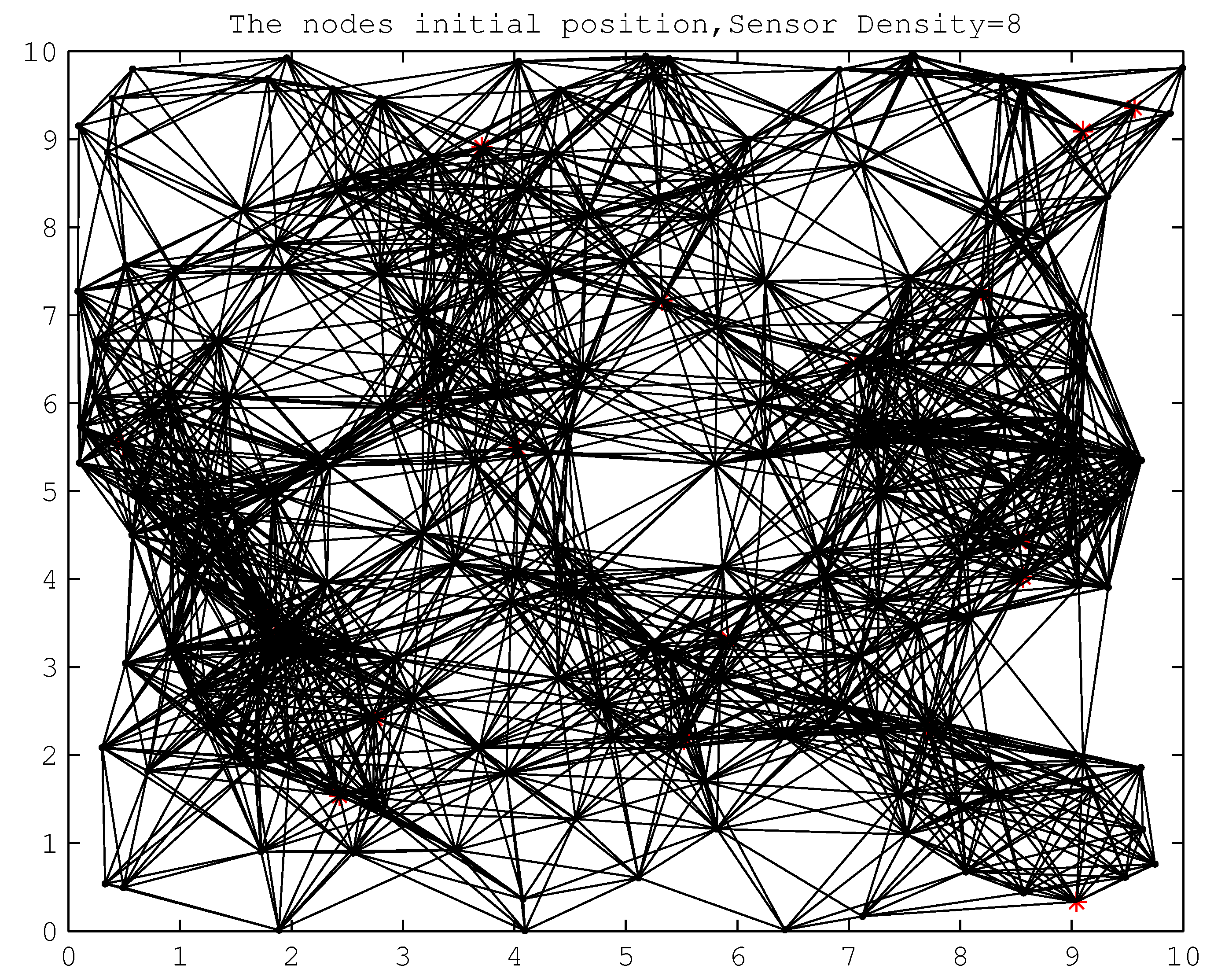
Initial node deployment in anisotropic O-shape network.
Figure 12.
Initial node deployment in anisotropic O-shape network.
Figure 13.
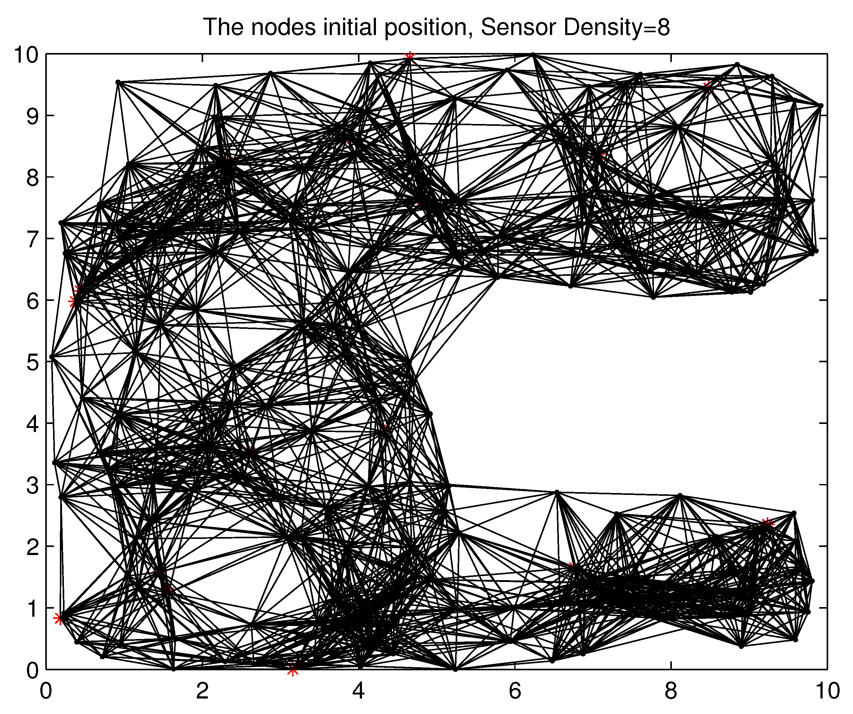
Initial node deployment in anisotropic C-shape network.
Figure 13.
Initial node deployment in anisotropic C-shape network.
Figure 14.
Irregular Radio Pattern when DOI=0.05.
Figure 14.
Irregular Radio Pattern when DOI=0.05.
Figure 15.
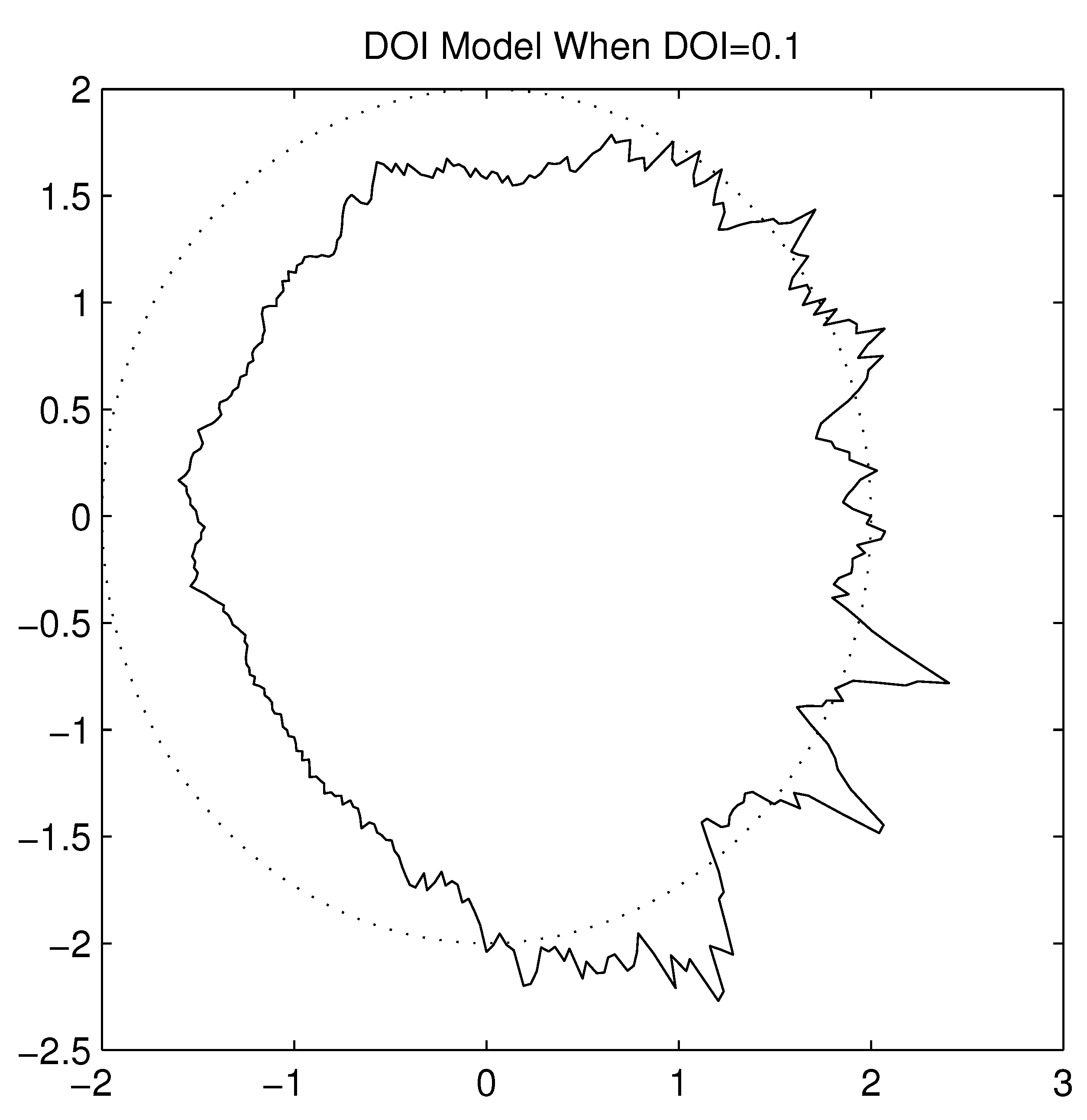
Irregular Radio Pattern when DOI=0.1.
Figure 15.
Irregular Radio Pattern when DOI=0.1.
5.1. Localization Error When Varying the Number of Anchors
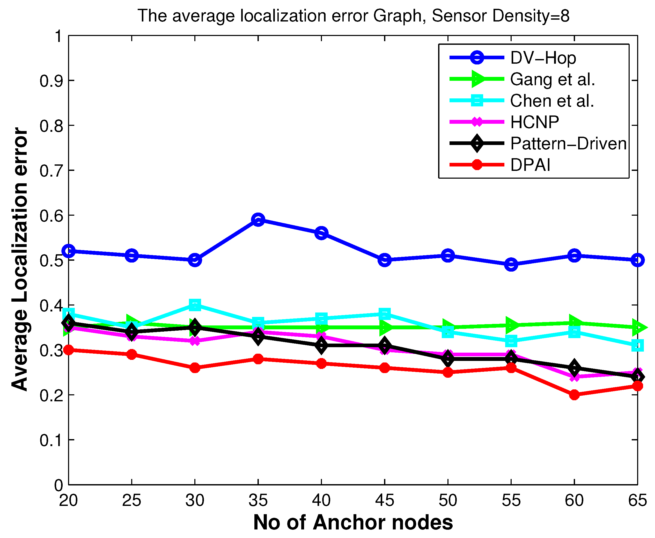
For the first experiment, we vary the number of anchors in sparse isotropic network (sensor density = 8) to study its impact on location accuracy.
Figure 4,
Figure 6 and
Figure 8 show that the localization accuracy of DPAI is better than others. For example, in
Figure 4 with 20 anchor nodes (which is 10% of total number of nodes), DPAI has an average localization error of about 0.3r, whereas in pattern-driven [
7] and HCNP [
11], the error is 0.37r and 0.36r respectively. We also observe that, as we increase the anchor numbers, the localization error of DPAI reduces from 0.3r to 0.21r. It can be seen from
Figure 6 and
Figure 8 that in anisotropic network, our proposed algorithm performs better than the pattern-driven algorithm and other algorithms. In fact, the performance of DV-Hop and other (except pattern-driven) algorithms in anisotropic network is random in nature and worst than in isotropic network. In O-shape and C-shape region, the transmission paths are more curved and the hop count based distance estimation from sensor nodes to anchor nodes is dramatically changed if the detoured transmission paths are treated in the same manner as in the isotropic network.
Our proposed algorithm outperforms others by using the angular value of the detoured transmission paths, i.e., the average hop distance among anchor nodes and the sensor nodes are adjusted according to the angle of the curved transmission paths. For the same sensor density, our scheme outperforms pattern-driven and other approaches even when the anchor to sensor ratio is as low as 10%, which signifies the cost effectiveness of our approach.
5.2. Localization Error When Varying the Sensor Density
Figure 5,
Figure 7 and
Figure 9 show the performance of our approach and other approaches when varying the sensor density. We vary the sensor density from 6 to 24. Effective localization remains a problem in sparse networks where the sensor density falls in the range of 6 to 15. Kleinrock and Silvester have proved in [
18] that 6 is the optimum sensor density to maintain the network connectivity. The localization problem in sparse networks deserves investigation, because lower sensor density implies lower deployment cost, smaller possibility of traffic jam, and radio interference.
It can be seen from
Figure 5,
Figure 7 and
Figure 9 that DPAI performs better than other schemes when the sensor density is 6, and as we increase the sensor density from 6 to 24, the localization error of DPAI as well as other approaches decreases. This is because, as the sensor density increases, the numbers of one hop neighbor nodes increases, so the per hop average distance calculation error decreases and the calculation error does not propagate to large number of hops. At a low sensor density such as 6 or 8, if the hop number is large, then there is a high possibility that the transmission path between two anchors is not straight but slightly curved in isotropic network. However, if the hop number is less (which occurs when the sensor density is high), then the path between two anchor nodes is almost straight and the average hop distance calculation becomes more accurate than before. By the value of the angle, we can determine whether the transmission path is straight or not and accordingly the average hop distance is calculated. In low sensor density isotropic network with no obstacle, some holes are created because of the low sensor density. In such situation, DPAI performs better because we calculated the average hop distance by utilizing the angle of the detour transmission path. In high density isotropic network, the localization error of DPAI approaches 0.22r (when the sensor density is 24) and in anisotropic network, the localization error is 0.25r for O-shape and 0.26r for C-shape respectively. For low density such as 8, the localization error of DPAI is near to 0.3r for isotropic network and below 0.35r for anisotropic network. According to [
2], this localization accuracy can satisfy the needs of many location dependent protocols and applications, such as geographical routing and tracking.
5.3. Localization Error When Varying the Degree of Irregularity (DOI)
Radio irregularity is a common and non-negligible phenomenon in wireless sensor networks [
19]. It results in irregularity in radio range and variations in packet loss in different directions, and is considered as an essential reason for asymmetric links as viewed by upper layers in the protocol stack. The parameter Degree Of Irregularity (DOI) is used to denote the irregularity of the radio pattern. It is defined as the maximum radio range variation per unit degree change in the direction of radio propagation. When the DOI is set to zero, there is no range variation, resulting in a perfectly circular radio model. To get a better idea of how this DOI parameter affects signal propagation characteristics,
Figure 14 and
Figure 15 show the radio patterns generated in simulation with DOI values set to 0.05 and 0.1 respectively. The DOI model is a good start to model signal irregularity. However, it does not model interference in real devices well. Since the DOI model is based on an absolute communication range, it assumes that within the inner range, the signal is very strong and can always be received correctly, while beyond the outer range there is no signal at all. This binary pattern is not true in reality.
To address the issue of radio irregularity in wireless sensor network, we utilized Radio Irregularity Model (RIM) [
19] in our simulation. This model bridges the discrepancy between spherical radio models used by simulators and the physical reality of radio signals and also verify the presence of radio irregularity using empirical data obtained from the MICA2 platform. RIM takes into account both the non-isotropic properties of the propagation media and the heterogeneous properties of devices.
In isotropic radio models, the received signal strength is usually represented with the following formula:
To reflect the two main properties of radio irregularity, namely non-isotropic and continuous variation, RIM adjusts the value of path loss models in (9) based on DOI values, resulting in the following formula:
Here
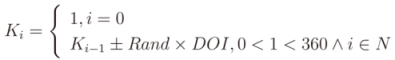
Ki is a coefficient to represent the difference in path loss in different directions. Specifically,
Ki is the
ith degree coefficient, which is calculated in the following way:
where ∥K0 −K359∥ ≤ DOI
It is possible to generate 360 Ki values for the 360 different directions, based on (12), by randomly fixing a direction as the starting direction represented by i =0. For the direction that does not have an integer value of angle from the start direction, the interpolation of the Ki value has been taken based on the values of the two adjacent directions that have integer angles from the starting direction.
where,
s= ⎣
i⎦ ∧
t = ⌈
i⌉
mod360 ∧ 0 <
i < 360 ∧
i ![Jsan 02 00025 i021]() N
N The variance of received signal strength in RIM in different directions fits the Weibull [
20] distribution. The Weibull distribution can be used to model natural phenomena such as variation of wind speed, scattering of radiation,
etc. The Rayleigh distribution, which is commonly used for modeling multi-path fading in wireless communication, is a special case of the Weibull distribution.
Due to the difference in hardware calibration and battery status, received signal strength can be different from two sending nodes of the same type. RIM introduces a second parameter named VSP (Variance of Sending Power), which is defined as the maximum percentage variance of the signal sending power among different devices, to account for such a difference. The new signal sending power is modeled by the following equation:
Thus with the two parameters, DOI and VSP, the RIM model can be formulated as follows:
With the help of the RIM model, we explore the impact of radio Irregularity of our proposed algorithm (DPAI).
In this experiment, we investigate the impact of irregular radio patterns on the precision of localization estimation. It is intuitive that irregular radio patterns can affect the network topologies resulting in irregular hop count distributions. We can see, in
Figure 10, how this inaccurate estimate directly contributes to localization error as the DOI increases. When DOI increases, it means the number of neighbors around a sensor node decreases, and as a result it is very likely that the shortest transmission path from one sensor node to another is more detoured than before. In that case our algorithm shows more robustness than other algorithms because of the angular value based average hop distance calculation. Our algorithm adapts to different detoured transmission path according to dynamic value of the angle and thus calculates the distance between an anchor node and a sensor node more accurately.
Figure 10 shows the localization error when varying DOI in isotropic network when the sensor density is 16. Obviously, in anisotropic network, which itself provides additional radio irregularity in the form of different obstacle shapes, more localization errors will be introduced as the DOI increases.

 , where dij is the straight line distance between the anchor node i and j, hj is the hop segment number between the anchor nodes i and j. Another algorithm in [10] calculates the error eij as
  , where
  is the estimated distance between anchor nodes i and j,
  is is the Euclidean distance between anchor i and j. The average hop distance is finally adjusted by
  where m is the closest anchor node to anchor node i and HopSizei is calculated as
  where (xi, yi) (xj, yj) are the coordinates of anchor node iand j and hij is the number of hops between anchor iand j. The Algorithms [9,10] made improvements on distance estimation and localization of the DV-Hop algorithm. There are still some disadvantages in the improved algorithms, such as no obvious improvement on localization accuracy, especially when the transmission route is not straight but detoured.
 where si is the ith sensor node. All sensor nodes are uniformly and independently deployed in a square area A = L× L. Such a random deployment results in a 2D Poisson distribution of sensors with sensor density
  . All sensors are assumed to be homogeneous and stationary and omnidirectional. Therefore the network can be seen as static or regarded as a snapshot of mobile ad hoc sensor networks. In order to simplify the discussion, we are not concerned with the issues of energy consumption and robustness of sensor nodes. We believe that these missing issues do not invalidate the correctness of the proposed method.


 and the real location (xi, yi) to the communication range of sensor nodes. In this paper, the average localization error is expressed relative to the radio range r. The average localization error △ of the sensor network, which is composed of |VS| sensor nodes, is expressed as follows:


 N
N