Extracting Main Center Pattern from Road Networks Using Density-Based Clustering with Fuzzy Neighborhood

Abstract

The spatial pattern is a kind of typical structural knowledge that reflects the distribution characteristics of object groups. As an important semantic pattern of road networks, the city center is significant to urban analysis, cartographic generalization and spatial data matching. Previous studies mainly focus on the topological centrality calculation of road network graphs, and pay less attention to the delineation of main centers. Therefore, this study proposes an automatic recognition method of main center pattern in road networks. We firstly extract the main clusters from road nodes by improving the Density-Based Spatial Clustering of Applications with Noise (DBSCAN) with fuzzy set theory. Moreover, the center area is generated with road meshes according to the area ratio with the covering discs of the main clusters. This proposed algorithm is applied to the road networks of a monocentric city and polycentric city respectively. The results show that our method is effective for identifying the main center pattern in the road networks. Furthermore, the contrast experiments demonstrate our method’s higher accuracy.

1. Introduction

The spatial pattern is a kind of typical structural knowledge, which reflects the inherent distribution characteristics and interrelations of geospatial entities. With structural knowledge, people can better understand and perceive the regional geographical environments [1,2,3,4]. The main purpose of spatial pattern recognition is to mine structural knowledge that conforms to human spatial cognition, which can effectively improve the availability of spatial data (i.e., data enrichment) [1,2,3]. Spatial pattern recognition has attracted more and more attention because of its important theoretical significance and application value in the fields of spatial data mining, spatial analysis and reasoning, cartographic generalization, and spatial data matching and updating [1,2,3,4,5,6].

According to the level of detail, the implicit spatial structural knowledge (i.e., spatial patterns) can be classified into three categories: local, medium and global [6,7]. Global knowledge is used to depict the overall characteristics of a region, which could help us to discern different geographic features easily. Usually, the urban road network is regarded as the skeleton of the city, which contains rich and multi-level spatial patterns [3,4,8]. Previous research on the spatial pattern recognition of road networks mainly focus on the grids [3,5,9,10], roundabouts [11,12,13], and strokes [3,14], seldom solve the problems of global and complex patterns such as global rings, global stars, city centers and urban built-up areas [3,15,16,17,18].

The city center is a typical element of the urban spatial structure [19], and the accurate boundary identification of the city center becomes vital in many applications. In the field of urban analysis, the city center functions as a nucleus of both economic and social activities within the city. Related studies have investigated topics such as retail development [20], employment [21], commercial districts [22,23,24] and social networks [25,26,27]. These studies can support policymakers to plan the city properly. In the domain of cartographic generalization, to preserve the spatial pattern of the map elements, the higher order graphical phenomenon (e.g., city center in this study) needs to be extracted beforehand [3]. For instance, the center pattern itself can be used to express the macroscopic city structures [17,24,28], and provide locating points to represent a city when the map scale decreases continuously. Besides, the center pattern is also the basis for the identification of other macroscopic distribution patterns, such as the global rings [15] and radial pattern [16].

As an exemplar of higher order semantics in road networks, the city center is vaguely defined. Most research focuses on the topological centrality of the network graph [29,30,31]. Jiang and Claramunt [32] abstracted the road networks into a dual graph and calculated the topological centrality based on graph theory to extract central vertex of a graph. However, Heinzle and Anders [3] believed that a polygon would be a better representation of the center in the detailed dataset and they extracted the center area using a two-step method. Firstly, the local centers were identified by clustering the centroids of the road blocks. Then, the combination of density and centrality of the clusters was used to filter potential center areas. This method is designed for the monocentric city, and it is difficult to apply in the cities with complex structures.

The expansion of a city causes changes in the urban structure. For example, there might be some sub-centers formed around the main center, or a new main center might be designed directly. The main centers are the most active areas and always described as the “heart of the city” [19]. Therefore, the number of main centers determines the global structure as monocentric or polycentric. Extracting main centers from the road networks is conducive to understanding the essential characteristic of a city and mainly helps to: (1) provide the basis for the complex pattern recognition (such as large rings); (2) find locating points for the graphic simplification; (3) support location query and navigation; (4) aid decision making in the structural and functional planning of a city.

We are focused on main center identification in this study. Referring to [3,17,28], there are always denser roads in a more active region, meaning that city centers are always located in the denser areas of the road networks. According to [17,24], the spatial distribution of road networks and road intersections is approximate, so the density of road networks can be measured by the road nodes, here including road intersections and ending points. Spatial clustering is effective in detecting the denser areas of the dataset [33] and researchers have adopted Density-Based Spatial Clustering of Applications with Noise (DBSCAN) in the vague region delineation [26,27,34]. In this study, the DBSCAN is improved with fuzzy neighborhood to identify main clusters (the densest and extensively connected clusters) from road nodes. Subsequently, the center areas are delineated based on the covering discs and road meshes.

Concerning the sections hereinafter, Section 2 gives an overview of related work. In Section 3, we describe the main center recognition algorithm based on an improved clustering method. Section 4 presents case studies of both a monocentric city and polycentric city. Finally, we conclude this paper and describe future work in Section 5.

2. Related Works

The recognition of city center areas is critical to urban structure and function analysis, and has drawn great attention from researchers. Studies such as those of Lynch [35] and Le et al. [36] argued that the range of the city center is fuzzy, and citizens could sense the city center. Furthermore, References [37,38] investigate the citizens’ perceptions and thus to derive the approximate range of the city center. The results show that these methods are available for cognitive region delineation, but it is difficult to verify the representativeness of the interviewees.

In contrast, extracting city centers from geographic data is more objective and practicable. Various models to delineate the city center have been developed using different data sources, mainly including the (1) index-based method, (2) density-based method, and (3) clustering-based method.

• The index-based method defines the city center by a simple or comprehensive indicator. For instance, Luscher and Weibel [39] extracted the city center from the topological datasets such as land cover and points of interest (POIs) with defined knowledge by participant experiments. Zhu and Sun [23] considered spatial proximity and attribute similarity in the delineation of city center from commercial land-use data. The index system is constructed according to the data source and the application, which always leads to different understandings of the “city center.”
• The density-based method mainly adopts a smooth density surface and the isolines to outline the center area. Hollenstein and Purves [25] explored the city cores through user-generated content and described the city cores using geo-referenced data with kernel density estimation (KDE). Yu et al. [22] provided a recognition method of a central business district (CBD) using the statistical aggregation of the socio-economic point data within network space. Yang et al. [24] proposed a commercial-intersection KDE, which combines road intersections with KDE to identify CBDs based on POIs. The density-based method is intuitive and the center areas are smooth, but it is difficult to determine the best bandwidth in the applications. Besides, there might be scattered areas due to the slightly higher density values than the threshold.
• The clustering-based method means that the data needs to be clustered first and then the boundary of the clusters is constructed using the convex hull, chi-shape, Delaunay triangle, Voronoi diagram, and so on. Yu et al. [40] analyzed the urban landscape pattern with an object-based method, in which urban objects were clustered by portioning Minimum Spanning Tree and then the clusters were delineated by the convex hull. Sun et al. [27] sought to combine the DBSCAN algorithm and Voronoi diagram to identify multiple city centers and delineate their precise boundaries from location-based social network data. Hu et al. [26] defined urban areas of interest (AOI) as the areas within a city that attract the attention of people, and a combination of DBSCAN and chi-shape was employed to identify AOI from the geo-tagged data. Gao et al. [34] used the same method to define the core regions and concluded that data-synthesis-driven approach has a clear advantage that it can be repeated for a wide field at flexible spatial scales.

Comparatively, the clustering-based method is concise and not restricted by research units, so it is commonly used in the vague region extraction. Among the existing spatial clustering algorithms [33], DBSCAN has received much attention due to its high computational efficiency in large databases, ability in discovering clusters with arbitrary shape, and no requirements of a pre-set number of clusters [33,41]. Therefore, the “DBSCAN+outline” method is more common in the third category of the city center identification methods [26,27,34]. However, further research demonstrates that DBSCAN will result in scattered and fragmented hot spot patterns, which are unfavorable to main center extraction. Therefore, in this study, we attempt to improve the DBSCAN method with fuzzy set theory and extract the main centers from the road networks.

3. Methods

The overview of the proposed main center pattern recognition approach is described in Figure 1, including two steps. The first step is introduced in Section 3.1, mainly to discover the main clusters in the road nodes by the density-based clustering with fuzzy neighborhood (DBCFN). We first give the fundamental concepts and the clustering principle of DBCFN, and then explain how to set the parameters. The second step is to establish the cluster boundaries (see Section 3.2), including the cover discs construction of the main clusters and boundary generation based on the road meshes.

3.1. Main Clusters Extraction

In DBSCAN, clusters are discovered based on the difference in distribution density. Figure 2 depicts the principle and analysis of the DBSCAN. With two global parameters, epsilon (Eps) and minimum points (MinPts), the points are divided into three categories: core, non-core and noise [41], as shown in Figure 2a. When determining whether a point belongs to a cluster, the DBSCAN uses a binary membership. Thus, all points contribute equally to the density calculation for a core point, regardless of the distance. As shown in Figure 2b, the core point p₁ is in a denser region than p₂, but DBSCAN considers the density values of the two cores the same. The inaccurate estimation of density is unfavorable to extracting the core clusters. Additionally, the DBSCAN algorithm also overlooks the fact that an object may belong to multiple clusters with various membership degrees, and consequently, small clusters (where the number of neighboring points in a cluster is smaller than MinPts) are produced. As shown in Figure 2c, when MinPts = 5, if q is classified to the left cluster already, then the right cluster with p₂ as the core only has four neighboring points, which indicates a small cluster. The small clusters would lead to a fragmented pattern.

For the main center pattern, we need to extract the densest clusters with more neighbouring points (i.e., main clusters). Moreover, the number of main clusters should be determined by the number of main centers in a city. Therefore, we will improve the DBSCAN from two aspects: firstly, the fuzzy membership is used to replace the binary membership, and then the clustering strategy is modified by considering the sharing points and cluster number.

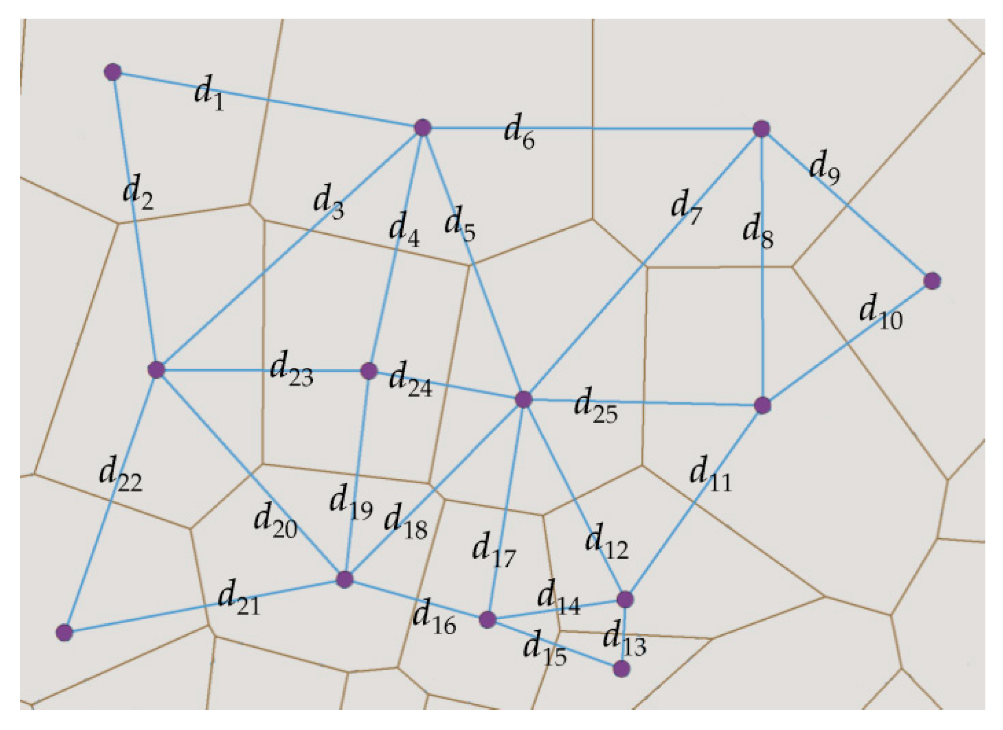
3.1.1. Basic Concepts of the DBCFN

Fuzzy set theory has been applied to addressing various problems on geospatial information where the results of a binary approach are undesirable [42,43]. According to fuzzy set theory, an object can have varying grades of membership in multiple sets [44]. This is similar to spatial clustering in which a point can belong to multiple clusters with different degrees of membership. The membership function assigns membership to candidate points with the values in [0,1]. Among the two common membership functions (i.e., linear type and exponential type), the exponential one can measure the aggregation features of points better [45]. Therefore, the DBCFN is developed based on the exponential membership function, and the concepts are as follows:

Definition 1.

Fuzzy membership degree. The membership degree refers to the degree that q belongs to p. In DBSCAN, the membership degree, noted as M_c(p,q), can be formally represented by

$$M_c\left(p,q\right)=\{\begin{array}{c}1,\hspace{1em}\hspace{1em}\hspace{1em}\hspace{1em}\hspace{1em}d\left(p,q\right)<Eps\\ 0,\hspace{1em}\hspace{1em}\hspace{1em}\hspace{1em}\hspace{1em}\hspace{1em}\hspace{1em}\hspace{1em}\mathrm{otherwise}\end{array},$$

(1)

where d(p,q) is the Euclidean distance between p and q. In fuzzy set theory, the fuzzy membership degree M_f is defined as

$$M_f\left(p,q\right)=\exp \left[-{\left(\frac{d\left(p,q\right)}{Eps}\right)}^2\right].$$

(2)

The value of M_f falls in the interval of (0, 1]. Equation (2) shows that the longer the distance, the smaller the M_f. This characteristic is consistent with the First Law of Geography, which contributes to cluster identification.

Figure 3 depicts two types of membership. In Figure 3a, two points with different distances (but less than Eps) from p have the same membership degree, and contribute to the density of p equally. However, as shown in Figure 3b, the improved fuzzy membership decreases continuously as the distance increases, so that the two points with different distances contribute differently to the density of p.

Definition 2.

Fuzzy set cardinality: the sum of the fuzzy membership degrees of all the points {q₁, q₂,…, q_t} within the Eps neighborhood of p, i.e.,

$$C_f\left(p\right)={{\displaystyle \sum }}_{i=1}^t{M}_f\left(p,q_i\right),$$

(3)

where C_f (p) characterizes the density of the area where p is located, and the higher the C_f (p), the denser the area is surrounding p.

Definition 3.

Fuzzy core point. The point p is referred to as a fuzzy core point if C_f (p) > ε₁. ε₁ is the threshold for deciding whether a point is a fuzzy core point. In DBSCAN, the critical condition for point p to be a fuzzy core point is that MinPts points that are located at a distance of Eps from p exist. Thus, C_f (p) is equal to MinPts/e according to Equation (3), where e is the base of the natural logarithm (as shown in the following expression). Here, ε₁ is defined as

$${\epsilon }_1=\mathsf{\lambda }\times \frac{MinPts}{\mathrm{e}},$$

(4)

where λ is an adjustment factor (λ = [1, 2, 3…]). The larger λ is, the higher the density around the core point, and the higher the probability for the cluster to become the main center.

Definition 4.

Directly density-reachable. If point p is a core and point q satisfies the condition of M_f (p,q) > ε₂, then point q is directly density-reachable from point p. In DBSCAN, the critical condition of being directly density-reachable is that the distance between p and q is Eps. Therefore, M_f (p,q) = 1/e according to Equation (2). Thus, parameter ε₂ is set to 1/e.

In addition, the definitions of density-reachable and density-connected are the same as the definitions that apply to the DBSCAN algorithm.

3.1.2. Principle of the DBCFN

The DBCFN is designed to extract the densest and largest set of density-connected points. In this algorithm, two visited flag arrays, namely an outer-array and an inner-array are defined to avoid small clusters. The outer-layer array records whether the core point has been visited, while the inner-layer array records whether the non-core point has been visited. The inner-array will reset each time the cluster is completed. The purpose of separately recording a visited flag is to ensure that all non-core points will be visited during each clustering process. In some situations, a point may belong to several clusters. We argue that these clusters should be merged because the shared points show spatial relations among these clusters. By this way, we can derive the largest connected area, which contributes to identification of the main clusters.

Let M be the number of main centers and m be the number of clusters. The clustering process is described as follows:

• Input the parameter MinPts and Eps, and calculate M_f and C_f of the points;
• Calculate parameter ε₁ with a certain λ, and search for the core points;
• Search for the largest set of density-connected points with parameter ε₂ from a core point;
• Repeat Step 3 until all core points have been visited, and allocate the points that have not been classified into any cluster as noise;
• Merge the clusters that share common points and record m; and
• If m is greater than M, then turn to Step 2 with the parameter λ + 1; else, break.

The main clusters are determined by the clustering results in which m is closest to M during the above procedure.

3.1.3. Parameters Setting

In DBCFN, the parameters of MinPts and Eps, the same as in DBSCAN, need to be set in advance. For the points without any special geographical sense, researchers always choose the k-dist method to set these two parameters [33,41]. Specifically, MinPts is set by the formula of MinPts = k ≈ ln(N), where N is the number of road nodes; then, the distance from each other point is calculated, and the k-nearest distances of all points are chosen to be plotted at equal intervals ascending in order; the distance value at the sharp change in slope is Eps. This method supports a heuristic way to set these two parameters. However, Eps by this method is an approximate value, and the sharp change point is hard to determine when the slope changes all the way smoothly.

Essentially, the clusters are the areas that are denser than the mean level of the dataset. To set the Eps automatically and objectively, we propose an average method of proximity distances. In computational geometry, the Voronoi diagram is used to divide a plane according to the nearest neighbor principle. Additionally, the other way around, we can determine the proximity of two points by their Voronoi neighbor [46]. In the Voronoi diagram, if the Voronoi areas of two nodes are disjoint, the adjacent coefficient is 0; otherwise the adjacent coefficient is 1. Then the Eps is defined as

$$Eps=\frac{1}{n}\times {\displaystyle \sum }_{i=1}^N{\displaystyle \sum }_{j=1}^N{d}_{ij}\times v{n}_{ij},$$

(5)

where d_ij and vn_ij are the distance and adjacent coefficient between p_i and p_j respectively; n is the number of the adjacent coefficient that is equal to 1. Considering the points in Figure 4 as an example, Eps = (d₁+d₂+…+d₂₅)/25.

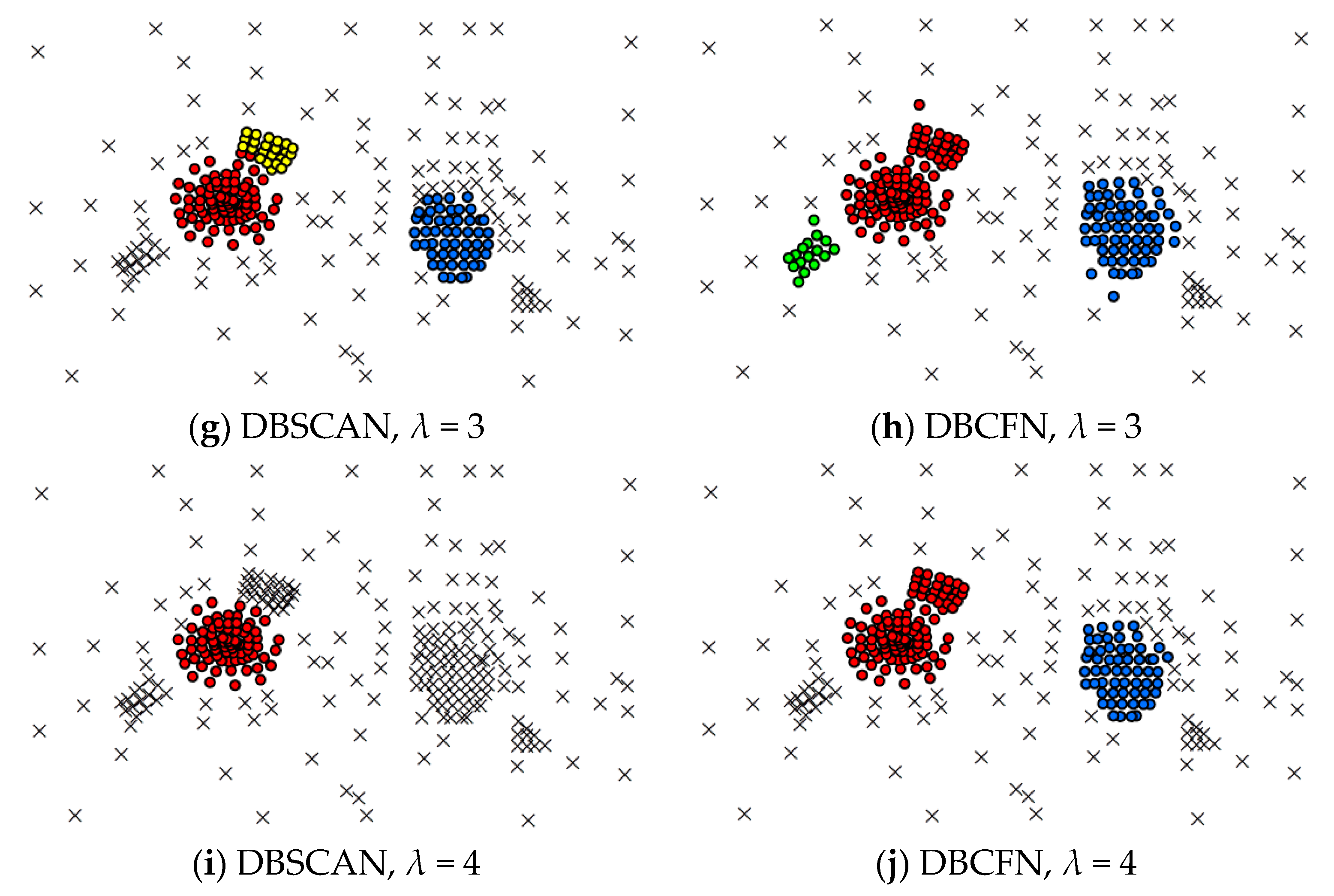
3.1.4. Comparison Analysis

In order to illustrate the advantages of DBCFN in detecting the main clusters, we took the simulated roads as an example to conduct a comparison experiment. The DBSCAN method was performed using the strategy in Section 3.1.2, and the condition for core points is that there are at least λ × MinPts points in its Eps neighborhood. By this way, we can compare these two methods more sufficiently. Figure 5 shows the dataset and clustering results. In human perception, there are two main centers, A and B, as shown in Figure 5a.

From Figure 5c–j, we can see that the numbers of clusters by these two methods present a decreasing trend with the increase of λ. In DBSCAN, the numbers of clusters are 4, 3, 3, and 1; in Figure 5g, the red cluster breaks into two clusters; Figure 5i shows that the yellow cluster and blue clusters disappeared at the same time, which does not agree with the expected results. In DBCFN, the numbers of clusters are 4, 4, 3, and 2; when λ = 4, two main clusters are obtained as shown in Figure 5j, which conform to human perception. Compared with DBSCAN, our method performs better in the main center identification.

3.2. Main Center Area Delineation

As the main clusters have been identified from the road nodes, one more step is necessary to delineate the areas (polygons) based on those clusters. This process is also called the crisp boundary formation, which makes sense for many applications such as cartographic visualization, query processing, and urban planning [39]. Among the standard algorithms of boundary construction, the convex hull [40], chi-shape [26] and Delaunay Triangulation [23] are the typical boundaries that are formed by the points in the original dataset, without considering the influence range of the outer points of the cluster. However, the region generated by covering discs (CD) [47], Voronoi diagram [27], and region growing algorithm [39] contains the influence area of the outer points and Galton called it extended footprints [47].

In this study, we chose the CD method to construct the boundary of the clusters, because the covering discs not only contain all the points with an equal influence radius, but also reflect the cluster shape smoothly. The boundary of the cluster is constructed by the following two steps: (1) create buffers for the points except for the noise with a radius of Eps; and (2) merge the buffers of the points that belong to one cluster. According to the principle of DBCFN, the maximum distance from the core points to the outer points is Eps. Thus, there will be no holes within the cluster boundary by this method. Figure 6 shows an example of the main center delineation.

From Figure 6a, we can see that the shape of CD is similar to the outline of the clusters. However, in the spatial pattern recognition of the road networks, the buffer area has no explicit administrative meaning. Besides, if the clusters are near the district border, the buffer area might extend beyond the study area. Thus, we use the road mesh (minimum polygons enclosed by road lines) to represent the center area. For a certain CD zone, the mesh can be divided into two categories, including central mesh and outer mesh. A mesh’s type is determined by the indicator of area ratio (AR), which is defined as

$$A{R}_{ij}=\frac{S{O}_{ij}}{S{M}_i},$$

(6)

where SO_ij is the overlapped area of the i-th mesh and j-th cluster buffer; SM_i is the area of the i-th road mesh. The range of AR is [0,1]. The higher AR means that it is more likely for a mesh to become a part of the center. In this study, if a mesh has an AR larger than 0.5, it would be defined as the central mesh for the j-th cluster. All the central meshes that belong to the j-th cluster are merged into one polygon.

The main center areas are represented by the red polygons in Figure 6b. They are composed of the actual blocks that have explicit geographical significance, which is especially important in the spatial query and cartographic representation.

The key technologies in the proposed main center recognition method contain Voronoi graph construction, DBCFN and CD generation. Therefore, the time complexity of this method is determined by these three aspects. The computation required to construct the Voronoi graph is O(N^2), where N is the number of road nodes. The DBCFN method has an approximate time complexity of O(N^2). Generating the CD can be accomplished in time complexity of O(NlogN). Therefore, the complexity of the proposed method is O(N^2). The time complexity analysis of this method points out that the main clusters extraction contributes greatly to the computational cost.

4. Experiments and Analysis

The proposed methods were applied to delineate the main city centers based on the road networks of Xi’an and Shenzhen. These two cities are located in northwest and southeast respectively in China. Among them, Xi’an is studied as the case of the monocentric city (single-center city), and Shenzhen is researched as the case of the polycentric city (multi-center city). Since the algorithm steps are the same, the experiment of the monocentric city will be presented as the main example.

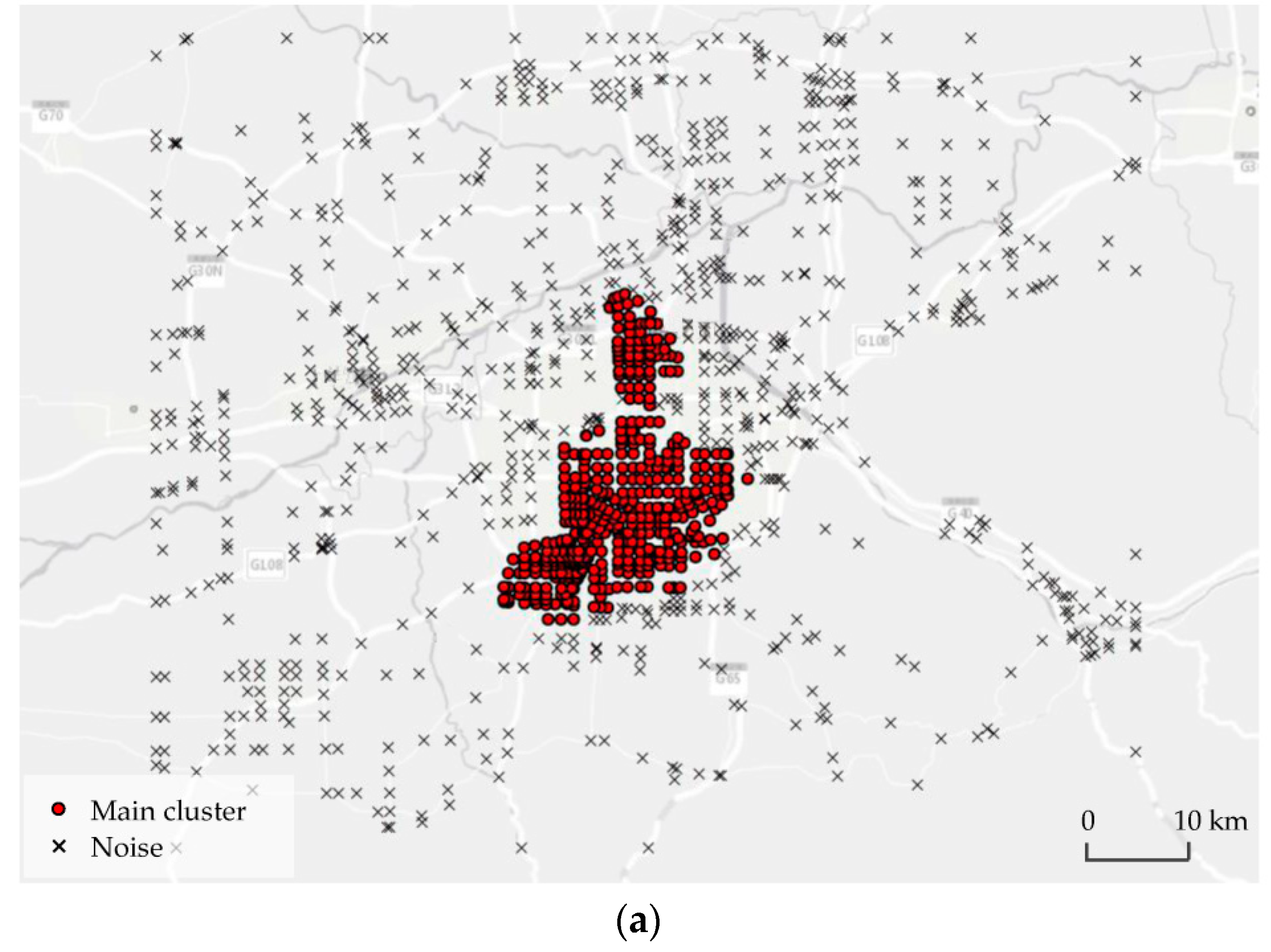
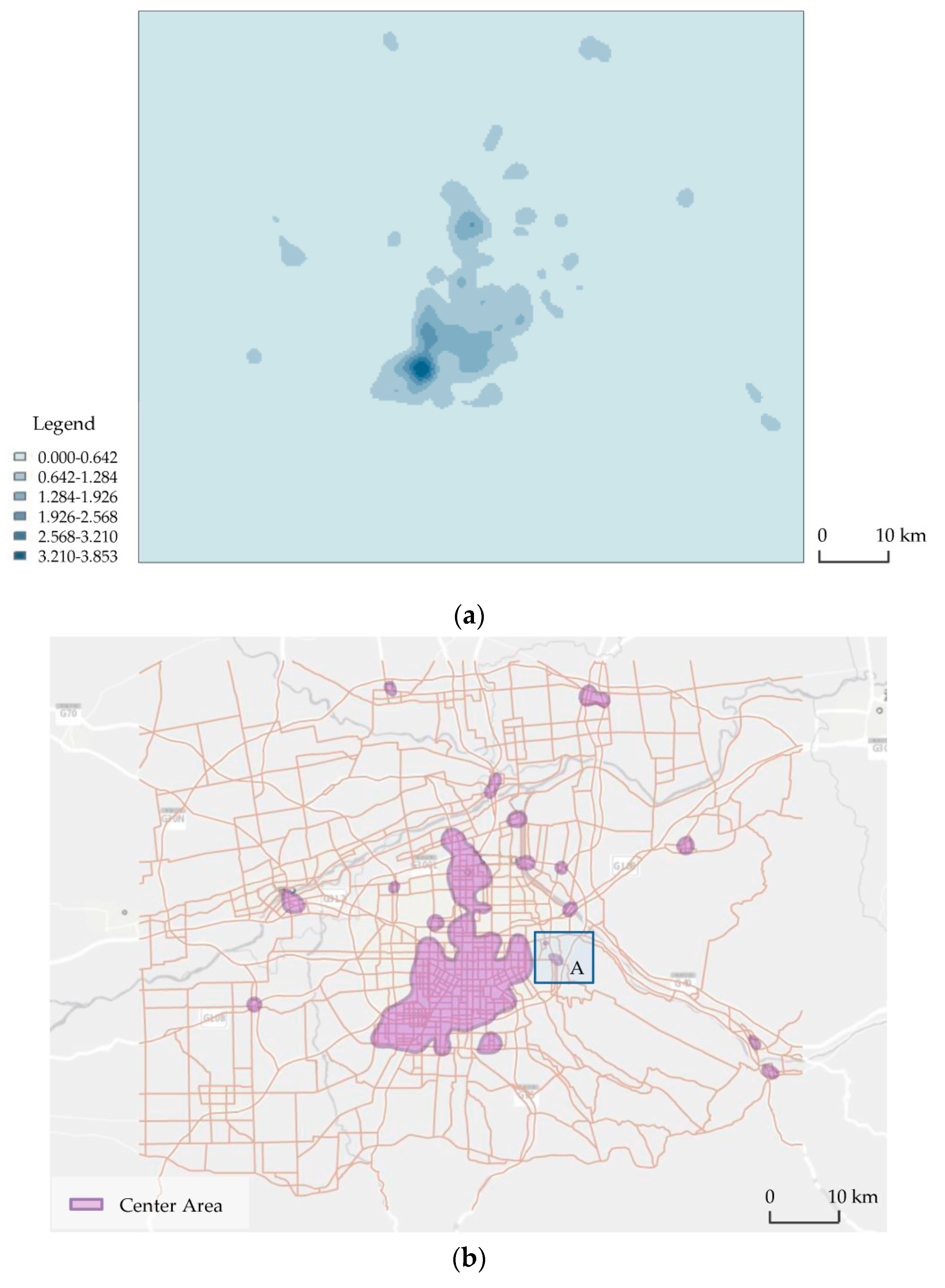
4.1. Case of the Monocentric City

Xi’an is a traditional city with a long history, functioned as the capital of Shanxi Province. It is a typical single-center city with visible grids in the center area. Figure 7 shows the study area and road networks in Xi’an. There are 2053 road segments and 1245 road nodes, so the MinPts is equal to ln(1245) ≈ 7. Then, the Voronoi diagram was constructed to derive the adjacency list of the nodes. Next, the Eps was calculated according to the Equation (5), and the result is 2459.6 m.

Figure 8 depicts the recognized results of Xi’an. In a case of monocentric city, the parameter M (number of main centers) is set to one. Thus, the main clusters were identified by DBCFN, represented by red points in Figure 8a. The number of the clusters is exactly equal to 1 when λ = 4. Based on the results of the main clusters, the covering discs were created with Eps, as the blue area shown in Figure 8b. Moreover, we used the overlay analysis to calculate the spatial relationship between the road mesh and the covering discs. Finally, we obtained the main center areas comprised of the merged road meshes, as shown in Figure 8b.

The recognized center is a contiguous area with the road segments as the boundary, which is explicable in geographical context. Figure 9 shows a detailed analysis of the recognized center. We can see that, the recognized center is located in several joint districts, mainly including Weiyang District, Lianhu District, Beilin District and Yanta District. There are many important facilities in this recognized area, such as the municipal government, railway stations (Xi’an, Xi’anbei, and Xi’anxi), universities (Xidian, Northwest, and Xi’an Jiao Tong) and historical sites (Xi’an Circumvallation, and Great Wild Goose Pagoda). It can be concluded that the recognized main center takes on the role of the political, economic, traffic, and cultural center of Xi’an.

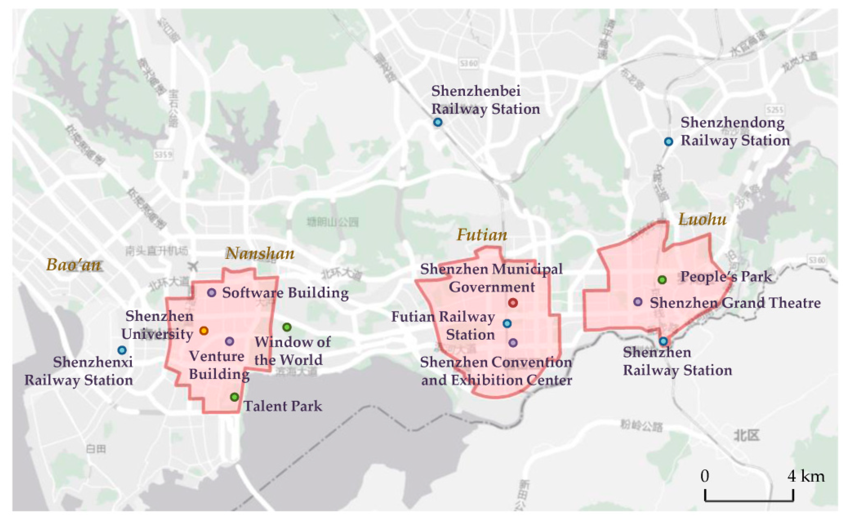
4.2. Case of the Polycentric City

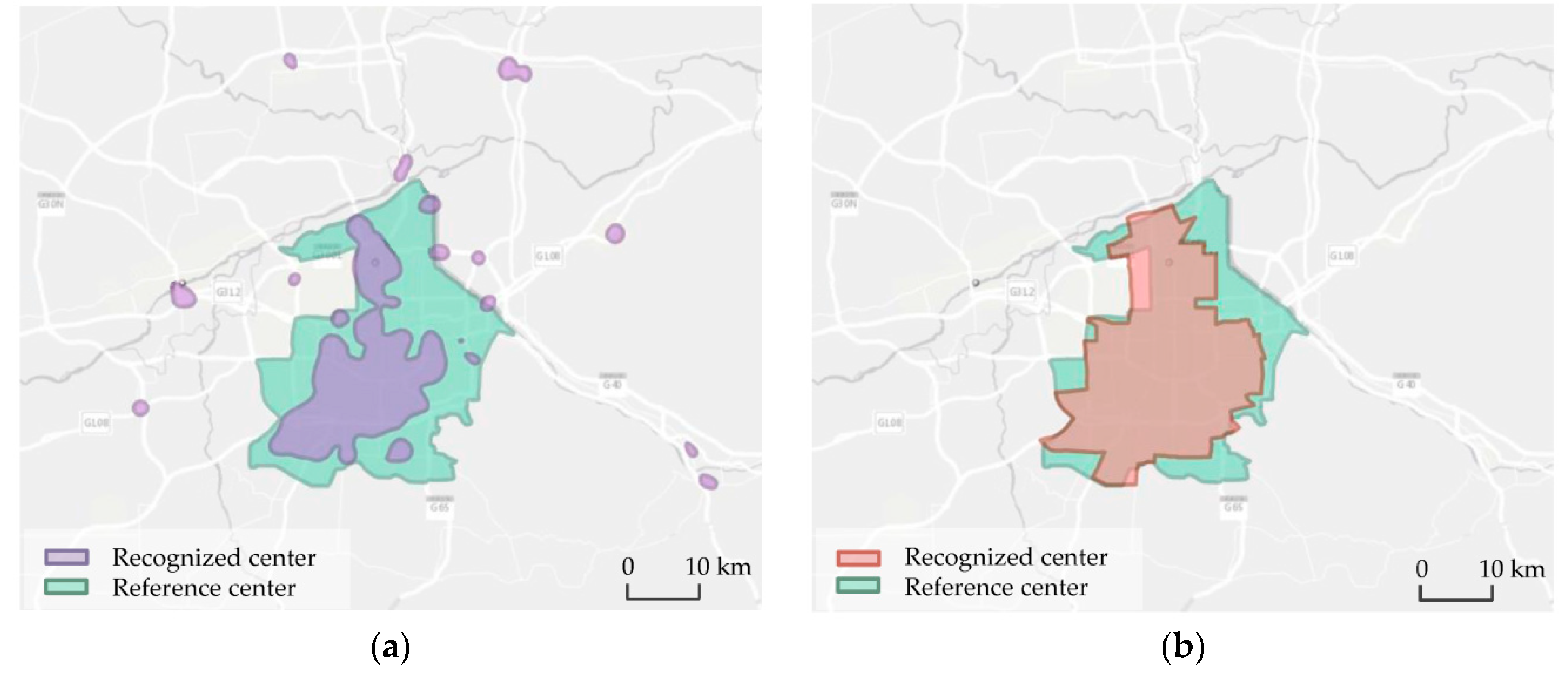
Shenzhen is a new immigrant city that has been developed in recent years due to the government’s supportive policies. There are 10 districts in Shenzhen, and three of them are functioned as the centers of the city, namely Futian, Luohu, and Nanshan. Therefore, the number of the main centers is set to three. Figure 10 shows the study area and road networks in Shenzhen, which exhibits a free distribution pattern with sub-grids.

There are 2607 road segments and 1566 road nodes in Shenzhen’s test data. The calculated values of MinPts and Eps are 7 and 1286.8 m, respectively. By using the proposed method, we extract three main clusters when λ = 6. Moreover, three polygons are delineated as main centers. Figure 11 shows the recognized results. From Figure 11b, we can see that a small part of the left covering discs is beyond the land area, and the right covering discs is across two cities (Shenzhen and Hong Kong). These phenomena are unreasonable in the geographical cognition of the city center. However, by using the road meshes, these deficiencies are remedied and we obtain a more explicit center area.

Figure 12 shows the analysis of the recognized center areas in Shenzhen. In the left center, there are the Shenzhen University, Venture building and Software building, suggesting that this area focuses on science and technology. The middle center mainly undertakes the political and economic function according to the facilities such as municipal government and the convention and exhibition center. As for the right area, it is a trade center and cultural entertainment center because of the commercial malls, parks and recreational facilities. The recognized results are corresponding to the Nanshan District, Futian District, and Luohu District from west to east, respectively. Besides, the right center has been extended west into Futian District, demonstrating the achievements of constructing the united center of “Futian-Luohu.”

4.3. Comparison

Montello et al. (2014) and Gao et al. (2017) hold the view that the boundaries of the cognitive regions (such as city centers, city settlement areas or other regions of interest) are typically substantially vague [34,48]. Consequently, there are spatial uncertainties in the city center extracted from the spatial data. To further illustrate the advantages of the proposed algorithm for main center pattern, contrast experiments of the “Kernel density + Contour” method [22] were performed with the experimental data. The key to the application of this method lies in the setting of the bandwidth h which is mainly dependent on the aggregation degree of the spatial distribution. According to Section 3.1.3, the bandwidth can be set to Eps, the same as in DBCFN.

In Xi’an, a continuous kernel density surface was calculated with h = 2459.6 m. The mean and standard deviation were calculated as 0.158 and 0.288 respectively. Thus, the contours were generated with the threshold 0.734. Figure 13 shows the results of KDE and center areas in Xi’an.

In Shenzhen, a continuous kernel density surface was calculated with h = 1286.8 m. Then, the contours were generated with the threshold 2.038 (mean 0.402 and standard deviation 0.818). Figure 14 shows the results of KDE and center areas in Shenzhen.

Some characteristics of the identified results by contrast method and our method are summarized in

Table 1. Characteristics of the recognized results by two methods in two cities.

City	Method	Number of Polygons	Number of Holes	Boundary Extent
Xi’an	Contrast method	18	0	Within the city
	Proposed method	1	0	Within the city
Shenzhen	Contrast method	45	2	Beyond the city
	Proposed method	3	0	Within the city

. For the main center identification, the contrast method has a poor performance: (1) there are so many trivial areas (as shown in box A in Figure 13b and Figure 14b) caused by the local high density, actually there are no centers. This deficiency is especially obvious in Shenzhen because so many “0” pixels outside of the study area are counted for the average of the kernel density, as shown in Figure 14a. Therefore, the computed mean and standard deviation is much lower than that of the real study area, leading to more polygons delineated as the center areas. (2) There would be holes in the center area, as shown in box B in Figure 14b. This is due to the locally lower values of the kernel density estimation. The holes in a center polygon not only go against human cognitive habits for fuzzy areas, but also increase the difficulty of the spatial computation and analysis. (3) The center area by the contrast method might be beyond the administrative boundary city (as shown in box C in Figure 14b), which is hard to explain in some applications. Comparatively, the proposed method can delineate the center areas that conform to the city structure.

In order to compare these methods objectively, a quantitative evaluation was performed based on the dataset of Xi’an. According to [39,49], we adopted the planning center area, which is defined by the Overall Urban Planning for Xi’an (2008–2020), as a reference. Figure 15 shows the overlay analysis between the recognized centers and reference center. Three evaluation indicators were employed in this study: the recall (R, the ratio of the area of overlapped center to the area of the reference center), precision (P, the ratio of the area of overlapped center to the area of recognized center) and F₁-score (harmonic mean of R and P).

The evaluation results of these two methods are presented in

Table 2. Comparison of the indices of the center recognition results.

Algorithm	R	P	F1-score
Contrast method	0.399	0.885	0.550
Proposed method	0.698	0.947	0.804

. Previous research shows that the computed F₁-score is in the range of 0.45~0.86 when taking the planning center as a reference [39]. Therefore, the recognized results by two methods are both effective. Further comparisons demonstrate that contrast method has the lower R (0.399) and lower P (0.885), and so the F₁-score is also lower (0.619). As for the proposed method, the R and P reach 0.698 and 0.947 respectively, so the F₁-score is high (0.804).

In general, the F₁-score of this method is 46.2% higher than that of the contrast method. Therefore, the center area recognized by the proposed method is significantly better than that by the contrast method. Fundamentally, this is because fuzzy membership can better represent the density characteristics of spatial points and is more applicable to the extraction of main center patterns.

Above analysis shows that the center patterns can be extracted efficiently with the premise that city center always locates on the denser areas of road networks. This is because the road networks, as one of the most important elements in urban space, can embody the essential structure of the city: the more active the region, the greater the road density and the more likely it is to become the center [3,17,28]. That is to say, the center pattern of the road networks are always closely related to the center patterns of the city. From this aspect, as long as there is a center pattern (monocentric or polycentric) in the study area, it can be recognized by our method. However, the differences between the recognized center and the planning/investigated center are inevitable due to the uncertainties in human cognition.

5. Conclusions

The city center is a typical semantic pattern of road networks, which plays a vital role in the city structure. To extract the main center patterns from road networks, we developed a two-step method. This method has several advantages in that: (1) fuzzy set theory is used to improve the DBSCAN, thus to distinguish the main clusters from the minor clusters with the increasing demand for a core point. (2) The “area of influence” is considered for all the points of the main cluster by using the CD method, and then the center area is refined based on the road mesh that has clear geographical sense. (3) The parameters can be determined by the dataset automatically, which can reduce uncertainties of the vague region delineation.

We apply this algorithm to road data of single-center pattern (Xi’an road networks) and multi-center pattern (Shenzhen road networks) to test its performance. The experimental results reveal that the proposed algorithm is capable of extracting main center areas that conform to spatial cognition: (1) the recognized centers reflect prominent aggregation pattern of the dataset; (2) the recognized centers are continuous areas without any holes; and (3) the overlapped degree with the planning center is much higher than that of the contrast method.

Further research will focus on three aspects. (1) Identify complex patterns such as large rings (i.e., global ring pattern in the road networks). According to the literature [3], the large rings always surround the city center. Therefore, the next step is extracting the circular roads, and then filtering the rings based on the spatial relationship with the main centers. (2) Extend the proposed method to the spatial pattern recognition of building groups. Urban buildings are primary spaces for people’s activities, and the spatial distribution of the urban buildings thus reflects the city structure [7]. The proposed method can be improved to delineate the geometrical centers from building groups. (3) Explore the relevance of cognition for spatial patterns. The recognized results can be further verified by investigating people’s perception of city centers. Additionally, this can be performed by the specific “drawing task” [48] or eye movement experiments [50].

References

1. Mackaness, W.; Edwords, G. The Importance of Modeling Pattern and Structure in Automated Map Generalization. In Proceedings of the Joint ISPRS/ICA Workshop on Multi-Scale Representations of Spatial Data, Ottawa, ON, Canada, 7–8 July 2002. [Google Scholar]
2. Steiniger, S. Enabling Pattern Aware Automated Map Generalization. Ph.D. Thesis, University of Zurich, Zurich, Switzerland, 2007. [Google Scholar]
3. Heinzle, F.; Anders, K.H. Characterizing Space via Pattern Recognition Techniques: Identifying Patterns in Road Networks. In Generalization of Geographic Information: Cartographic Modeling and Applications; Elsevier Ltd.: Amsterdam, The Netherlands, 2007; pp. 233–253. [Google Scholar]
4. Zhang, Q. Modeling Structure and Patterns in Road Network Generalization. In Proceedings of the ICA Workshop on Generalization and Multiple Representation, Leicester, UK, 20–21 August 2004. [Google Scholar]
5. Yang, B.; Luan, X.; Li, Q. An Adaptive Method for Identifying the Spatial Patterns in Road Networks. Comput. Environ. Urban Syst. 2010, 34, 40–48. [Google Scholar] [CrossRef]
6. Gong, X.; Wu, F. A Typification Method for Linear Pattern in Urban Building Generalization. Geocarto Int. 2016, 33, 189–207. [Google Scholar] [CrossRef]
7. Chaudhry, O.; Mackaness, W.A. Automatic identification of urban settlement boundaries for multiple representation databases. Comput. Environ. Urban Syst. 2008, 32, 95–109. [Google Scholar] [CrossRef]
8. Marshall, S. Streets & Patterns; Spon Press: London, UK, 2005. [Google Scholar]
9. Tian, J.; Song, Z.; Gao, F.; Zhao, F. Grid Pattern Recognition in Road Networks Using the C4.5 Algorithm. Cartogr. Geogr. Inf. Sci. 2016, 43, 266–282. [Google Scholar] [CrossRef]
10. He, Y.; Ai, T.; Yu, W.; Zhang, X. A Linear Tessellation Model to Identify Spatial Pattern in Urban Street Networks. Int. J. Geogr. Inf. Sci. 2017, 31, 1541–1561. [Google Scholar] [CrossRef]
11. Touya, G. A Road Network Selection Process Based on Data Enrichment and Structure Detection. Trans. GIS 2010, 14, 595–614. [Google Scholar] [Green Version]
12. Savino, S.; Rumor, M.; Zanon, M.; Lissandron, L. Data Enrichment for Road Generalization through Analysis of Morphology in the Cargen Project. In Proceedings of the 13th ICA Workshop on Generalization and Multiple Representation, Zurich, Switzerland, 12–13 September 2010. [Google Scholar]
13. Cui, X.; Wang, J.; Gong, X.; Wu, F. Roundabout Recognition Method Based on Improved Hough Transform in Road Networks. Acta Geod. Cartogr. Sin. 2018, 47, 1670–1679. [Google Scholar]
14. Yang, B.; Luan, X.; Li, Q. Generating Hierarchical Strokes from Urban Street Networks Based on Spatial Pattern Recognition. Int. J. Geogr. Inf. Sci. 2011, 25, 2025–2050. [Google Scholar] [CrossRef]
15. Heinzle, F.; Anders, K.H.; Sester, M. Pattern Recognition in Road Networks on the Example of Circular Road Detection. In Proceedings of the 4th Geographic Information Science, Münster, Germany, 20–13 September 2006; pp. 153–167. [Google Scholar]
16. Tian, J.; Zhang, B.; Wu, D. A New Method for Identifying Radial Pattern in Vector Road Networks. Geomat. Inf. Sci. Wuhan Univ. 2013, 38, 1234–1238. [Google Scholar]
17. Borruso, G. Network Density and the Delimitation of Urban Areas. Trans. GIS 2003, 7, 177–191. [Google Scholar] [CrossRef]
18. Zhou, Q. Comparative Study of Approaches to Delineating Built-Up Areas Using Road Network Data. Trans. GIS 2016, 19, 848–876. [Google Scholar] [CrossRef]
19. Murphy, R.E.; Vance, J.E. Delimiting the CBD. Econ. Geol. 1954, 30, 189–222. [Google Scholar] [CrossRef]
20. Lowe, M. The Regional Shopping Centre in the Inner City: A Study of Retail-led Urban Regeneration. Urban Stud. 2005, 42, 449–470. [Google Scholar] [CrossRef]
21. Redfearn, C. The Topography of Metropolitan Employment: Identifying Centres of Employment in a Polycentric Urban Area. J. Urban Econ. 2007, 61, 519–541. [Google Scholar] [CrossRef]
22. Yu, W.; Ai, T.; Shao, S. The Analysis and Delimitation of Central Business District Using Network Kernel Density Estimation. J. Transp. Geogr. 2015, 45, 32–47. [Google Scholar] [CrossRef]
23. Zhu, J.; Sun, Y. Building an Urban Spatial Structure from Urban Land Use Data: An Example Using Automated Recognition of the City Centre. ISPRS Int. J. Geo-Inf. 2017, 6, 122. [Google Scholar] [CrossRef]
24. Yang, J.; Zhu, J.; Sun, Y.; Zhao, J. Delimitating Urban Commercial Central Districts by Combining Kernel Density Estimation and Road Intersections: A Case Study in Nanjing City, China. ISPRS Int. J. Geo-Inf. 2019, 8, 93. [Google Scholar] [CrossRef]
25. Hollenstein, L.; Purves, R. Exploring Place through User-Generated Content: Using Flickr to Describe City Cores. J. Spat. Inf. Sci. 2010, 1, 21–48. [Google Scholar]
26. Hu, Y.; Gao, S.; Janowicz, K.; Yu, B.; Li, W.; Prasad, S. Extracting and Understanding Urban Areas of Interest Using Geotagged Photos. Comput. Environ. Urban Syst. 2015, 54, 240–254. [Google Scholar] [CrossRef]
27. Sun, Y.; Fan, H.; Li, M.; Zipf, A. Identifying the City Centre Using Human Travel Flows Generated From Location-Based Social Networking Data. Environ. Plann. B Plann. Des. 2016, 43, 480–498. [Google Scholar] [CrossRef]
28. Jiang, B.; Liu, X. Scaling of Geographic Space from the Perspective of City and Field Blocks and Using Volunteered Geographic Information. Int. J. Geogr. Inf. Sci. 2012, 26, 215–229. [Google Scholar] [CrossRef]
29. Porta, S.; Crucitti, P.; Latora, V. The Network Analysis of Urban Streets: A Primal Approach. Environ. Plan. B Plan. Des. 2006, 33, 705–725. [Google Scholar] [Green Version]
30. Crucitti, P.; Latora, V.; Porta, S. Centrality measures in spatial networks of urban streets. Phys. Rev. E 2006, 73, 036125. [Google Scholar] [CrossRef] [PubMed] [Green Version]
31. Jiang, B. A topological pattern of urban street networks: Universality and Peculiarity. Phys. A Stat. Mech. Its Appl. 2007, 384, 647–655. [Google Scholar] [CrossRef]
32. Jiang, B.; Claramunt, C. A Structural Approach to the Model Generalization of an Urban Street Network. Geoinformatica 2004, 8, 157–171. [Google Scholar] [CrossRef]
33. Liu, Q.; Deng, M.; Shi, Y.; Wang, J. A Density-Based Spatial Clustering Algorithm Considering both Spatial Proximity and Attribute Similarity. Comput. Geosci. 2012, 46, 296–309. [Google Scholar] [CrossRef]
34. Gao, S.; Janowicz, K.; Montello, D.R.; Hu, Y.; Yang, J.; Mckenzie, G.; Ju, Y.; Gong, L.; Adams, B.; Yan, B. A Data-Synthesis-Driven Method for Detecting and Extracting Vague Cognitive Regions. Int. J. Geogr. Inf. Syst. 2017, 31, 1245–1271. [Google Scholar] [CrossRef]
35. Lynch, K. The Image of the City; MIT Press: Cambridge, MA, USA, 1960. [Google Scholar]
36. Le, T.; Abrahart, R.; Aplin, R.; Priestnall, G. Town Centre Modelling Based on Public Participation. In Proceedings of the CUPUM 05, Computers in Urban Planning and Urban Management—9th International Conference, London, UK, 29 June–1 July 2005. [Google Scholar]
37. Montello, D.R.; Goodchild, M.F.; Gottsegen, J.; Fohl, P. Where‘s Downtown: Behavioral Methods for Determining Referents of Vague Spatial Queries. Spat. Cognit. Comput. 2003, 3, 185–204. [Google Scholar]
38. Borruso, G.; Porceddu, A. A Tale of Two Cities: Density Analysis of CBD on Two Midsize Urban Areas in Northeastern Italy. In Geocomputation and Urban Planning; Springer: Berlin/Heidelberg, Germany, 2009; pp. 37–56. [Google Scholar]
39. Lüscher, P.; Weibel, R. Exploiting Empirical Knowledge for Automatic Delineation of City Centres from Large-Scale Topographic Databases. Comput. Environ. Urban Syst. 2013, 37, 18–34. [Google Scholar] [CrossRef]
40. Yu, B.; Shu, S.; Liu, H.; Song, W.; Wu, J.; Wang, L.; Chen, Z. Object-based Spatial Cluster Analysis of Urban Landscape Pattern Using Nighttime Light Satellite Images: A Case Study of China. Int. J. Geogr. Inf. Sci. 2014, 28, 2328–2355. [Google Scholar] [CrossRef]
41. Ester, M.; Kriegel, H.-P.; Sander, J.; Xu, X. A Density-based Algorithm for Discovering Clusters in Large Spatial Databases with Noise. In Proceedings of the KDD 1996, Portland, OR, USA, 2–4 August 1996; pp. 226–231. [Google Scholar]
42. Roberts, A. Integrating High Resolution Remote Sensing, GIS and Fuzzy Set Theory for Identifying Susceptibility Areas of Forest Insect Infestations. Int. J. Remote Sens. 2005, 26, 4809–4828. [Google Scholar]
43. Cui, X.; Wang, J.; Gong, X.; Zhao, Y. Hotspot Area Recognition by Using Fuzzy Density Clustering and Bidirectional Buffer. Geomat. Inf. Sci. Wuhan Univ. 2019, 44, 84–91. [Google Scholar]
44. Zadeh, L. Fuzzy Sets as a Basis for a Theory of Possibility. Fuzzy Sets Syst. 1978, 1, 3–28. [Google Scholar] [CrossRef]
45. Nasibov, E.N.; Ulutagay, G. Robustness of Density-Based Clustering Methods with Various Neighborhood Relations. Fuzzy Sets Syst. 2009, 160, 3601–3615. [Google Scholar] [CrossRef]
46. Chen, J.; Yan, C.; Zhao, R.; Zhao, X. Voronoi Neighbor-based Self- adaptive Clipping Model for Mobile Maps. Acta Geod. Cartogr. Sin. 2009, 38, 152–155. [Google Scholar]
47. Galton, A.; Duckham, M. What Is the Region Occupied by a Set of Points? Lect. Notes Comput. Sci. 2006, 4197, 81–98. [Google Scholar]
48. Montello, D.R.; Friedman, A.; Phillips, D.W. Vague Cognitive Regions in Geography and Geographic Information Science. Int. J. Geogr. Inf. Sci. 2014, 28, 1802–1820. [Google Scholar] [CrossRef]
49. Heikinheimo, V.; Minin, E.D.; Tenkanen, H.; Hausmann, A.; Erkkonen, J.; Toivonen, T. User-generated geographic information for visitor monitoring in a national park: A comparison of social media data and visitor survey. ISPRS Int. J. Geo-Inf. 2017, 6, 85. [Google Scholar] [CrossRef]
50. Keil, J.; Mocnik, F.-B.; Edler, D.; Dickmann, F.; Kuchinke, L. Reduction of map information regulates visual attention without affecting route recognition performance. ISPRS Int. J. Geo-Inf. 2018, 7, 469. [Google Scholar] [CrossRef]
Figure 1. Schematic diagram of the main center pattern recognition.
Ijgi 08 00238 g001
Figure 2. (a) Principle of the Density-Based Spatial Clustering of Applications with Noise (DBSCAN); (b) density calculation for the core points; (c) two clusters share a common point.
Ijgi 08 00238 g002
Figure 3. Membership functions: (a) binary type; (b) exponential type.
Ijgi 08 00238 g003
Figure 4. The calculation example of Eps.
Ijgi 08 00238 g004
Figure 5. Simulated data and contrast results.
Ijgi 08 00238 g005aIjgi 08 00238 g005b
Figure 6. (a) Covering discs (CD) boundaries of the clusters; (b) main center areas.
Ijgi 08 00238 g006
Figure 7. The study area and road networks in Xi’an.
Ijgi 08 00238 g007
Figure 8. (a) Main cluster of the road nodes in Xi’an; (b) main center pattern in Xi’an.
Ijgi 08 00238 g008aIjgi 08 00238 g008b
Figure 9. Analysis of the recognized center pattern in Xi’an.
Ijgi 08 00238 g009
Figure 10. The study area and road networks in Shenzhen.
Ijgi 08 00238 g010
Figure 11. (a) Main clusters of the road nodes in Shenzhen; (b) main center patterns in Shenzhen.
Ijgi 08 00238 g011aIjgi 08 00238 g011b
Figure 12. Analysis of the recognized center patterns in Shenzhen.
Ijgi 08 00238 g012
Figure 13. (a) Results of kernel density estimation of road nodes in Xi’an; (b) center areas by the contrast method in Xi’an.
Ijgi 08 00238 g013
Figure 14. (a) Results of kernel density estimation of road nodes in Shenzhen; (b) center areas by the contrast method in Shenzhen.
Ijgi 08 00238 g014
Figure 15. (a) The overlay diagram of the recognized center by contrast method and the reference center; (b) the overlay diagram of the recognized center by proposed method and the reference center.
Ijgi 08 00238 g015