A Hybrid of Differential Evolution and Genetic Algorithm for the Multiple Geographical Feature Label Placement Problem

Abstract

Label placement is a difficult problem in automated map production. Many methods have been proposed to automatically place labels for various types of maps. While the methods are designed to automatically and effectively generate labels for the point, line and area features, less attention has been paid to the problem of jointly labeling all the different types of geographical features. In this paper, we refer to the labeling of all the graphic features as the multiple geographical feature label placement (MGFLP) problem. In the MGFLP problem, the overlapping and occlusion among labels and corresponding features produces poorly arranged labels, and results in a low-quality map. To solve the problem, a hybrid algorithm combining discrete differential evolution and the genetic algorithm (DDEGA) is proposed to search for an optimized placement that resolves the MGFLP problem. The quality of the proposed solution was evaluated using a weighted metric regarding a number of cartographical rules. Experiments were carried out to validate the performance of the proposed method in a set of cartographic tasks. The resulting label placement demonstrates the feasibility and the effectiveness of our method.

1. Introduction

The cartographic label placement problem is a classical issue of map production, and is also a combinatorial optimization problem [1]. As an important factor in cartography, labels in a map convey discrete spatial and non-spatial information. The readability and usability of a map are directly related to the quality of its annotation.

Given that the label placement is a fundamental problem in map production and graphical information systems, the cartographic community has tried to propose cartographical rules to guide the process of label placement, which aim to generate high-quality results and productions especially for automatic cartography maps. Some of this work was started by Yoeli [2], who proposed a set of principles for high-quality labeling, including the relationships that a particular feature and label should be aesthetic, label and feature visibility, and label-feature association. Imhof [3] presented three general principles that should be followed. They are that labels should be legible, the map conveys information clearly, and maintains an aesthetic balance. Most literature considered in this paper follows the principles proposed by Imhof for a proper design.

While the cartographical rules proposed might enable a well-established label placement to visually deliver the spatial information, algorithms for automatic adjustment and combination of the labels ensuring aesthetical and readability of the maps are non-trivial. Most attention [4,5] has been given to the point-features cartographic label placement (PFCLP) problem, which has been proved to be a non-deterministic polynomial-time hard (NP-Hard) problem. Different algorithms such as simulated annealing algorithm [6], zero-one integer linear programming [7,8], and greedy algorithm [9,10] are used to solve the objective function of the PFCLP problem. Verner et al. [11] used genetic algorithm to obtain good results for some instances. Azamathulla et al. [12] developed and compared two models based on the genetic algorithm and linear programming applied to real-time reservoir operation. From their results, they found the genetic algorithm to be superior to linear programming. Li et al. [13] proposed a label model based on the region of movability, which defines a complete conflict-free search space for label placement. Yamamoto and Lorena [14] presented a constructive genetic algorithm to obtain good results for cases up to 1000 points. The results were further improved by Gomes and Lorena [15] by using the constructive genetic algorithm that utilizes the notion of masking to preserve optimal subsequences in chromosomes. Their computational results validate the algorithm when applied to instances up to 5046 points.

While the above methods achieve promising results for the label placement problem, less attention has been given to line and area features. Cartographic label placement for line features involves point positioning mode [16] and line mode. The key for line mode is how to define the locating line of the line feature. In the work by Wolff et al. [17], the curvature of the lines along which the labels are placed is bounded from above by the curvature of a circle with radius r. Their algorithm has been proved by an experiment showing that it runs in sub-quadratic time and generally yields good results in practice. Sun et al. [18] presented a method that firstly produces a candidate curve along the line feature by a vector-oriented algorithm and then computes all of the candidate locations. Other research includes the efforts by Wu et al. [19] who proposed a new grid algorithm in contrast to traditional vector-based methods. Given the line features, the cells passed by a line are computed, and cells parallel to them are selected as the lower boundary of the text.

For area labeling, the placement algorithms also include point mode and skeleton line mode according to the particular shape and area of the features [20]. The original attempt with the area mode is to place the labels inside a constrained area so that they intersect the center of gravity of the area without coming too close to the border lines [2]. Most of the recent literature [21] has adopted the so-called skeleton method in which the labels should be placed on skeleton curves of the areas. Rylov and Reimer [22] introduced a novel and efficient algorithm for labeling area features externally, i.e., outside the polygonal boundary, and claimed to achieve efficient label placement that is close to the quality of manually produced cartographic products.

The development of simultaneous label placement of all types of cartographic features (e.g., point, line and area features) has emerged in recent years. Edmondson et al. [23] developed scoring rules for point, line and area candidate positions, and presented an algorithm by combining simple cartographic heuristics with effective stochastic optimization techniques. While the label placement method attempts to achieve a practical efficiency, the neglect of the relationship between the labels and the features might lead to ambiguity. Kakoulis et al. [24] presented a fast and simple technique based on a general framework for assigning labels to the edges of graph drawings. However, in their implementation, line features are limited to straight lines. Zhang and Harrie [25] presented a method that combines text and icon label placement in a real-time manner, which is achieved by labeling point and line features, and attached an icon to each of the area features randomly.

Most of the studies cited above focus on label placement for a single type of feature. However, this ideal setting is not satisfied in actual cartographical and map browsing scenarios, where a variety of cartographic features exist ranging from point, to line and to area features. On the other hand, while some methods do exist for joint label placement for point, line and area features, a major concern is the limitation of their algorithms in searching for the global optimum to fit the cartographical rules. In this paper, we present an approach to the problem of multiple geographical feature label placement (MGFLP) within a unified framework. To achieve high quality label placement, the genetic algorithm is leveraged to solve the global minimum of the objective function defined for MGFLP. Most importantly, for improving the efficiency of the genetic algorithm (GA), the GA is hybridized with discrete differential evolution (DDE). The differential evolution is a global search algorithm based on the population of a set of possible solutions (“chromosomes”). It has the ability to learn from individual populations and is adaptive in the searching direction [26]. By controlling the search direction of the differential mutation, the DE algorithm can yield better results [27]. This hybridization combines the strengths of both GA and DDE, which enables an effective and efficient solution of the MGFLP problem as demonstrated in the results of our experiments.

2. Candidate-Position Generation and Quality Evaluation Model

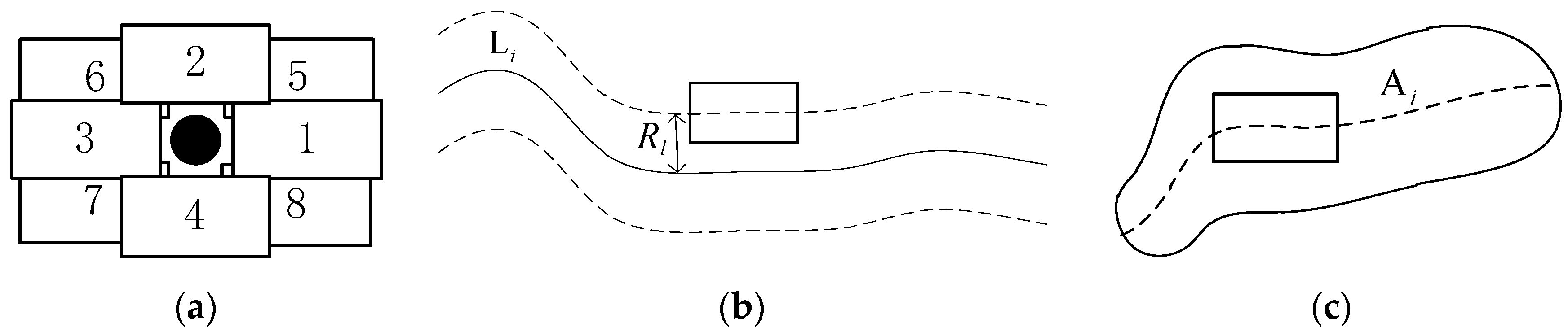
2.1. Candidate-Position Generation

Given a spatial dataset of point, line and area features, we first identify a set of candidate locations for their labels. Although ideally the number of candidate positions of each feature approximates infinity, the labeling principles should be considered when candidate positions are generated, so the set of candidate positions is limited. The labeling models are developed for each type of feature based on cartographic design principles and are described below.

The candidate positions of point features are discretely distributed around the point symbol. The candidate positions for point labels include four, five, eight and more positions. To ensure the effectiveness and the efficiency of labeling, eight candidate positions are chosen as shown in Figure 1a.

The labeling model of line features adopts the vector of parallel lines as the locating line. The center point of the candidate label rectangle slides along the specific parallel line, and the letters of the label are inscribed such that they are aligned consistently with the trend of the lines. Here, the parallel lines are classified into two types, depending on the angle $\beta$ between direction of the line feature and the horizontal direction. Consider $\beta \in \left[45°,135°\right]$, as the angle of a left–right parallel line, otherwise it defines a top–bottom parallel line. For the top–bottom parallel lines, the sequence of letters is aligned from left to right, whereas, for the left–right ones, the sequence is from top to bottom. To select candidate positions, the direction of the parallel lines is first considered in which the top and right parallel lines have higher priority, and the distance between the center of the label rectangle and the midpoint of the line feature is calculated. A smaller distance corresponds to a higher priority for the candidate rectangle.

A candidate-position model of line features is given in Figure 1b. For a given line feature $L_i$, a buffer distance is defined as $R_l$. For calculating the first candidate position, we generate the lines parallel to the feature, and then select an endpoint of the top buffer line or the right buffer line, which are only considered here as the center of the initial candidate rectangle. According to the curvature and the coordinates of the point, the label rectangle is displaced to be parallel to the line feature. The remaining candidate positions are generated by moving the initial position left and right to the top buffer line and up or down to the right buffer line with the offset distance defined as $s=l/\left(k-1\right)$, where $l$ is the length of line feature and $k$ is the number of candidate positions.

The labeling model for area features is divided into point mode and line mode. For the point mode, the area features are abstracted as points and labeled according to the method of point features. For the line mode, as shown in Figure 1c, the label is placed on the reference line inside the polygon. Here, the reference line represents the tendency of the area feature. The remaining problem is the extraction of the reference lines inside the polygon, which is the major concern of the area label placement problem. In practice, we use the common horizontal cutting midpoint method [28] to extract the skeleton of the polygon as the reference line.

2.2. Quality Metric

The essence of the labeling quality metric is a quantitative expression of the cartographic label placement, which is taken as the guidance of the labeling and directly affects the results. The metric refers to analyzing various aspects that affect the quality the labeling, and quantifies that effect of these aspects on the labeling quality as a function. Through the quality metric, the score of the labeling quality can be obtained, and the quality of the labeling can be quantitatively determined. The score determines the choice of the label position, which is also the premise of the optimization of the labeling algorithm. Therefore, the rationality of the quality evaluation function determines the final quality of the labeling.

An effective and rationalized metric for solutions of the MGFLP problem should take full account of the relationship among point, line, and area features. Based on the placement principles, four factors were chosen in our metric. The notations and definitions of the factors and the metric are listed in

Table 1. Notations and definitions.

Notation	Description
$N$	Total number of labels of the map
$S_{i1}$	Score of label conflict factor for the ith label, $i\in \left[1,N\right]$
$S_1$	Score of label conflict factor of the map
$C_{i1}$	Number of overlaps between the $i$th label and the other labels
$S_{i2}$	Score of label-feature conflict factor for the $i$th label
$S_2$	Score of label-feature conflict factor of the map
$C_{i2}$	Number of overlaps between the $i$th label and other features
$C$	Number of the label rectangles on the map
$S_{i3}$	Score of label non-ambiguity factor for the $i$th label
$S_3$	Score of label non-ambiguity factor of the map
$D_i$	Minimum Euclidean distance between the $i$th label rectangle and the center of the line feature or the center of the skeleton line of the area feature
$D_{max}$	The maximum Euclidean distance between the label and the center of the line feature or the center of the skeleton line of the area feature
$S_{i4}$	Score of label priority factor for the $i$th label
$S_4$	Score of label priority factor on the map
$\alpha$	The angle between the line of the center of label rectangle and point feature with the horizontal line
$S_i$	Score of quality evaluation for the $i$th label
$S_j$	Score of the $j$th factor, $j\in \left[1,2,3,4\right]$
$W_j$	Weight of each impact factor
$S$	Score of quality evaluation for the cartographic label placement

.

• Label conflict

Label conflict in the MGFLP problem refers to the overlap between any labels in the map. Label conflict is an important factor affecting the quality of the map. The number of overlapping labels is the criterion to evaluate the quality of placement. Overlapping labels may be accepted or not. When overlaps are not accepted, the maximum scale factor for the label size is found such that labels are generated without conflict [29]. Minimizing the number of conflicts [30] and maximizing the number of conflict-free labels [31] are two approaches to solve the problem when overlaps are allowed. Here, the chosen objective was to minimize the number of overlapping labels when overlaps are accepted. The core formula of the label conflict factor is:

$$S_{i1}=\{\begin{array}{c}0, C_{i1}=0\\ 1, C_{i1}\ne 0\end{array}$$

(1)

$$S_1={{\displaystyle \sum }}_{i=1}^N{S}_{i1}$$

(2)

• Label-feature conflict

Label-feature conflict is the overlap between labels and features. Label-feature conflict is often inevitable, however, it is also allowable. Accordingly, the solution of the label placement problem is formulated to reduce the label-feature conflict. Point features have a high priority for reduction of the label-feature conflict; that is, to avoid missing map information, labels cannot overlap point features. To decrease the overlap of labels with line and area features, the label-feature conflict functions can be written as:

$$S_{i2}=\{\begin{array}{c}0, C_{i2}=0\\ \frac{C_{i2}}{C},C_{i2}\ne 0\end{array}$$

(3)

$$S_2={{\displaystyle \sum }}_{i=2}^N{S}_{i2}$$

(4)

• Label non-ambiguity

Label non-ambiguity refers to the degree that the map user is certain of the association between a label and the corresponding feature. The label should clearly indicate the feature to be labeled without confusion with other features. This evaluation factor relates to the positions of labels for line and area features. The distance between the label and the feature is the only indicator of the factor. A smaller distance indicates a lower ambiguity and greater degree of association between label and feature. For line features, the distance is defined using the minimum Euclidean distance between the center of the label and the line feature, and, for area features, the distance is defined using the minimum Euclidean distance between the center of the label and the skeleton line. The factor is calculated from:

$$S_{i3}=\{\begin{array}{l}1, D_i=D_{max}\\ \frac{D_i}{D_{max}}, 0<D_i<D_{max}\\ 0,D_i=0\end{array}$$

(5)

$$S_3={{\displaystyle \sum }}_{i=1}^N{S}_{i3}$$

(6)

• Label priority

Label priority refers to the orientation between the label and the corresponding feature. Each feature has an ideal label position according to the reading habits of the user. The label priority has a greater impact for point features, where only the factor of the point-feature label needs to be evaluated. For point features, the label position with highest priority should be selected if it is marked separately. If considering the other rules in the whole map, the position with highest priority also should be selected. The evaluation criteria are scored according to the eight candidate positions of point features, $P_d\left(d=1,2,\dots ,8\right)$, corresponding to the candidate label positions in Figure 1a. The factor can be expressed as:

$$S_{i4}=\{\begin{array}{c}0.25,d\in (1,5)\\ 0.5,d\in (2,6)\\ 0.75,d\in (3,7)\\ 1,d\in (4,8)\end{array}$$

(7)

$$S_4={{\displaystyle \sum }}_{i=1}^N{S}_{i4}$$

(8)

Given the four factors described above, the final cartographic label placement metric can be expressed in full. The quality metric of a labeling solution is defined by summing up the four factors as follows:

$$S_i={{\displaystyle \sum }}_{j=1}^4{S}_{ij}\ast W_j,S_{i1}\ne 0$$

(9)

$$S_2={{\displaystyle \sum }}_{j=1}^4{S}_j\ast W_j$$

(10)

Here, the weight of each factor is scaled to the interval of 0–1 such that their sum is 1. The weight of each factor depends on how much it affects the quality of the global labeling. Among the four factors, label conflict should be avoided as much as possible. Its result affects the determination of label-feature conflict, label non-ambiguity and label priority, and has the greatest influence on the quality of label placement. The label conflict factor has the greatest weight in the total function. According to the importance of factors obtained in our experiments, the weights of the factors generally are set as: $W_1$ > $W_2$ > $W_3$ > $W_4$.

3. Label Placement Model of DDEGA

3.1. A Hybrid Algorithm of Discrete Differential Evolution and Genetic Algorithm

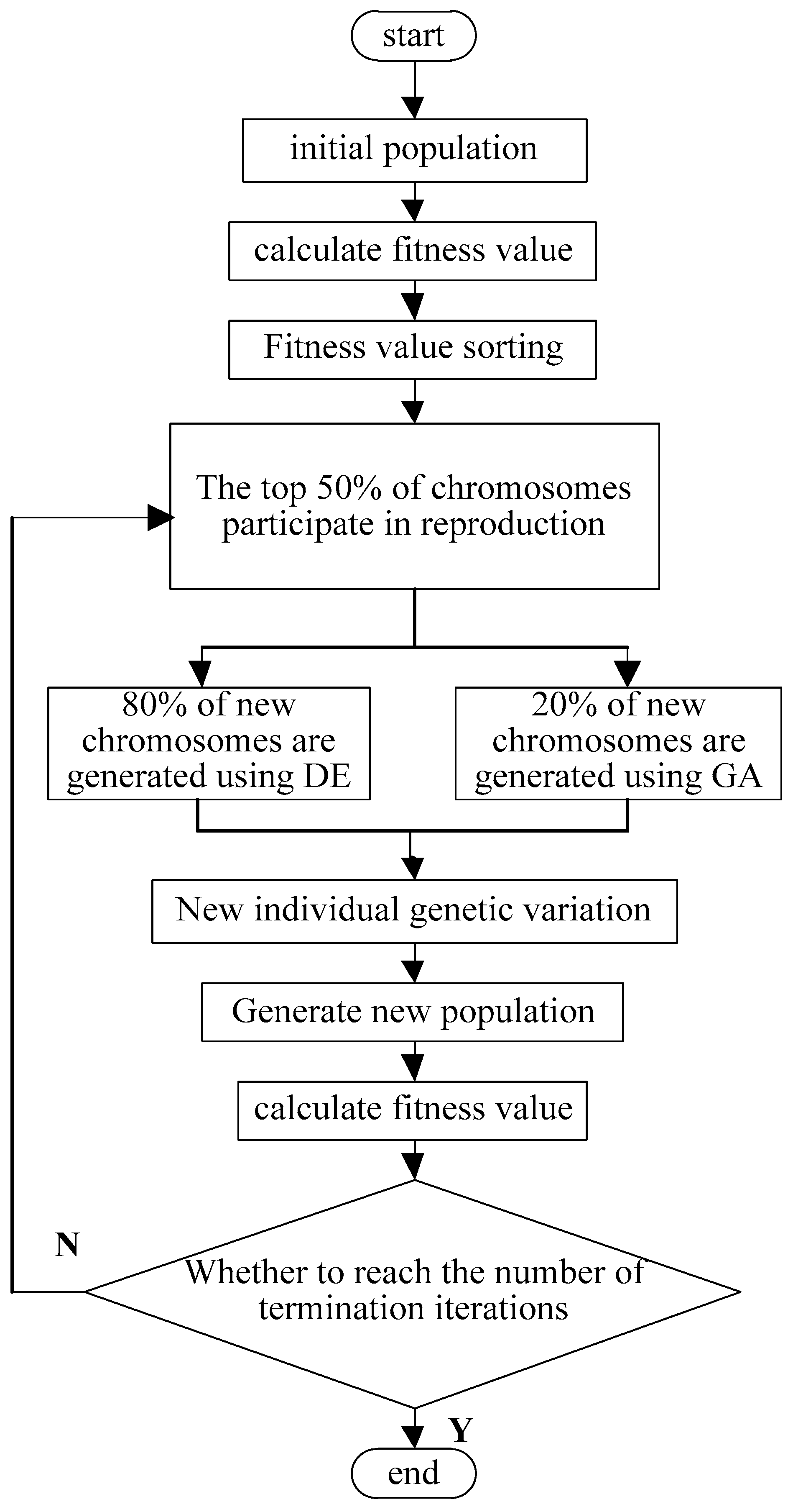
To generate a favorable label placement, a suitable optimization algorithm should be adopted to find the minimum of the highly nonlinear discrete function expressed in Equation (10). To generate an optimal label placement, a global optimization method such as the genetic algorithm (GA) is regarded as a well-known and strong method. The GA generates new individuals by simulating natural genetic recombination and evolution, allowing chromosomes to generate new individuals through selection, crossover, and mutation operators. While GA enables the minimization of highly nonlinear objective functions, the poor efficiency and convergence limit the scalability of the algorithm for complex optimization of large-scale variables as in Equation (10). Moreover, in solving the objective function for label placement, two individuals with high fitness values are likely to have dissimilar label placement, and the recombination may result in offspring with poor performance. On the other hand, differential evolution (DE), as another type of evolutionary strategy, evolves based on the difference of gene positions between chromosomes, in which the mutation, selection and crossover operations are all based on vectors and new individuals are derived from the linear combination of multiple parents [32]. As DE always accepts improved vectors without any other tournament selection, it allows a fast convergence to the minimum. When the DE is applied to solve the discrete optimization problem, it is discretized to give the discrete differential evolution algorithm (DDE).

The literature survey indicates that hybrid evolutionary algorithms are a popular strategy for solving complex optimization problems. To efficiently solve the discrete problem of automatic cartographic label placement, we propose the discrete differential evolution and genetic algorithm (DDEGA), which combines the strengths of GA and DDE to form a superior algorithm. A flowchart of a generic DDEGA framework for solving optimization problems is shown in Figure 2. DDEGA uses the framework of GA that is suitable for discrete variables in our problem and is hybridized with the mutation scheme of DDE to improve the optimization efficiency. The resulting hybrid algorithm inherits the ability of GA for selecting the fittest individuals while allowing the generation of better chromosomes in differential evolution. In successive iterations of the DDEGA, the memory and group search ability of DDE are used to adaptively adjust the internal search direction to the minimum.

3.2. DDEGA Process

3.2.1. Initial Population Generation and Coding

We define $N$ as the number of features which need to be labeled for the target map. For the MGFLP problem, $N$ is the number of the point, line and area features. As mentioned in Section 2.1, the candidate locations for line and area feature are continuous variables, thus the searching scheme that is used for line and area features becomes computationally intractable. To make the problem tractable, we take 8 candidate positions for each feature on the map. That is, the number of candidate positions for line and area features (the $k$ value in the Section 2.1) is the same as the number of candidate positions for point features. Generation of the initial population is not a trivial process. We adopted a random initialization method for generating the initial populations for DDEGA. The random initial populations can theoretically be spread throughout the search space. To create initial populations that allow sufficient search of the solution space, we use a real number to represent the candidate positions. According to the priority of each candidate position, the eight candidate positions of each feature are coded by real numbers 0–7, where a smaller number means a higher priority for the candidate position. A candidate position is randomly selected among the eight candidate positions for each graphic feature, and the selected positions of all features are combined into a set $G\left(N\right)$. According to the coding rule and gene position, a set of solutions for an initial population are generated. We also define $M$ as the size of population, in other words, by repeating the production steps according to the rules described above, a population of a certain size can be generated. Using the above scheme, we convert the set of label locations to the chromosomal genome, which results in a population representing various graphic features that is operable by the DDEGA.

3.2.2. Fitness Function

The quality metric formulated in Section 2.2 is used as the fitness function of the algorithm, which should be as low as possible. In Equation (10), the assignment of the $W_j$ directly affects the value of $S$. According to adjustment after trial experiments, the weights of each factor were finally set to $W_1=0.5$, $W_2=0.3$, $W_3=0.15$, and $W_4=0.05$.

3.2.3. Selection Operation

In the DDEGA framework, the selection operation of GA is preserved, which includes a selection operation and a copy operation. The combination of a selection operator and a copy operator benefits the generation of new individuals to increase the search possibility, and ensures the evolution of high-fitness individuals. The operator is a mathematical selection strategy, which is used to preserve or discard the individuals. Different selection strategies lead to different selection pressures. Selecting a high-pressure operator can reduce the diversity of the population faster than an operator with less pressure, and the evolution of some individuals dominates the population. However, at the same time, it will lead to premature convergence to suboptimal solutions, limiting the search ability of the population. Selecting a small pressure operator can maintain the diversity of the population and increase the probability of convergence to the global optimal solution, but the convergence speed of the algorithm is slow. In the DDEGA algorithm, the chromosomes are arranged in order of their fitness value. The top 50% of the chromosomes are selected and participate in the next generation of reproduction. This selection strategy not only ensures the diversity of the population, but also that the convergence speed of the algorithm is not too slow. The other option is equivalent to the copy operation, which is to produce the next generation of the population. The copy operation selects the best individuals from the parents to remain in the next generation. In this paper, the elite retention method is adopted for the copying operation. Individual with the highest fitness are selected from the previous generation of populations to be retained in the next generation. Applying this operation to each generation ensures the evolution of optimal individuals.

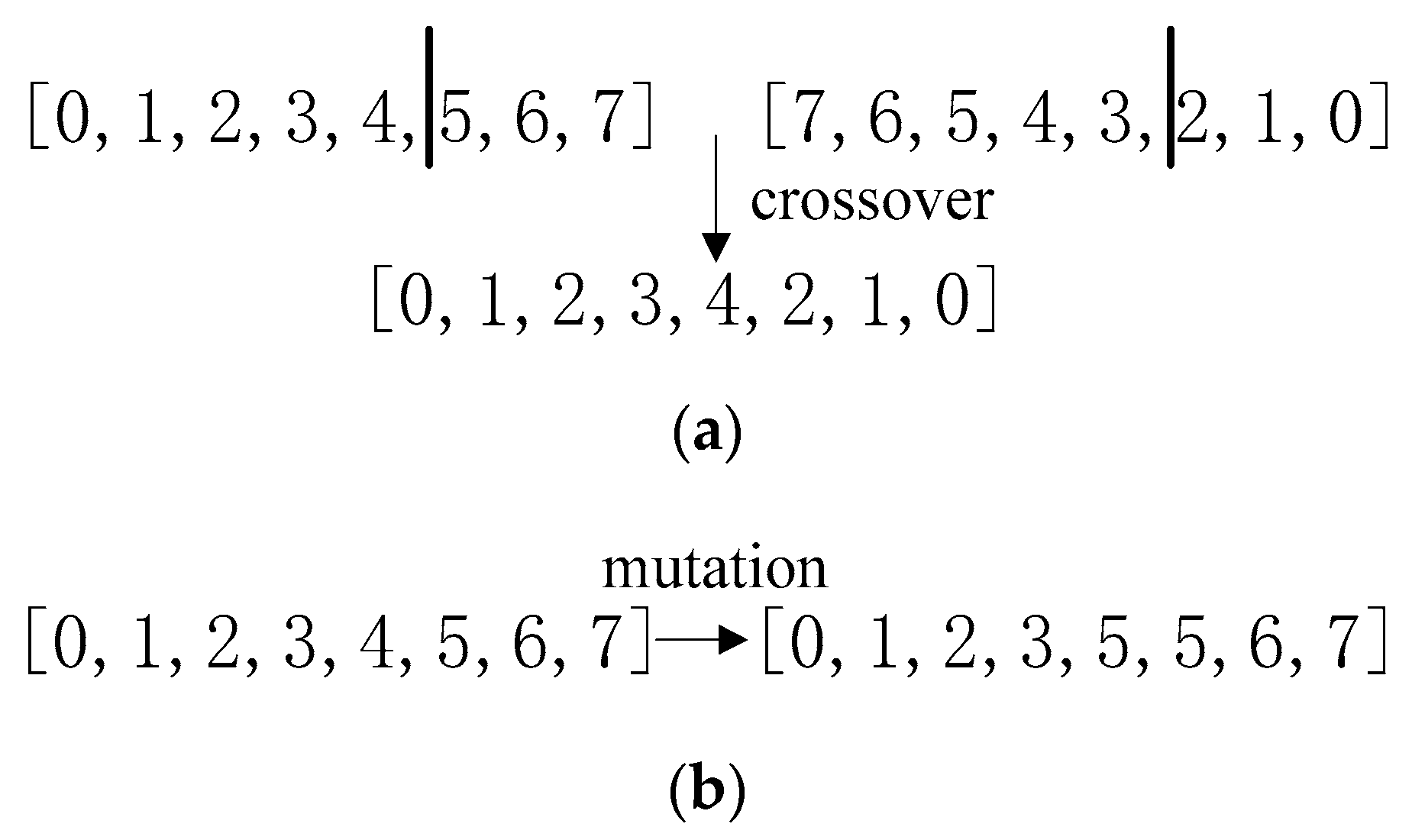
3.2.4. Variation and Crossover

The hybrid method of DDEGA combines the individual breeding method of DDE and the chromosome cross variant method of GA to generate a new population by the mutation and crossover operators of GA and DDE. The crossover operator is a single point intersection of GA, and can increase the diversity of the population and expand the search space. As shown in Figure 3a, the crossover operator refers to random extraction of two sets of chromosomes from the population, which is combined according to the crossing rule to make a new chromosome.

The main purpose of the mutation operator is to add new gene combination to increase the population diversity without destroying the superior genes of individuals with high fitness. Therefore, mutations mainly target individuals with lower fitness. The mutation operator randomly changes one gene or portions of genes of a chromosome. For example, the mutation of a gene position of a chromosome is decremented, as shown in Figure 3b.

The core of the DDE is to use a differential strategy for the mutation operation, thereby improving the ability of the algorithm to search for the global solution. Under sufficient conditions for applying the variation operator, we define $x_i\left(t\right)$ as the $i$th individual in the $t$th generation. Three different vectors, $x_{r1}\left(t\right)$, $x_{r2}\left(t\right)$ and $x_{r3}\left(t\right)$, are randomly selected from population. The difference between two of the vectors is scaled by a scaling factor $F$ and added to the third vector to obtain a new variation vector $V_i\left(t\right)$:

$$V_i\left(t\right)=x_{r1}\left(t\right)+F\left(x_{r2}\left(t\right)-x_{r3}\left(t\right)\right)$$

(11)

The vector $V_i\left(t\right)$ that undergoes the differential mutation operation may be outside the search space, and it needs to be repaired. According to the coding rules of chromosomes, gene values range from 0 to 7. When one of the gene values of the newly generated chromosome is out of range, the vector is adjusted to make it operable using a repair operator defined as follows:

$$v_i\left(t\right)=\{\begin{array}{c}0,if{v}_i\left(t\right)<0\\ 7,if{v}_i\left(t\right)>7\end{array}$$

(12)

To improve the diversity of the population, the DDE introduces the discrete hybrid operator $\mu { }_i\left(t\right)$. The hybrid operator in other evolutionary algorithms is based on multiple exchange vectors from the reference vector in the parent. In contrast, the hybrid operator in the DDE operates with the reference vector and the repaired vector. Therefore, the repaired vector $v_i\left(t\right)$ and the corresponding reference vector $h_i\left(t\right)$ in the population are selected according to a certain hybridization probability $C_r$ to increase the diversity of the population. The larger is the value of $C_r$, the greater is the possibility of hybridization. The equation is expressed as:

$${\mu }_i\left(t\right)=\{\begin{array}{l}{v}_i\left(t\right),ifrand\left[0,1\right]<C_r\\ h_i\left(t\right),otherwise\end{array}$$

(13)

4. Experimental Results

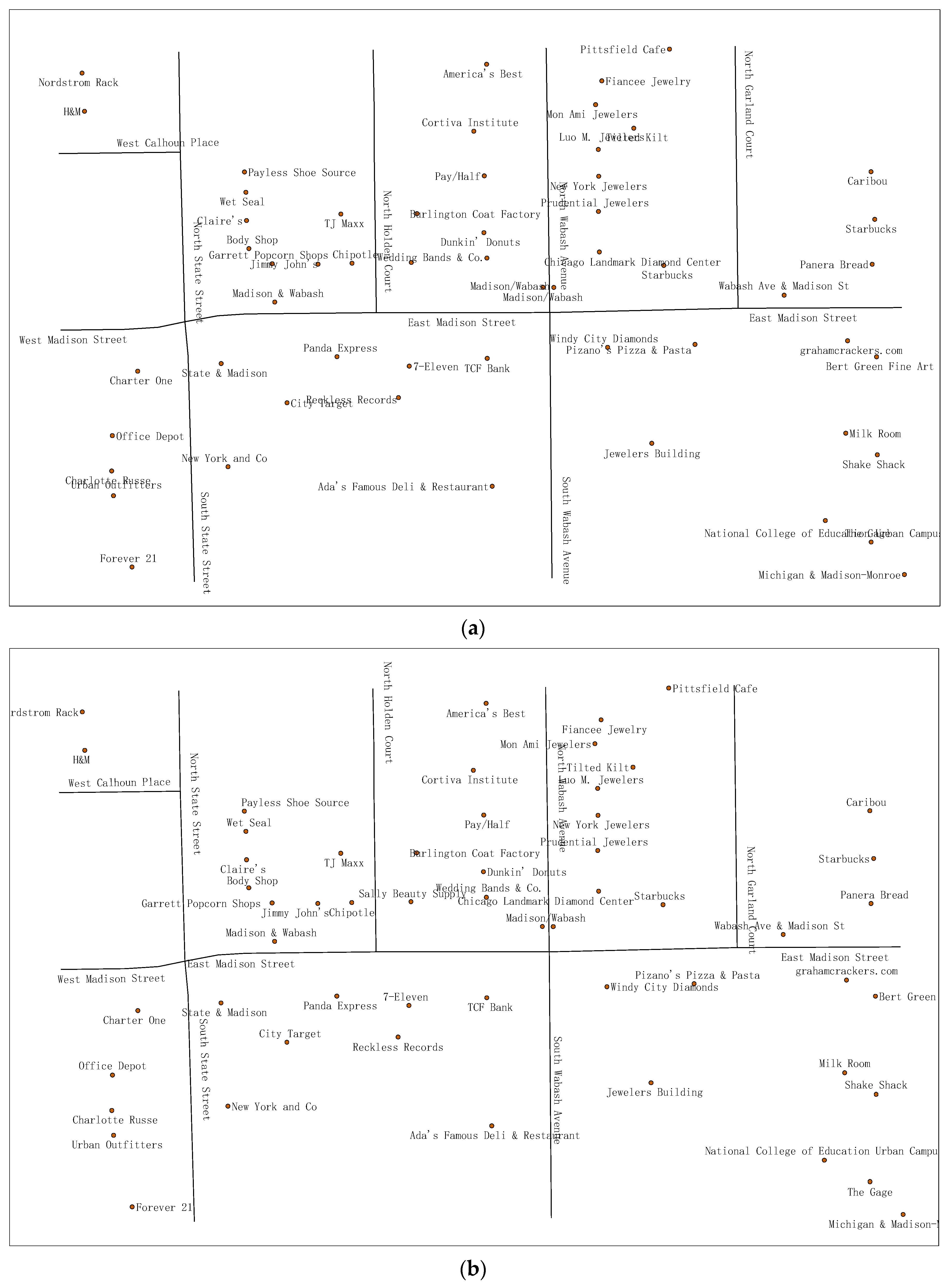
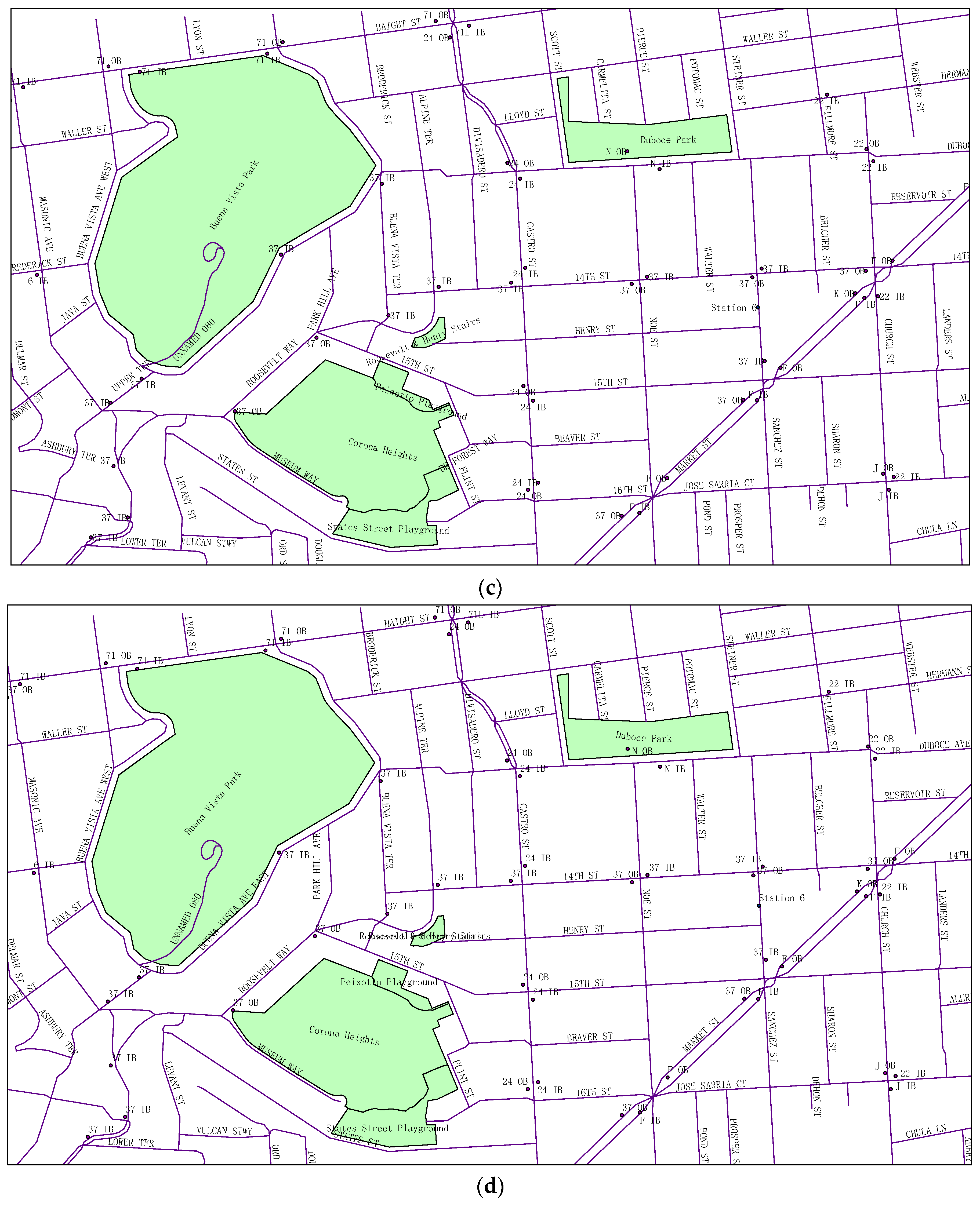
4.1. Label Placement Experiment Using DDEGA

As evidence that the hybrid DDEGA has the potential to generate cartographically plausible labeling, we present a selection of sample maps with 56 point features and 10 line features. The sample maps exhibit the ability of the DDEGA to improve the tradeoffs in the evaluation criteria for geographical features. The DDEGA algorithm was implemented in Python scripts under ArcGIS 10.2 to generate automatic label placement. In our implementation, the probability of variation F, hybridization probability $C_r$ and genetic variation were set to 0.5, 0.8 and 0.1, respectively.

Figure 4 shows a simple application of the label placement. The results generated proved to be clear and readable and show the effectiveness of the DDEGA in label placement. Initially, labels were placed in random locations (Figure 4a). At this moment, the quality of labeling was not promising; there were many label conflicts and the labels were quite cluttered. After the algorithm iterated 50 times, as shown in Figure 4b, most of the labels were suitably placed, but some overlaps still existed. Figure 4c shows the optimal solution generated by the algorithm. Most label conflicts were resolved and the relationship between the labels and features was relatively tight.

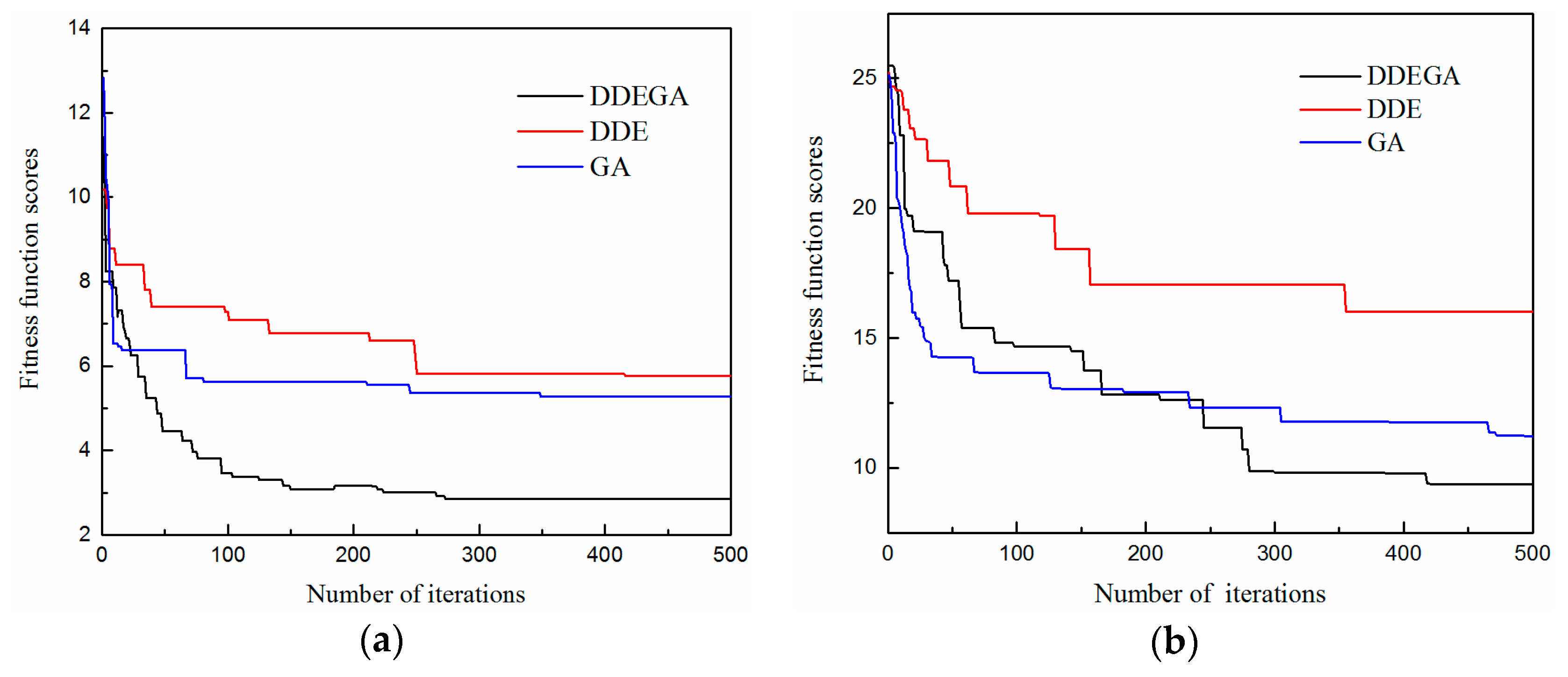
4.2. Experimental Analysis

For improving the efficiency of the GA for the MGFLP problem, this paper proposes a hybrid DDEGA algorithm that combines the advantage of GA and DDE. The efficiency and effectiveness of the DDEGA to solve the MGFLP problem were verified by using two case studies. The first case study was a map of the administrative region, cities and main roads of Washington State, which contains 15 point features, 17 line features and 39 area features. All features were labeled with eight candidate positions. The second case study included streets, parks and bus stations near Buena Vista Park in San Francisco with 163 features consisting of 73 point features, 84 line features and 6 area features.

To further verify the practicality of our proposed solution using the DDEGA algorithm in actual production, we not only compared the result of DDEGA with GA and DDE, but also compared it with the optimal result of Maplex Label Engine. The Maplex Label Engine is a smart labeling module provided by ArcGIS Development that provides advanced label layout and conflict detection methods to help users improve the quality of labeling on the map [33]. Maplex has two options for label placement, quick and optimization. Quick is the default option for providing a quick preview of the label placement. Optimization uses a more complex placement calculation to place the labels in a better final position. In this study, the results of the optimization option were used for the experiment.

Figure 5 and Figure 6 show the results from DDEGA, GA, DDE, and Maplex for the two case studies. Comparison of the results for the two examples indicates that the labels generated by DDEGA proved to be good and agree with the label rules for features better than GA and DDA. The labels generated by DDEGA were clearer than the labels generated by the other two algorithms. In the two case studies, DDEGA basically eliminated the label conflict, the label-feature conflict was smaller than the other two algorithms, and the position of labels was more reasonable, indicating that the most appropriate labeling result was produced by DDEGA.

The result generated by the DDEGA was also compared with Maplex. In the labeling result generated by Maplex, the positions of some labels were more reasonable, but there were some obvious label-feature conflicts. As shown in Figure 5d, an overlap conflict was detected between the label “Bremerton” and the point feature symbol named “Bellevue”. As shown in Figure 6d, the label “24 OB” and the point feature symbol named “71L IB” overlapped each other, and there were other instances of label conflicts. The labels generated by DDEGA did not exhibit this problem, thus we conclude that the DDEGA algorithm yielded a better result than Maplex.

The convergence of the fitness function of the three algorithms is presented for the two case studies in Figure 7. In our experiment, the DDEGA displayed the best fitness scores for the optimal solution of label placement. Comparing the two convergence figures, we observed that new individuals were continuously generated through evolution of the population in DDEGA, and the algorithm converged quickly. When the population matured, it converged and gave the optimal solution. The early convergence of the GA was fast but the algorithm fell into a local minimum within 50 generations. It was difficult to produce new individuals with high fitness to obtain an optimal result in the end. The DDE exhibited continuous convergence; however, due to the large randomness of generation, the speed of convergence was relatively slow.

By comparing the labeling results and the characteristics of the convergence function of the three algorithms, experimental results indicate that the DDEGA yielded better results than GA and DDE. We can conclude that DDEGA enabled an effective and efficient solution of MGFLP problem compared to GA and DE, indicating that our method could further improve solutions for the MGFLP problem.

5. Conclusions and Future Work

In this paper, we describe a label placement problem in which various types of geographical features are jointly labeled within a unified framework. We propose a hybrid algorithm combining discrete differential evolution and genetic algorithm (DDEGA) to search for an optimal solution. The graphic features (e.g., point, line, and area features) are labeled simultaneously. By the conversion of the set of label locations to a chromosomal genome, the population becomes operable by the DDEGA. This algorithm can achieve label placement and promote better decision-making for the multiple graphic feature label placement (MGFLP) problem. To evaluate the quality of label placement, the relationship between all graphic features and their labels is fully considered in a weighted metric for four evaluation factors. The experimental results show that our quality metric has a good performance for assessing the clarity of information on a map.

The results of the experimental annotations in multiple cases demonstrate the efficiency and effectiveness of DDEGA. The results of label placement and convergence function of different algorithms in case studies show that the performance and abilities of DDEGA are superior to GA, DDE and Maplex. Therefore, DDEGA can be considered as a new practical method to solve the MGFLP problem.

Future research will focus on adding more labeling rules for the MGFLP problem to make the positions of labels more reasonable. In this paper, we only use some of the most basic rules (e.g., label conflict, label-feature conflict, label non-ambiguity, and label priority) to determine the positions of the labels. Many secondary rules should also be considered, such as that places on the shoreline of oceans or other bodies of water should have their labels entirely on the water [34], labels should be placed wholly on the land or ocean [3], and others. Full consideration of these rules would ensure the proper representation of labels for many cartographic applications. Therefore, it is of great interest to add more labeling requirements to our algorithm for solving the MGFLP problem.

References

1. Schrijver, A. Combinatorial Optimization: Polyhedra and Efficiency; Springer: Berlin/Heidelberg Germany, 2004; Volume 27, pp. 153–159. [Google Scholar]
2. Yoeli, P. The Logic of Automated Map Lettering. Cartogr. J. 1972, 9, 99–108. [Google Scholar] [CrossRef]
3. Imhof, E. Positioning Names on Maps. Am. Cartogr. 1975, 2, 128–144. [Google Scholar] [CrossRef]
4. Marks, J.; Shieber, S. The Computational Complexity of Cartographic Label Placement; Technical Report TR-05-91; Harvard University: Cambridge, MA, USA, 1991; pp. 5–91. [Google Scholar]
5. Formann, M.; Wagner, F. A packing problem with applications to lettering of maps. In Proceedings of the Seventh Annual Symposium on Computational Geometry, North Conway, NH, USA, 10–12 June 1991; pp. 281–288. [Google Scholar]
6. Zoraster, S. Practical Results Using Simulated Annealing for Point Feature Label Placement. Cartogr. Geogr. Inf. Syst. 1997, 24, 228–238. [Google Scholar] [CrossRef]
7. Mauri, G.; Ribeiro, G.M.; Lorena, L.A.N. A new mathematical model and a Lagrangean decomposition for the point-feature cartographic label placement problem. Comput. Oper. Res. 2010, 37, 2164–2172. [Google Scholar] [CrossRef]
8. Marín, A.; Pelegrín, M. Towards unambiguous map labeling-Integer programming approach and heuristic algorithm. Expert Syst. Appl. 2018, 98, 221–241. [Google Scholar] [CrossRef]
9. Gomes, S.P.; Ribeiro, G.M.; Lorena, L.A.N. Dispersion for the point-feature cartographic label placement problem. Expert Syst. Appl. 2013, 40, 5878–5883. [Google Scholar] [CrossRef]
10. Cravo, G.L.; Ribeiro, G.M.; Lorena, L.A.N. A greedy randomized adaptive search procedure for the point-feature cartographic label placement. Comput. Geosci. 2008, 34, 373–386. [Google Scholar] [CrossRef]
11. Verner, O.V.; Wainwright, R.L.; Schoenefeld, D.A. Placing text labels on maps and diagrams using genetic algorithms with masking. INFORMS J. Comput. 1997, 9, 266–275. [Google Scholar] [CrossRef]
12. Azamathulla, H.M.; Wu, F.C.; Ab Ghani, A.; Narulkar, S.M.; Zakaria, N.A.; Chang, C.K. Comparison between genetic algorithm and linear programming approach for real time operation. J. Hydro-Environ. Res. 2008, 2, 172–181. [Google Scholar] [CrossRef]
13. Li, L.; Zhang, H.; Zhu, H.; Kuai, X.; Hu, W. A Labeling Model Based on the Region of Movability for Point-Feature Label Placement. ISPRS Int. J. Geo-Inf. 2016, 5, 159. [Google Scholar] [CrossRef]
14. Yamamoto, M.; Lorena, L.A.N. A Constructive Genetic Approach to Point-Feature Cartographic Label Placement. Metaheuristics Prog. Real Probl. Solv. 2005, 32, 287–302. [Google Scholar] [CrossRef]
15. Gomes, S.P.; Lorena, L.A.N.; Ribeiro, G.M. A Constructive Genetic Algorithm for Discrete Dispersion on Point Feature Cartographic Label Placement Problems. Geogr. Anal. 2016, 48, 43–58. [Google Scholar] [CrossRef]
16. Doerschler, J.S.; Freeman, H. A rule-based system for dense-map name placement. Commun. ACM 1992, 35, 68–79. [Google Scholar] [CrossRef]
17. Wolff, A.; Knipping, L.; Kreveld, M.v.; Strijk, T.; Agarwal, P.K. A Simple and Efficient Algorithm for High-Quality Line Labeling; Technical Report UU-CS-2001-44; Department of Computer Science, Utrecht University: Utrecht, The Netherlands, 1997; Volume 11, pp. 146–150. [Google Scholar]
18. Sun, S.; Zhao, H.; Fang, J.; Cheng, Z.; Zhao, Y. A pratical Method for Line Labeling. In Proceedings of the 18th International Conference on Geoinformatics: GIScience in Change, Peking University, Beijing, China, 18–20 June 2010; pp. 18–20. [Google Scholar]
19. Wu, C.; Ding, Y.; Zhou, X.; Lu, G. A grid algorithm suitable for line and area feature label placement. Environ. Earth Sci. 2016, 75, 1368. [Google Scholar] [CrossRef]
20. Pfefferkorn, C.; Burr, D.; Harrison, D.; Heckman, B. A Cartographic Expert System. In Proceedings of the Seventh International Symposium on Autocarto, Falls Church, VA, USA, 11–14 March 1985; pp. 399–407. [Google Scholar]
21. Ahn, J.; Freeman, H. A Program for Automatic Name Placement. Cartogr. Int. J. Geogr. Inf. Geovis. 1984, 21, 101–109. [Google Scholar] [CrossRef]
22. Rylov, M.; Reimer, A. A Practical Algorithm for the External Annotation of Area Features. Cartogr. J. 2016, 54, 61–76. [Google Scholar] [CrossRef]
23. Edmondson, S.; Christensen, J.; Marks, J.; Shieber, S. A General Cartographic Labelling Algorithm. Cartogr. Int. J. Geogr. Inf. Geovis. 1996, 33, 13–24. [Google Scholar] [CrossRef] [Green Version]
24. Kakoulis, K.G.; Tollis, I.G. A unified approach to automatic label placement. Int. J. Comput. Geom. Appl. 2003, 13, 23–59. [Google Scholar] [CrossRef]
25. Zhang, Q.; Harrie, L. Placing Text and Icon Labels Simultaneously: A Real-Time Method. Cartogr. Geogr. Inf. Sci. 2006, 33, 53–64. [Google Scholar] [CrossRef]
26. Price, K.V.; Storn, R.M.; Lampinen, J.A. Differential Evolution: A Practical Approach to Global Optimization; Springer: Berlin/Heidelberg Germany, 2005; Volume 141. [Google Scholar]
27. Jia, L.Y.; He, J.X.; Zhang, C.; Gong, W.Y. Differential evolution with controlled search direction. J. Cent. South Univ. 2012, 19, 3516–3523. [Google Scholar] [CrossRef]
28. Ebinger, L.R.; Goulette, A.M. Automated Name Palcement in a Non-Interactive Environment. Available online: https://pdfs.semanticscholar.org/114f/ab94f3b7c96cf1992cf66f171828ed310966.pdf (accessed on 12 April 2019).
29. Klau, G.W.; Mutzel, P. Optimal labeling of point features in rectangular labeling models. Math. Program. 2003, 94, 435–458. [Google Scholar] [CrossRef]
30. Ribeiro, G.M.; Lorena, L.A.N. Column generation approach for the point-feature cartographic label placement problem. J. Comb. Optim. 2008, 15, 147–164. [Google Scholar] [CrossRef]
31. Alvim, A.C.F.; Taillard, É.D. POPMUSIC for the point feature label placement problem. Eur. J. Oper. Res. 2009, 192, 396–413. [Google Scholar] [CrossRef]
32. Storn, R.; Price, K. Differential Evolution–A Simple and Efficient Heuristic for global Optimization over Continuous Spaces. J. Glob. Optim. 1997, 11, 341–359. [Google Scholar] [CrossRef]
33. What Is the Maplex Label Engine? Available online: http://desktop.arcgis.com/zh-cn/arcmap/10.3/map/working-with-text/what-is-maplex-.htm (accessed on 10 April 2019).
34. Gomarasca, M.A. Elements of Cartography; Springer: Dordrecht, The Netherlands, 2009; pp. 19–77. [Google Scholar] [CrossRef]
Figure 1. (a) A candidate-position model of a point feature; (b) a candidate-position model of a line feature; and (c) a candidate-position model of an area feature.
Ijgi 08 00237 g001
Figure 2. Flowchart for the DDEGA.
Ijgi 08 00237 g002
Figure 3. The crossover and mutation operator of GA: (a) crossover; and (b) mutation.
Ijgi 08 00237 g003
Figure 4. The progression of label placement with the DDEGA algorithm: (a) the initial random labeling of a generated map; (b) the map with label placement after 50 iterations of the algorithm; and (c) the final labeling of the map.
Ijgi 08 00237 g004aIjgi 08 00237 g004b
Figure 5. The map of Washington State with labels generated by four approaches: (a) GA; (b) DDE; (c) DDEGA; and (d) Maplex.
Ijgi 08 00237 g005aIjgi 08 00237 g005b
Figure 6. Map of near Buena Vista Park in San Francisco with labels generated by four approaches: (a) GA; (b) DDE; (c) DDEGA; and (d) Maplex.
Ijgi 08 00237 g006aIjgi 08 00237 g006b
Figure 7. (a) Convergence of each algorithm for the first case study; and (b) convergence of each algorithm for the second case study.
Ijgi 08 00237 g007