Identifying Modes of Driving Railway Trains from GPS Trajectory Data: An Ensemble Classifier-Based Approach

Abstract
1. Introduction
1.1. Background
1.2. Related Works
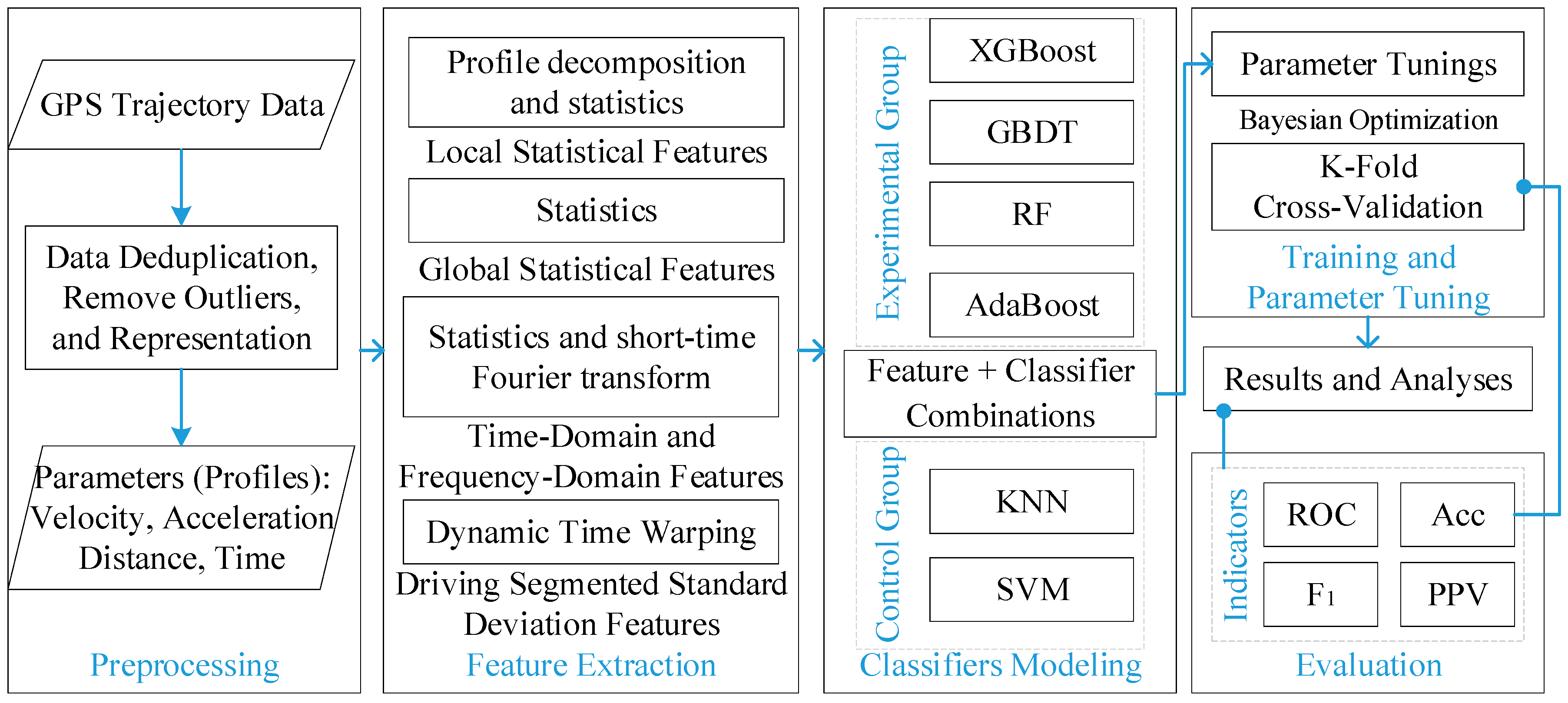
2. Methodologies
2.1. Preprocessing
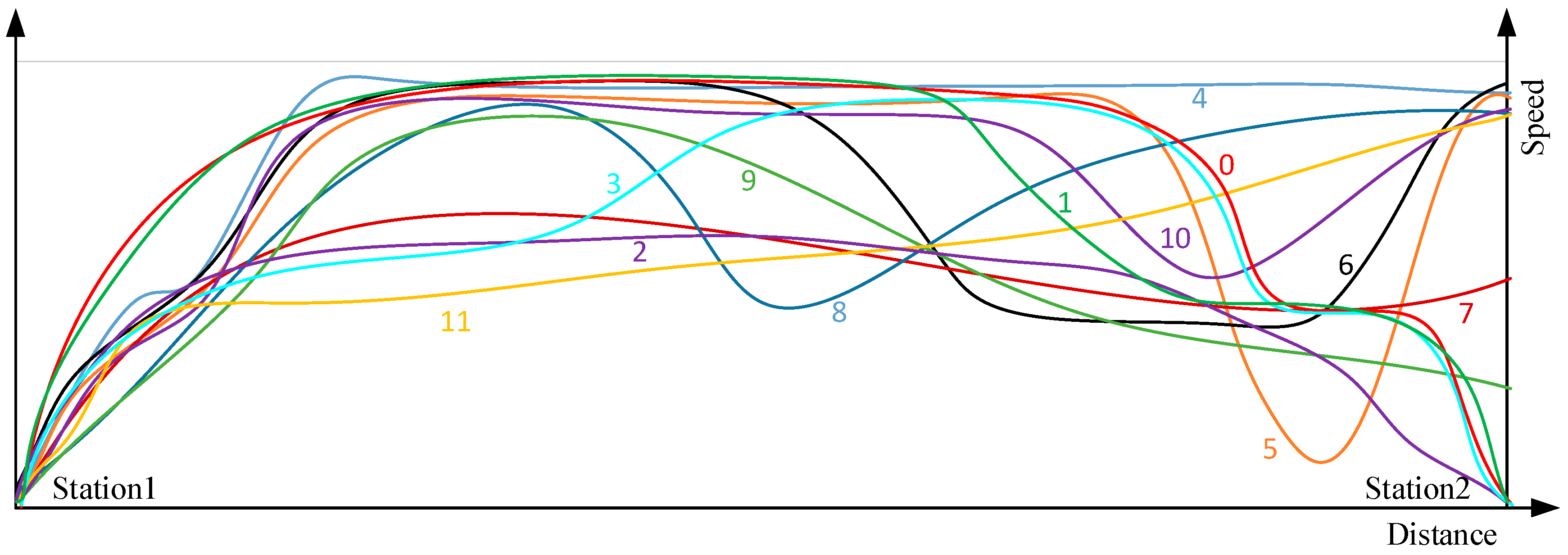
2.1.1. Modes of Driving Railway Train
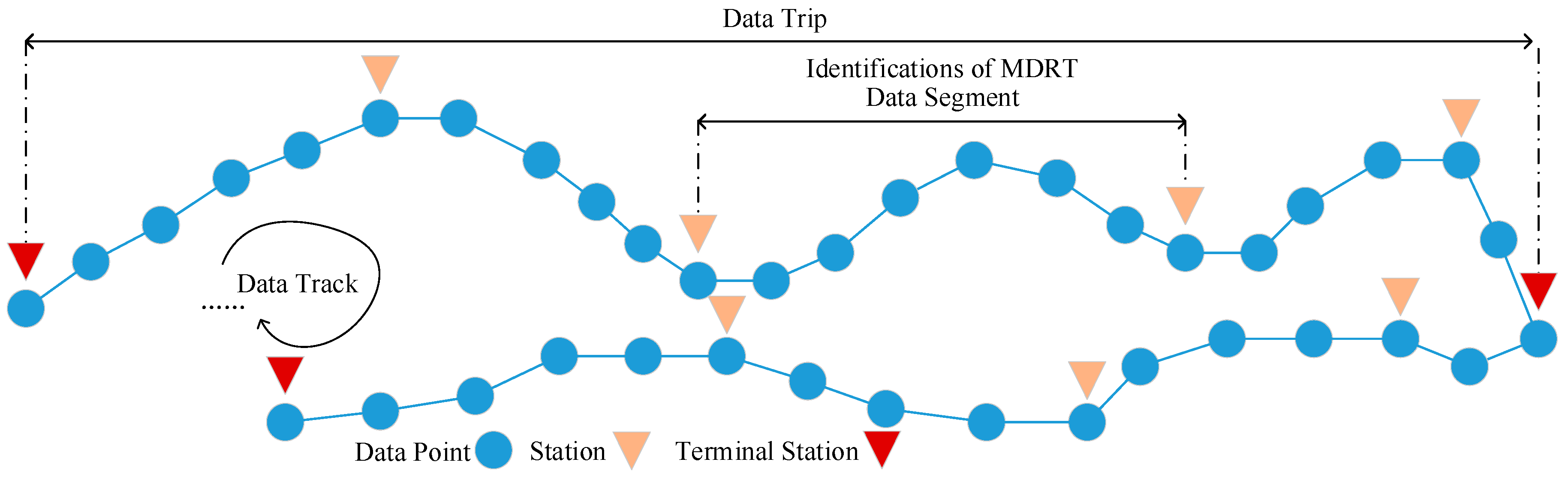
2.1.2. Representation and Segments of Trajectory Data
2.2. Feature Extraction
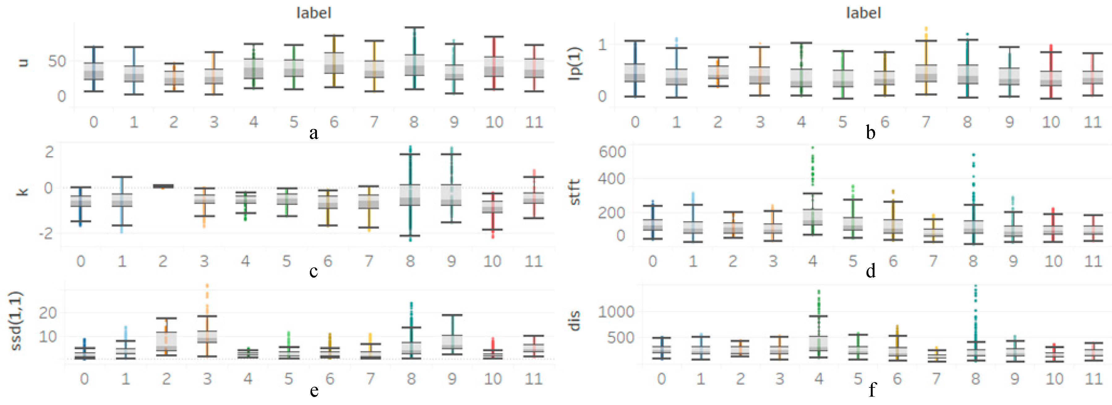
2.2.1. Classical Features
2.2.2. Driving Segmented Standard Deviation Features (DSSDF)
2.2.3. Features Summary
2.3. Classifiers Modeling and Parameter Tuning
2.3.1. Classifiers Modeling
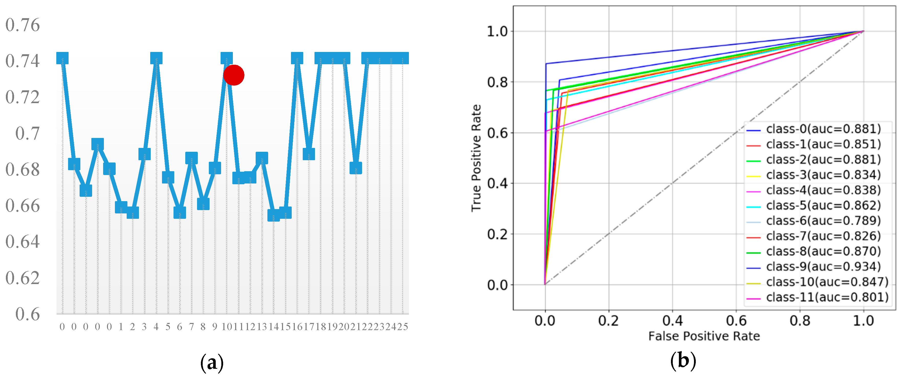
2.3.2. Parameter Tuning
2.4. Evaluation Methods and Cross-Validation
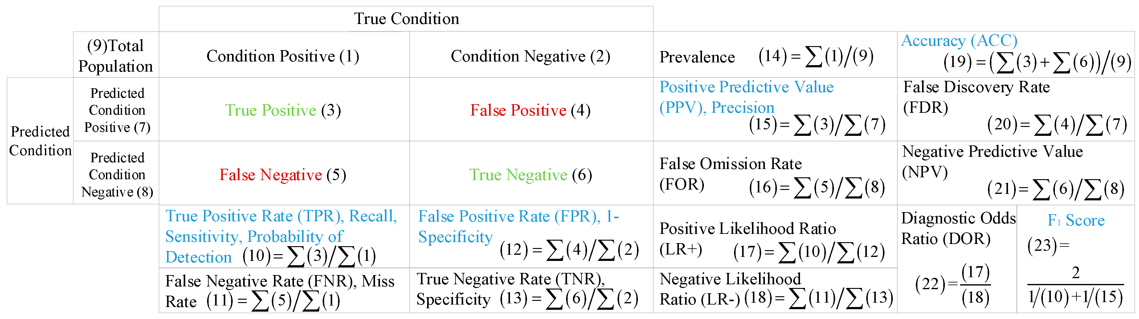
2.4.1. Evaluation Indicators
2.4.2. K-Fold Cross-Validation
3. Results and Discussion
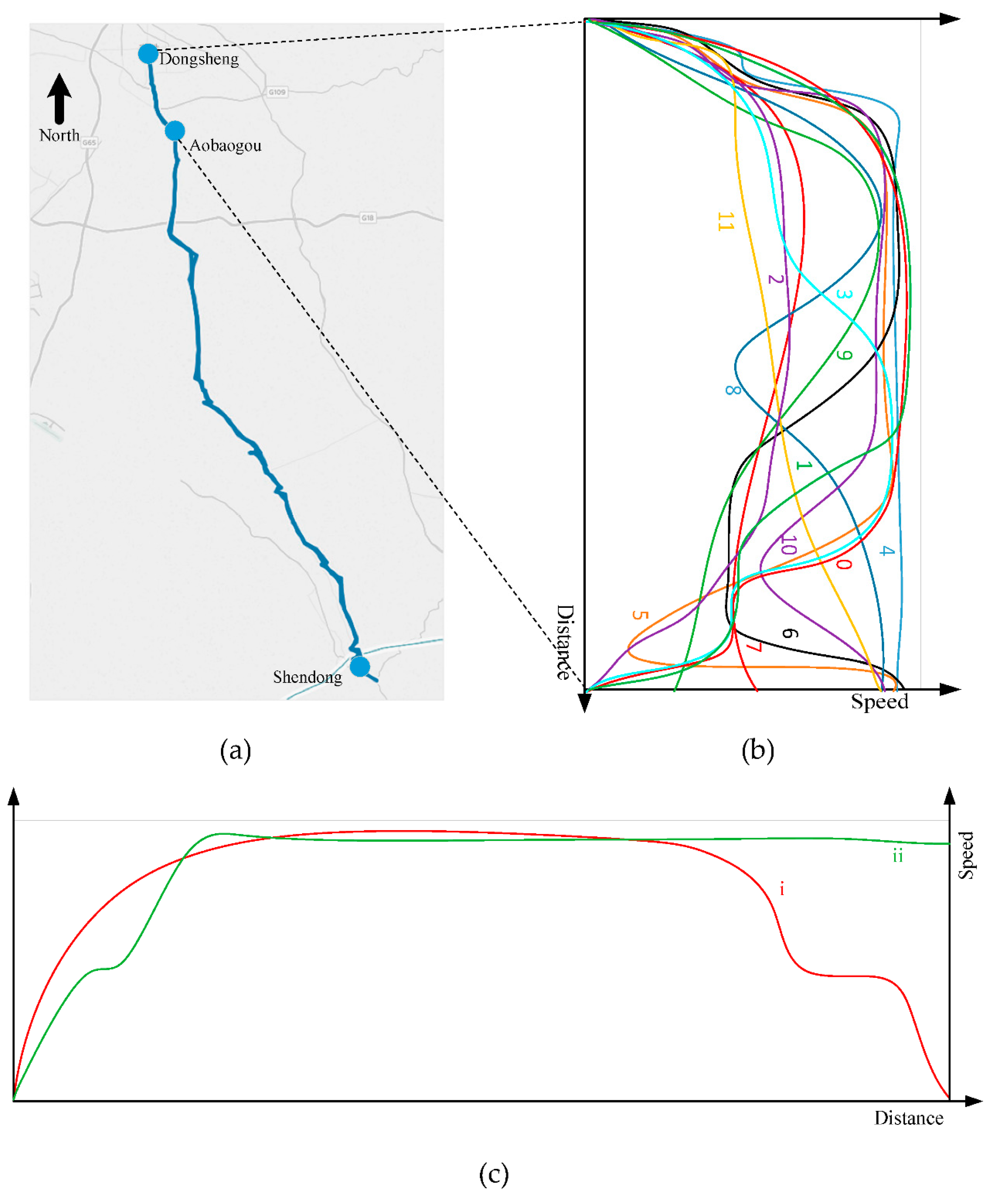
3.1. Experiment Data
3.2. Experiment Scheme
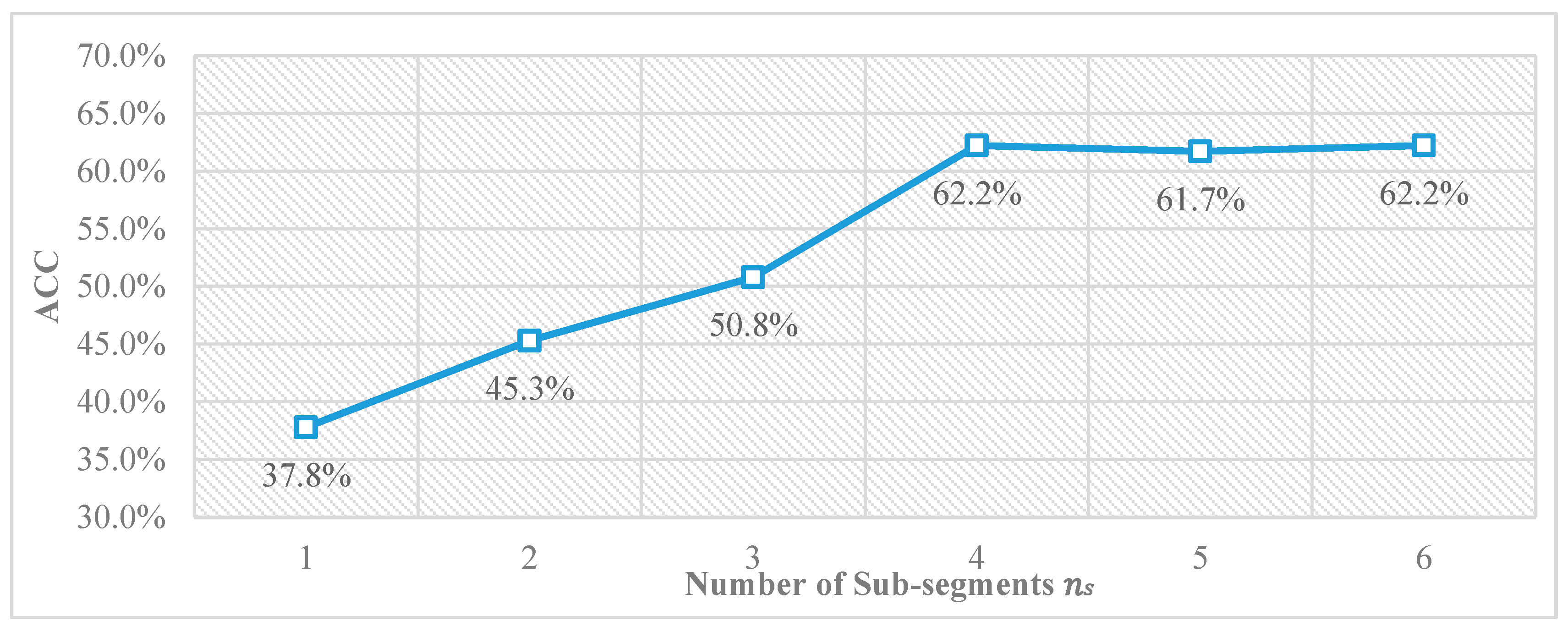
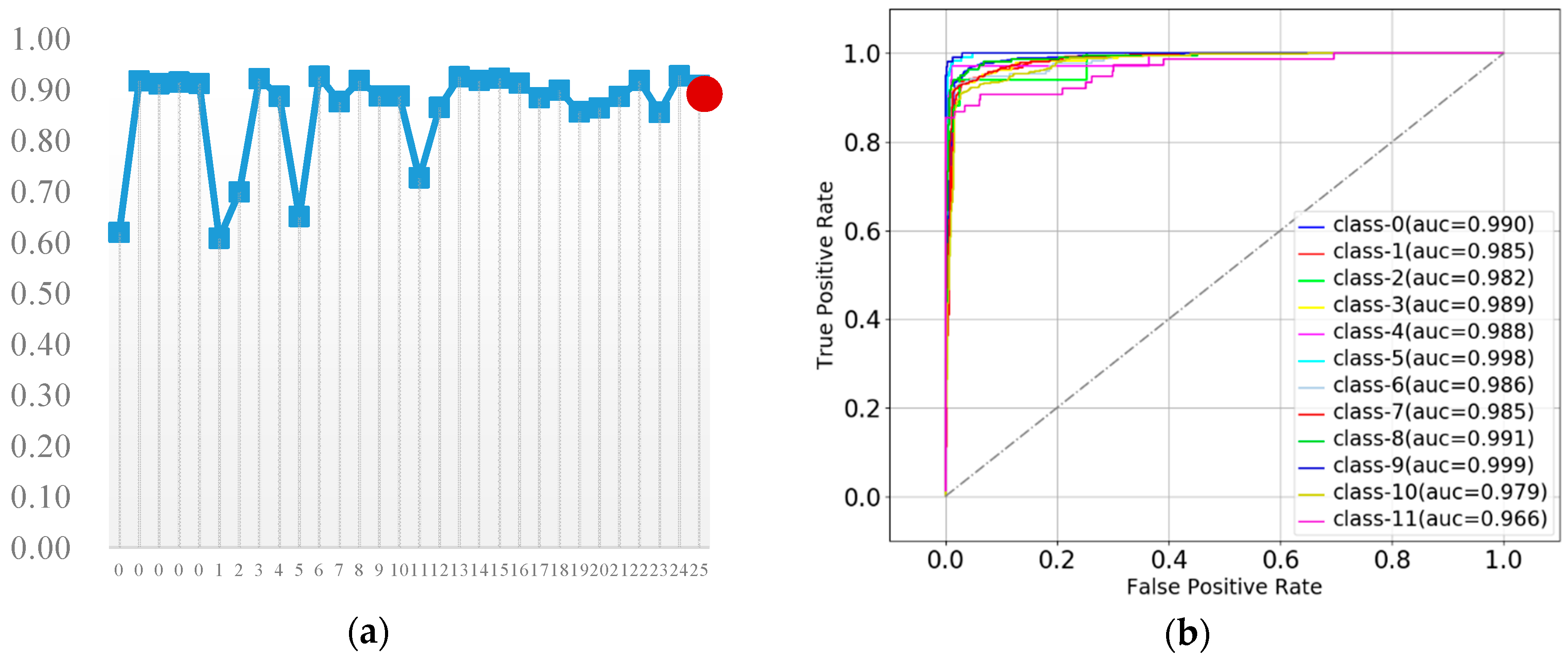
3.3. Determination the Optimal Value of
3.4. Classifiers Performance Evaluations
3.4.1. K-Nearest Neighbor
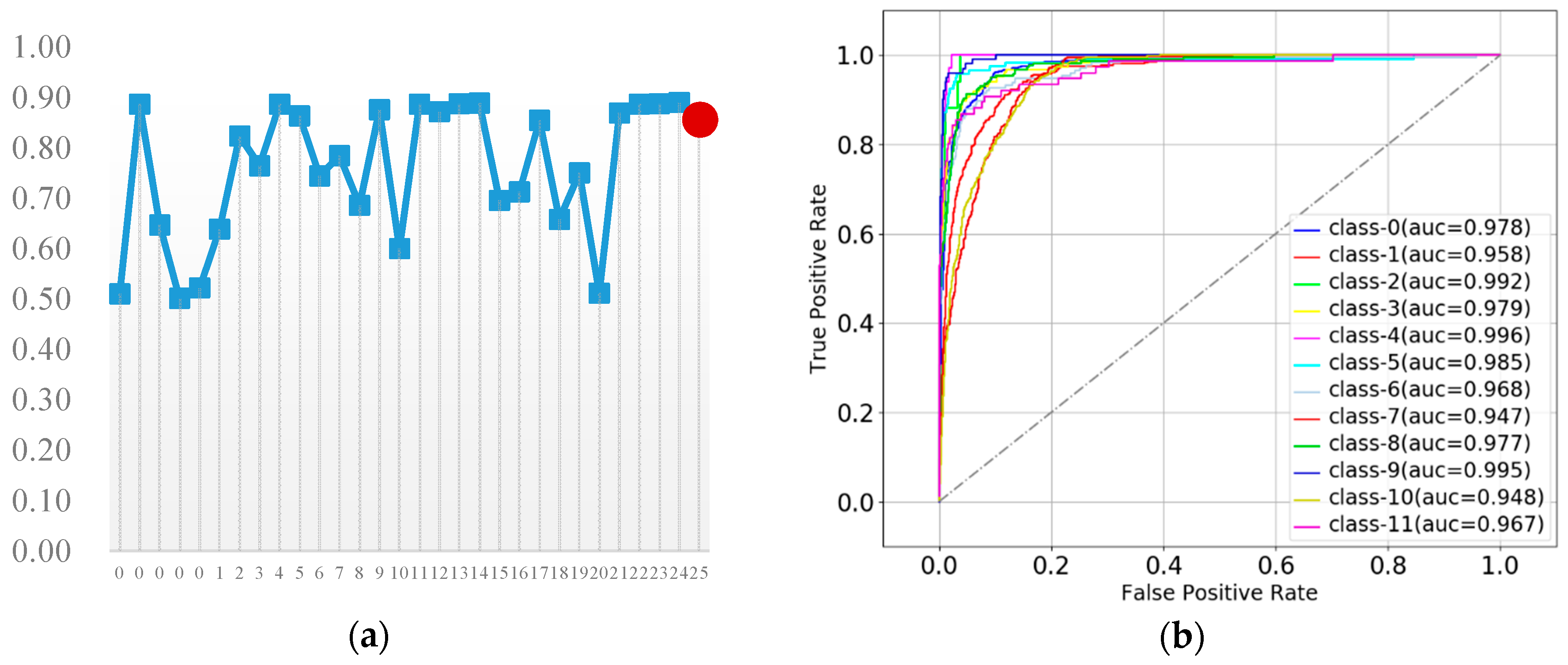
3.4.2. Support Vector Machines
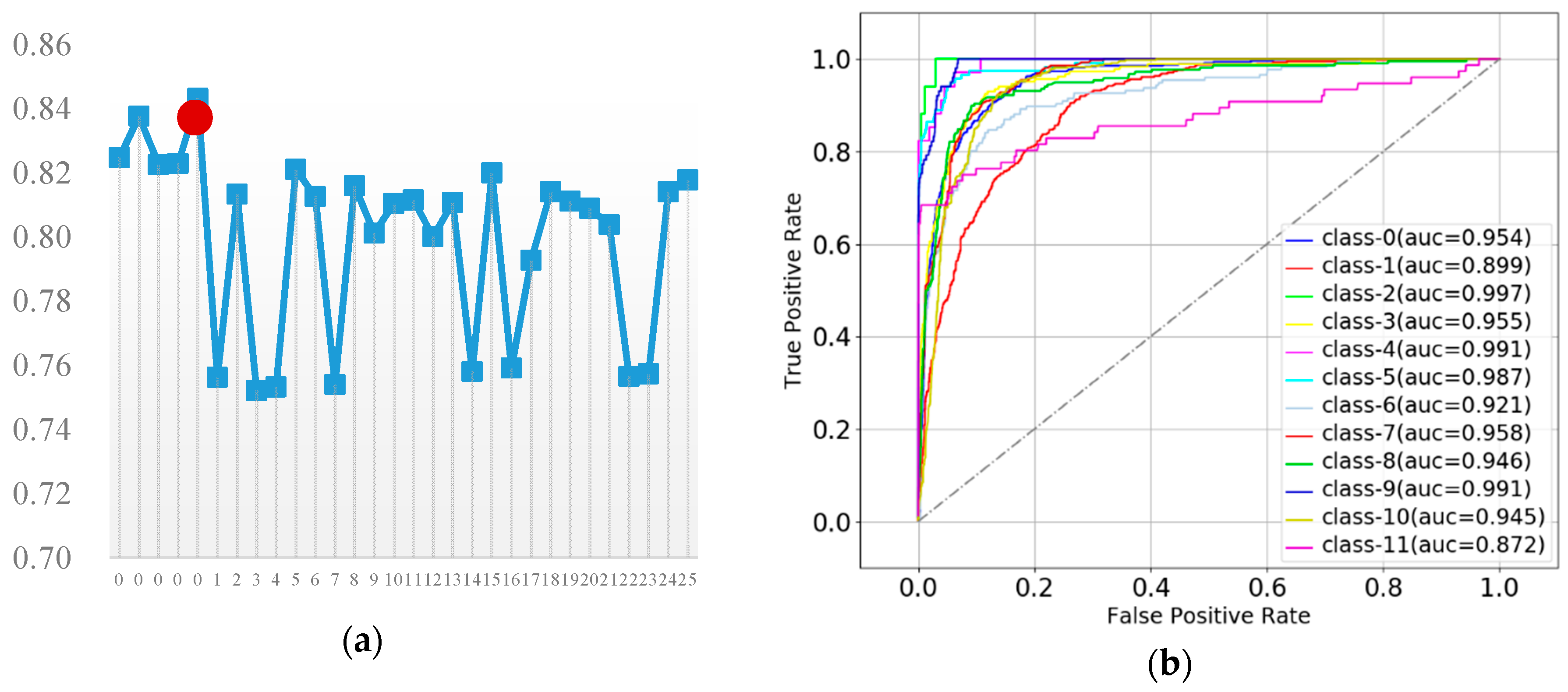
3.4.3. AbaBoost
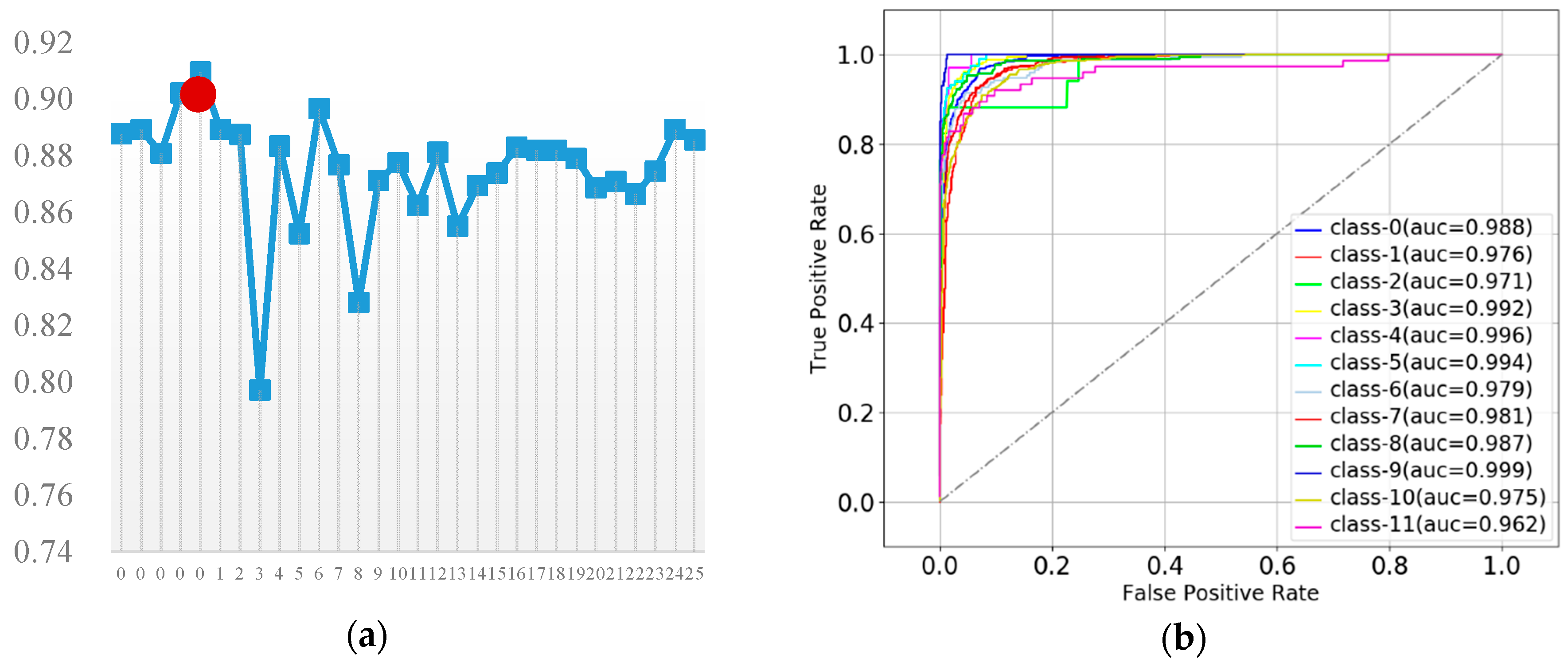
3.4.4. Random Forest
3.4.5. Gradient Boosting Decision Tree
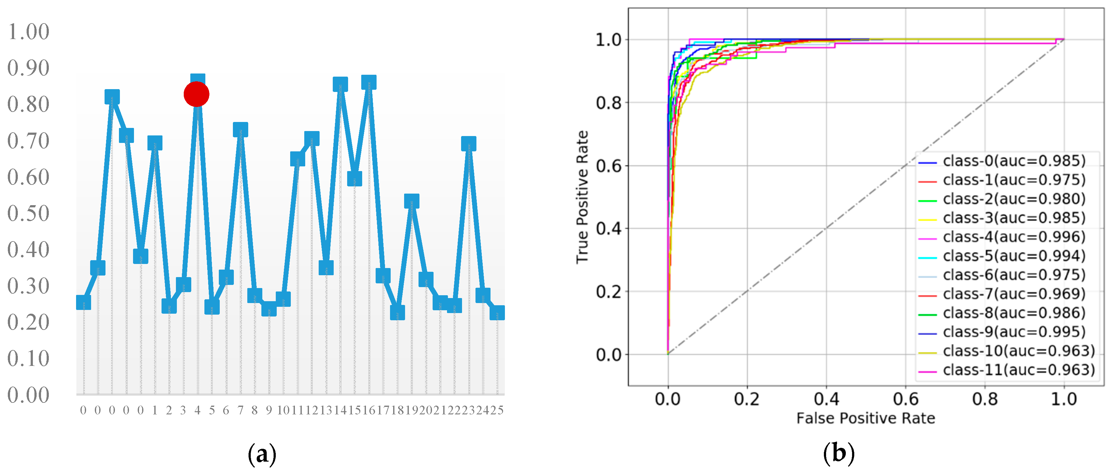
3.4.6. Extreme Gradient Boosting
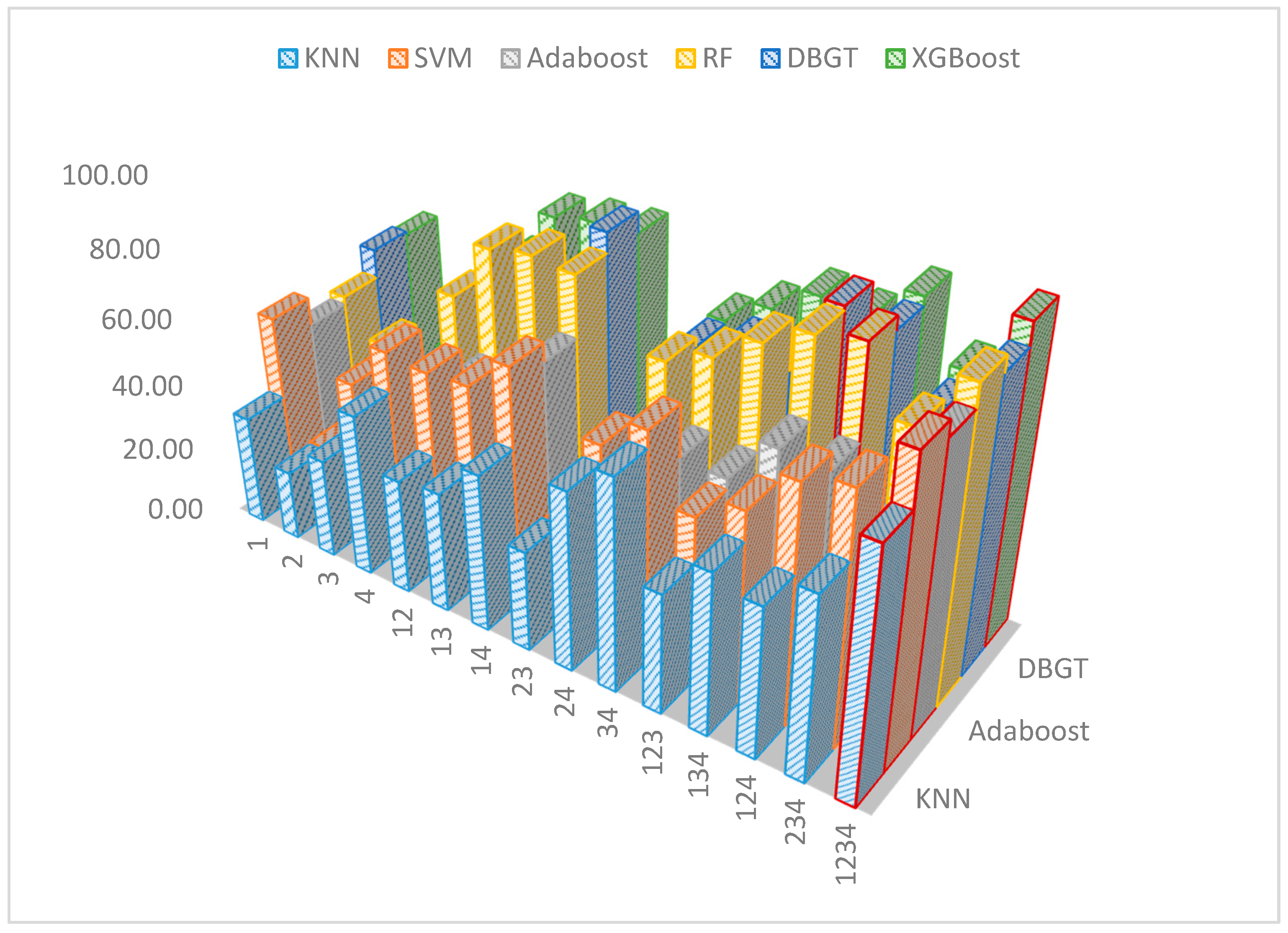
3.5. The Comparison of Features and Classifiers
4. Conclusions
Author Contributions
Funding
Conflicts of Interest
References
- Chen, J.; Zhang, X.; Cai, H.; Zheng, Y. A monitoring data mining based approach to measuring and correcting timetable parameters. Procedia Soc. Behav. Sci. 2012, 43, 644–652. [Google Scholar] [CrossRef]
- Wang, J.; Zhang, X.; Yi, Z.; Chen, J. Method for the measurement and correction of train diagram parameters based on monitoring data mining. China Railw. Sci. 2011, 32, 117–121. [Google Scholar]
- Longo, G.; Medeossi, G.; Nash, A. Estimating train motion using detailed sensor data. In Proceedings of the Transportation Research Board 91st Annual Meeting, Washington, DC, USA, 22–26 January 2012; pp. 1–6. [Google Scholar]
- Zhou, L.; Tong, L.; Chen, J.; Tang, J.; Zhou, X. Joint optimization of high-speed train timetables and speed profiles: A unified modeling approach using space-time-speed grid networks. Transp. Res. Part B Methodol. 2017, 97, 157–181. [Google Scholar] [CrossRef]
- Bešinović, N. Integrated Capacity Assessment and Timetabling Models for Dense Railway Networks; Netherlands TRAIL Research School: Delft, The Netherlands, 2017. [Google Scholar]
- Bešinović, N.; Goverde, R.M.P.; Quaglietta, E.; Roberti, R. An integrated micro–macro approach to robust railway timetabling. Transp. Res. Part B Methodol. 2016, 87, 14–32. [Google Scholar] [CrossRef]
- Fabris, S.D.; Longo, G.; Medeossi, G. Automated analysis of train event recorder data to improve micro-simulation models. In Proceedings of the COMPRAIL 2010 Conference, Beijing, China, 31 August–2 September 2010; pp. 575–583. [Google Scholar]
- Powell, J.P.; Palacín, R. Driving Style for Ertms Level 2 and Conventional Lineside Signalling: An Exploratory Study; ResearchGate: Berlin, Germany, 2016. [Google Scholar]
- Medeossi, G.; Longo, G.; Fabris, S.D. A method for using stochastic blocking times to improve timetable planning. J. Rail Transp. Plan. Manag. 2011, 1, 1–13. [Google Scholar] [CrossRef]
- Goverde, R.M.P.; Daamen, W.; Hansen, I.A. Automatic identification of route conflict occurrences and their consequences. In Computers in Railways XI; WIT Press: Southampton, UK, 2008; pp. 473–482. [Google Scholar]
- Albrecht, T.; Goverde, R.M.P.; Weeda, V.A.; Luipen, J.V. Reconstruction of train trajectories from track occupation data to determine the effects of a driver information system. In Proceedings of the COMPRAIL 2006 Conference, Prague, Czech Republic, 31 August–2 September 2006; pp. 207–216. [Google Scholar]
- Dodge, S.; Weibel, R.; Forootan, E. Revealing the physics of movement: Comparing the similarity of movement characteristics of different types of moving objects. Comput. Environ. Urban Syst. 2009, 33, 419–434. [Google Scholar] [CrossRef]
- Schuessler, N.; Axhausen, K.W. Processing GPS Raw Data without Additional Information; Transportation Research Board: Washington, DC, USA, 2008. [Google Scholar]
- Zheng, Y.; Liu, L.; Wang, L.; Xie, X. Learning transportation mode from raw gps data for geographic applications on the web. In Proceedings of the International Conference on World Wide Web (WWW 2008), Beijing, China, 21–25 April 2008; pp. 247–256. [Google Scholar]
- Wagner, D.P. Lexington Area Travel Data Collection Test: GPS for Personal Travel Surveys; Elsevier: Amsterdam, The Netherlands, 1997. [Google Scholar]
- Yalamanchili, L.; Pendyala, R.; Prabaharan, N.; Chakravarthy, P. Analysis of global positioning system-based data collection methods for capturing multistop trip-chaining behavior. Transp. Res. Rec. J. Transp. Res. Board 1999, 1660, 58–65. [Google Scholar] [CrossRef]
- Draijer, G.; Kalfs, N.; Perdok, J. Global positioning system as data collection method for travel research. Opt. Express 2000, 1719, 147–153. [Google Scholar] [CrossRef]
- Wolf, J.L. Using GPS Data Loggers to Replace Travel Diaries in the Collection of Travel Data. Ph.D. Thesis, School of Civil and Environmental Engineering, Georgia Institute of Technology, Atlanta, GA, USA, 2000. [Google Scholar]
- Stenneth, L.; Wolfson, O.; Yu, P.S.; Xu, B. Transportation mode detection using mobile phones and gis information. In Proceedings of the ACM Sigspatial International Symposium on Advances in Geographic Information Systems (ACM-GIS 2011), Chicago, IL, USA, 1–4 November 2011; pp. 54–63. [Google Scholar]
- Gonzalez, P.A.; Weinstein, J.S.; Barbeau, S.J.; Labrador, M.A.; Winters, P.L.; Georggi, N.L.; Perez, R. Automating mode detection using neural networks and assisted gps data collected using gps-enabled mobile phones. In Proceedings of the 15th World Congress on Intelligent Transport Systems and ITS America’s 2008 Annual Meeting, New York, NY, USA, 16–20 November 2008. [Google Scholar]
- Xiao, Z.; Wang, Y.; Fu, K.; Wu, F. Identifying different transportation modes from trajectory data using tree-based ensemble classifiers. ISPRS Int. J. Geo-Inf. 2017, 6, 57. [Google Scholar] [CrossRef]
- Patterson, D.J.; Liao, L.; Fox, D.; Kautz, H. Inferring High-Level Behavior from Low-Level Sensors; Springer: Berlin, Germany, 2003; pp. 73–89. [Google Scholar]
- Lin, L.; Fox, D.; Kautz, H. Learning and inferring transportation routines. In Proceedings of the 19th National Conference on Artifical Intelligence, San Jose, CA, USA, 25–29 July 2004; pp. 348–353. [Google Scholar]
- Zheng, Y.; Li, Q.; Chen, Y.; Xie, X.; Ma, W.Y. Understanding mobility based on gps data. In Proceedings of the 10th International Conference on Ubiquitous Computing, Seoul, Korea, 21–24 September 2008; pp. 312–321. [Google Scholar]
- Reddy, S.; Min, M.; Burke, J.; Estrin, D.; Hansen, M.; Srivastava, M. Using mobile phones to determine transportation modes. ACM Trans. Sensor Netw. 2010, 6, 13. [Google Scholar] [CrossRef]
- Elhoushi, M.; Georgy, J.; Noureldin, A.; Korenberg, M. Online motion mode recognition for portable navigation using low-cost sensors. Navigation 2016, 62, 273–290. [Google Scholar] [CrossRef]
- Widhalm, P.; Nitsche, P.; Brändle, N. Transport mode detection with realistic smartphone sensor data. In Proceedings of the 2012 21st International Conference on Pattern Recognition (ICPR), Tsukuba, Japan, 11–15 November 2012; pp. 573–576. [Google Scholar]
- Das, R.D.; Winter, S. Detecting urban transport modes using a hybrid knowledge driven framework from gps trajectory. Int. J. Geo-Inf. 2016, 5, 207. [Google Scholar] [CrossRef]
- Mardia, K.V.; Jupp, P.E. Directional Statistics; Wiley: Chichester, UK, 2000. [Google Scholar]
- Deng, H.; Runger, G.; Tuv, E.; Vladimir, M. A time series forest for classification and feature extraction. Inf. Sci. 2013, 239, 142–153. [Google Scholar] [CrossRef]
- Zhang, J.; Wang, Y.; Zhao, W. An improved hybrid method for enhanced road feature selection in map generalization. Int. J. Geo-Inf. 2017, 6, 196. [Google Scholar] [CrossRef]
- Qian, H.; Lu, Y. Simplifying gps trajectory data with enhanced spatial-temporal constraints. Int. J. Geo-Inf. 2017, 6, 329. [Google Scholar] [CrossRef]
- Ma, C.; Zhang, Y.; Wang, A.; Wang, Y.; Chen, G. Traffic command gesture recognition for virtual urban scenes based on a spatiotemporal convolution neural network. ISPRS Int. J. Geo-Inf. 2018, 7, 37. [Google Scholar] [CrossRef]
- Jahangiri, A.; Rakha, H.A. Applying machine learning techniques to transportation mode recognition using mobile phone sensor data. IEEE Trans. Intell. Transp. Syst. 2015, 16, 2406–2417. [Google Scholar] [CrossRef]
- Bagnall, A.; Lines, J.; Bostrom, A.; Large, J.; Keogh, E. The great time series classification bake off: A review and experimental evaluation of recent algorithmic advances. Data Min. Knowl. Discov. 2017, 31, 606–660. [Google Scholar] [CrossRef]
- Feng, T.; Timmermans, H.J.P. Transportation mode recognition using gps and accelerometer data. Tramsp. Res. Part C Emerg. Technol. 2013, 37, 118–130. [Google Scholar] [CrossRef]
- Xiao, G.; Juan, Z.; Zhang, C. Travel mode detection based on gps track data and bayesian networks. Comput. Environ. Urban Syst. 2015, 54, 14–22. [Google Scholar] [CrossRef]
- Bishop, C.M. Pattern Recognition and Machine Learning (Information Science and Statistics); Springer: New York, NY, USA, 2006; p. 049901. [Google Scholar]
- Nielsen, D. Tree Boosting with Xgboost—Why Does Xgboost win “ Every” Machine Learning Competition? Master’s Thesis, Norwegian University of Science and Technology, Trondheim, Norway, 2016. [Google Scholar]
- Chen, T.; Guestrin, C. Xgboost: A scalable tree boosting system. In Proceedings of the ACM SIGKDD International Conference on Knowledge Discovery and Data Mining, San Francisco, CA, USA, 13–17 August 2016; pp. 785–794. [Google Scholar]
- Guo, L.; Ge, P.S.; Zhang, M.H.; Li, L.H.; Zhao, Y.B. Pedestrian detection for intelligent transportation systems combining adaboost algorithm and support vector machine. Expert Syst. Appl. 2012, 39, 4274–4286. [Google Scholar] [CrossRef]
- Kowsari, T.; Beauchemin, S.S.; Cho, J. Real-time vehicle detection and tracking using stereo vision and multi-view adaboost. In Proceedings of the International IEEE Conference on Intelligent Transportation Systems, Washington, DC, USA, 5–7 October 2011; pp. 1255–1260. [Google Scholar]
- Khammari, A.; Nashashibi, F.; Abramson, Y.; Laurgeau, C. Vehicle detection combining gradient analysis and adaboost classification. In Proceedings of the International IEEE Conference on Intelligent Transportation Systems, Vienna, Austria, 16–16 September 2005; pp. 66–71. [Google Scholar]
- Stopher, P.; Jiang, Q.; Fitzgerald, C. Processing gps data from travel surveys. In Proceedings of the 2nd International Colloqium on the Behavioural Foundations of Integrated Land-Use and Transportation Models: Frameworks, Models and Applications, Toronto, ON, Canada, 13–14 June 2005. [Google Scholar]
- Jun, J.; Guensler, R.; Ogle, J. Smoothing methods to minimize impact of global positioning system random error on travel distance, speed, and acceleration profile estimates. Transp. Res. Rec. J. Transp. Res. Board 2006, 1972, 141–150. [Google Scholar] [CrossRef]
- Prelipcean, A.C.; Gidofalvi, G.; Susilo, Y.O. Measures of transport mode segmentation of trajectories. Int. J. Geogr. Inf. Sci. 2016, 30, 1763–1784. [Google Scholar] [CrossRef]
- Keogh, E.; Ratanamahatana, C.A. Exact indexing of dynamic time warping. Knowl. Inf. Syst. 2005, 7, 358–386. [Google Scholar] [CrossRef]
- Freund, Y.; Schapire, R.E. A decision-theoretic generalization of on-line learning and an application to boosting. In Proceedings of the European Conference on Computational Learning Theory, London, UK, 13–15 March 1995; pp. 23–37. [Google Scholar]
- Freund, Y.; Schapire, R.E. Experiments with a new boosting algorithm. In Proceedings of the Thirteenth International Conference on International Conference on Machine Learning, Bari, Italy, 3–6 July 1996; pp. 148–156. [Google Scholar]
- Liaw, A.; Wiener, M. Classification and regression by randomforest. R News 2002, 23, 18–22. [Google Scholar]
- Friedman, J.H. Greedy function approximation: A gradient boosting machine. Ann. Stat. 2001, 29, 1189–1232. [Google Scholar] [CrossRef]
- Friedman, J.H. Stochastic gradient boosting. Comput. Stat. Data Anal. 2002, 38, 367–378. [Google Scholar] [CrossRef]
- Cover, T.; Hart, P. Nearest neighbor pattern classification. IEEE Trans.Inf. Theory 2002, 13, 21–27. [Google Scholar] [CrossRef]
- Cortes, C. Support vector network. Mach. Learn. 1995, 20, 273–297. [Google Scholar] [CrossRef]
- Liu, L.; Shen, B.; Wang, X. Research on Kernel Function of Support Vector Machine; Springer: Dordrecht, The Netherlands, 2014; pp. 827–834. [Google Scholar]
- Claesen, M.; Moor, B.D. Hyperparameter search in machine learning. arXiv, 2015; arXiv:1502.02127. [Google Scholar]
- Hsu, C.W. A Practical Guide to Support Vector Classification; National Taiwan University: Taibei, Taiwan, 2010; Volume 67. [Google Scholar]
- Chicco, D. Ten quick tips for machine learning in computational biology. Biodata Min. 2017, 10, 35. [Google Scholar] [CrossRef] [PubMed]
- Wang, Z.; Hutter, F.; Zoghi, M.; Matheson, D.; De Freitas, N. Bayesian optimization in a billion dimensions via random embeddings. Comput. Sci. 2016. [Google Scholar] [CrossRef]
- Bergstra, J.; Bengio, Y. Random search for hyper-parameter optimization. J. Mach. Learn. Res. 2012, 13, 281–305. [Google Scholar]
- Bergstra, J.; Bengio, Y. Algorithms for hyper-parameter optimization. In Proceedings of the International Conference on Neural Information Processing Systems, Granada, Spain, 12–15 December 2011; pp. 2546–2554. [Google Scholar]
- Hutter, F.; Hoos, H.H.; Leyton-Brown, K. Sequential model-based optimization for general algorithm configuration. In Proceedings of the International Conference on Learning and Intelligent Optimization, Rome, Italy, 17–21 January 2011; pp. 507–523. [Google Scholar]
- Thornton, C.; Hutter, F.; Hoos, H.H.; Leytonbrown, K. Auto-weka: Combined selection and hyperparameter optimization of classification algorithms. Comput. Sci. 2012, 847–855, 847–855. [Google Scholar] [CrossRef]
- Snoek, J.; Larochelle, H.; Adams, R.P. Practical bayesian optimization of machine learning algorithms. Adv. Neural Inf. Process. Syst. 2012, 4, 2951–2959. [Google Scholar]
- Chapelle, O.; Vapnik, V.; Bousquet, O.; Mukherjee, S. Choosing multiple parameters for support vector machines. Mach. Learn. 2002, 46, 131–159. [Google Scholar] [CrossRef]


| ID | G-Name (ID) 1 | Name | Notation | R 2 |
|---|---|---|---|---|
| 1 | GSF (1) | Mean | [21,29] | |
| 2 | Standard deviation | |||
| 3 | Mode | |||
| 4 | Median | |||
| 5 | Max 3 values Min 3 values | 3 | ||
| 6 | Value Range | 3 | ||
| 7 | Percentile tuple | 4 | ||
| 8 | Interquartile Range | 4 | ||
| 9 | Skewness | |||
| 10 | Kurtosis | |||
| 11 | Coefficient of variation | |||
| 12 | Autocorrelation coefficient | |||
| 13 | Stop rate | [24] | ||
| 14 | Velocity change rate | 5 | ||
| 15 | Trajectory length | |||
| 16 | LSF (2) | Mean length of each decomposition class | 6 | [12] |
| 17 | Length standard deviation of each decomposition class | 6 | ||
| 18 | Proportion of each decomposition class | 6 | ||
| 19 | Change times | 6 | ||
| 20 | TDFDF (3) | Median crossover rate | 5 | [25,26] |
| 21 | Number of peaks | 5 | ||
| 22 | Short-time Fourier transform |
| ID | Descriptors | Feature Description | Number |
|---|---|---|---|
| 1 | GSF | , , , , (3), (3), , (2), , , , , . For each parameter (2). | |
| , , . | 3 | ||
| 2 | LSF | (4), (4), (4), . For each parameter (2). | |
| 3 | TDFDF | , , . For each parameter (2). | |
| 4 | DSSDF | (). For each parameter (2). | |
| SUM |
| Classifier | Parameter Range | Notes |
|---|---|---|
| KNN | “n_neighbors”: (1, 15) | n_neighbors (int): Number of neighbors to get. |
| SVM | “C”: (0.001, 100) “gamma”: (0.0001, 0.1) | C (float): Penalty parameter C of the error term. gamma (float): Kernel coefficient for ‘rbf’, ‘poly’ and ‘sigmoid’. |
| Ada | “n_estimators”: (10, 250) “learning_rate”: (0.001, 0.1) | n_estimators (int): The maximum number of estimators at which boosting is terminated. learning_rate (float): Learning rate shrinks the contribution of each classifier by ‘learning_rate’. There is a trade-off between “learning_rate” and “n_estimators”. |
| RF | “n_estimators”: (10, 200) “min_samples_split”: (2, 15) “max_features”: (0.1, 0.999) | n_estimators (int): number of trees in the forest. min_samples_split (int or float): The minimum number (int) or percentage (float) of samples required to split an internal node. max_features (int or float): The number or percentage of features to consider when looking for the best split. |
| GBDT | “n_estimators”: (10, 250) “learning_rate”: (0.1, 0.999) “subsample”: (0.1, 0.9) | n_estimators (int): The number of boosting stages to perform. learning_rate (float): learning rate shrinks the contribution of each tree by ‘learning_rate’. subsample (float): The fraction of samples to be used for fitting the individual base learners. |
| XGBoost | “min_child_weight”: (1, 10) “colsample_bytree”: (0.1, 1) “max_depth”: (5, 10) “subsample”: (0.5, 1) “gamma”: (0, 1) “alpha”: (0, 1) “eta”: (0.001, 0.1) | min_child_weight (int): Minimum sum of instance weight (Hessian) needed in a child. colsample_bytree (float): Subsample ratio of columns when constructing each tree. max_depth (int): Maximum tree depth for base learners. subsample (float): Subsample ratio of the training instance. gamma (float): Minimum loss reduction required to make a further partition on a leaf node of the tree. alpha (float): L1 regularization term on weights eta (float): Boosting learning rate. |
| Mode ID | Trajectory Number | Mode ID | Trajectory Number |
|---|---|---|---|
| 0 | 1218 | 6 | 441 |
| 1 | 1029 | 7 | 1050 |
| 2 | 42 | 8 | 546 |
| 3 | 462 | 9 | 252 |
| 4 | 84 | 10 | 1176 |
| 5 | 294 | 11 | 189 |
| SUM | 6783 |
| I 1 | n_n(int) 2 | ACC | I 1 | n_n(int) 2 | ACC | I 1 | n_n(int) 2 | ACC |
|---|---|---|---|---|---|---|---|---|
| 0 | 5.91 (5) | 74.1% | 6 | 13.97 (13) | 65.6% | 16 | 1.69 (1) | 60.1% |
| 0 | 2.06 (2) | 68.3% | 7 | 4.76 (4) | 68.6% | 17 | 5.28 (5) | 74.1% |
| 0 | 10.50 (10) | 66.8% | 8 | 11.64 (11) | 66.1% | 18 | 5.18 (5) | 74.1% |
| 0 | 3.83 (3) | 69.4% | 9 | 6.72 (6) | 68.1% | 19 | 5.75 (5) | 74.1% |
| 0 | 7.68 (7) | 68.0% | 10 | 5.43 (5) | 74.1% | 20 | 5.74 (5) | 74.1% |
| 1 | 15.00 (15) | 65.9% | 11 | 8.41 (8) | 67.5% | 21 | 6.25 (6) | 68.1% |
| 2 | 12.83 (12) | 65.6% | 12 | 9.83 (9) | 67.5% | 22 | 5.00 (5) | 74.1% |
| 3 | 7.74 (7) | 68.0% | 13 | 4.25 (4) | 68.6% | 23 | 5.62 (5) | 74.1% |
| 4 | 1.00 (1) | 60.1% | 14 | 14.53 (14) | 65.4% | 24 | 5.18 (5) | 74.1% |
| 5 | 9.10 (9) | 67.5% | 15 | 12.23 (12) | 65.6% | 25 | 5.75 (5) | 74.1% |
| KNN | A | |||||||||||||
|---|---|---|---|---|---|---|---|---|---|---|---|---|---|---|
| 0 | 1 | 2 | 3 | 4 | 5 | 6 | 7 | 8 | 9 | 10 | 11 | PPV | ||
| P | 0 | 80.7 | 14.6 | 11.8 | 4.9 | 2.9 | 0.0 | 4.0 | 0.7 | 0.5 | 0.0 | 1.9 | 13.2 | 77.7 |
| 1 | 10.5 | 75.5 | 11.8 | 22.7 | 2.9 | 6.8 | 5.7 | 0.7 | 0.9 | 0.0 | 0.4 | 1.3 | ||
| 2 | 0.6 | 0.5 | 76.5 | 0.5 | 0.0 | 0.0 | 0.0 | 0.0 | 0.0 | 0.0 | 0.0 | 0.0 | ||
| 3 | 1.8 | 7.3 | 0.0 | 68.6 | 0.0 | 0.0 | 0.6 | 0.5 | 0.9 | 2.0 | 0.2 | 1.3 | ||
| 4 | 0.0 | 0.0 | 0.0 | 0.0 | 67.6 | 0.8 | 0.0 | 0.0 | 0.0 | 0.0 | 0.0 | 0.0 | ||
| 5 | 0.2 | 0.0 | 0.0 | 0.0 | 8.8 | 72.9 | 2.3 | 0.0 | 0.9 | 3.0 | 0.0 | 0.0 | ||
| 6 | 1.0 | 0.7 | 0.0 | 0.0 | 2.9 | 6.8 | 60.2 | 1.0 | 8.3 | 2.0 | 3.8 | 3.9 | ||
| 7 | 1.4 | 0.2 | 0.0 | 0.0 | 0.0 | 2.5 | 1.7 | 69.5 | 3.2 | 1.0 | 14.9 | 10.5 | ||
| 8 | 0.4 | 0.5 | 0.0 | 2.7 | 14.7 | 5.9 | 10.2 | 2.4 | 76.6 | 4.0 | 2.1 | 3.9 | ||
| 9 | 0.0 | 0.0 | 0.0 | 0.0 | 0.0 | 2.5 | 3.4 | 0.0 | 0.0 | 87.1 | 0.0 | 0.0 | ||
| 10 | 2.9 | 0.7 | 0.0 | 0.0 | 0.0 | 1.7 | 9.7 | 25.0 | 7.8 | 1.0 | 76.6 | 5.3 | ||
| 11 | 0.4 | 0.0 | 0.0 | 0.5 | 0.0 | 0.0 | 2.3 | 0.2 | 0.9 | 0.0 | 0.0 | 60.5 | ||
| TPR | 72.9 | F1: 74.9 | ||||||||||||
| I 1 | C | Gamma | ACC | I 1 | C | Gamma | ACC | I 1 | C | Gamma | ACC |
|---|---|---|---|---|---|---|---|---|---|---|---|
| 0 | 43.936 | 0.03 | 50.9% | 6 | 0.001 | 0.03 | 74.3% | 16 | 0.002 | 0.08 | 71.2% |
| 0 | 5.636 | 0.09 | 88.6% | 7 | 99.999 | 0.10 | 78.4% | 17 | 99.996 | 0.04 | 85.4% |
| 0 | 7.577 | 0.07 | 64.6% | 8 | 0.007 | 0.03 | 68.5% | 18 | 0.004 | 0.07 | 65.7% |
| 0 | 43.207 | 0.08 | 50.0% | 9 | 0.004 | 0.03 | 87.5% | 19 | 100.000 | 0.00 | 75.0% |
| 0 | 79.405 | 0.04 | 52.1% | 10 | 100.000 | 0.09 | 59.9% | 20 | 100.000 | 0.00 | 51.1% |
| 1 | 99.999 | 0.09 | 63.8% | 11 | 0.002 | 0.02 | 88.6% | 21 | 0.005 | 0.04 | 86.8% |
| 2 | 0.001 | 0.04 | 82.2% | 12 | 0.008 | 0.07 | 87.1% | 22 | 0.001 | 0.07 | 88.6% |
| 3 | 99.999 | 0.07 | 76.4% | 13 | 0.004 | 0.07 | 88.7% | 23 | 0.002 | 0.07 | 88.7% |
| 4 | 0.004 | 0.10 | 88.6% | 14 | 0.003 | 0.01 | 88.8% | 24 | 0.001 | 0.01 | 88.9% |
| 5 | 99.996 | 0.09 | 86.3% | 15 | 0.002 | 0.08 | 69.5% | 25 | 0.003 | 0.06 | 86.2% |
| SVM | A | |||||||||||||
|---|---|---|---|---|---|---|---|---|---|---|---|---|---|---|
| 0 | 1 | 2 | 3 | 4 | 5 | 6 | 7 | 8 | 9 | 10 | 11 | PPV | ||
| P | 0 | 92.2 | 6.8 | 0.0 | 2.7 | 0.0 | 0.0 | 2.8 | 1.0 | 0.0 | 0.0 | 0.4 | 3.9 | 88.0 |
| 1 | 5.7 | 88.1 | 5.9 | 5.9 | 2.9 | 1.7 | 2.3 | 1.0 | 0.9 | 1.0 | 0.4 | 0.0 | ||
| 2 | 0.2 | 0.0 | 88.2 | 0.5 | 8.8 | 0.0 | 0.0 | 0.0 | 0.0 | 0.0 | 0.0 | 0.0 | ||
| 3 | 0.2 | 3.4 | 5.9 | 88.1 | 0.0 | 0.8 | 0.0 | 0.2 | 0.0 | 0.0 | 0.2 | 1.3 | ||
| 4 | 0.0 | 0.0 | 0.0 | 0.0 | 85.3 | 2.5 | 2.3 | 0.0 | 0.0 | 0.0 | 0.0 | 0.0 | ||
| 5 | 0.0 | 0.0 | 0.0 | 0.0 | 2.9 | 90.7 | 0.0 | 0.0 | 0.9 | 3.0 | 0.0 | 0.0 | ||
| 6 | 0.6 | 0.2 | 0.0 | 0.0 | 0.0 | 0.0 | 86.4 | 1.0 | 1.4 | 1.0 | 1.3 | 0.0 | ||
| 7 | 0.2 | 0.2 | 0.0 | 0.0 | 0.0 | 0.0 | 1.7 | 86.9 | 0.9 | 0.0 | 7.7 | 1.3 | ||
| 8 | 0.0 | 0.2 | 0.0 | 0.5 | 0.0 | 1.7 | 1.1 | 0.7 | 92.2 | 2.0 | 1.9 | 7.9 | ||
| 9 | 0.0 | 0.0 | 0.0 | 0.5 | 0.0 | 2.5 | 0.6 | 0.0 | 0.0 | 91.1 | 0.0 | 1.3 | ||
| 10 | 0.6 | 0.5 | 0.0 | 0.0 | 0.0 | 0.0 | 2.8 | 9.3 | 3.2 | 0.0 | 88.1 | 1.3 | ||
| 11 | 0.2 | 0.5 | 0.0 | 1.6 | 0.0 | 0.0 | 0.0 | 0.0 | 0.5 | 2.0 | 0.0 | 82.9 | ||
| TPR | 88.5 | F1: 88.2 | ||||||||||||
| I 1 | n_e(int) 2 | l_r 3 | ACC | I | n_e(int) | l_r | ACC | I | n_e(int) | l_r | ACC |
|---|---|---|---|---|---|---|---|---|---|---|---|
| 0 | 130.42 (130) | 0.07 | 82.5% | 6 | 78.22 (78) | 0.00 | 81.2% | 16 | 160.28 (160) | 0.00 | 75.9% |
| 0 | 89.48 (89) | 0.06 | 83.8% | 7 | 94.43 (94) | 0.00 | 75.4% | 17 | 183.11 (183) | 0.00 | 79.3% |
| 0 | 216.15 (216) | 0.07 | 82.2% | 8 | 192.64 (192) | 0.10 | 81.6% | 18 | 18.81 (18) | 0.10 | 81.4% |
| 0 | 230.86 (230) | 0.08 | 82.3% | 9 | 29.19 (29) | 0.10 | 80.1% | 19 | 84.10 (84) | 0.10 | 81.1% |
| 0 | 233.10 (233) | 0.02 | 84.3% | 10 | 150.89 (150) | 0.10 | 81.0% | 20 | 65.29 (65) | 0.10 | 80.9% |
| 1 | 10.00 (10) | 0.01 | 75.6% | 11 | 119.18 (119) | 0.10 | 81.1% | 21 | 71.37 (71) | 0.10 | 80.4% |
| 2 | 250.00 (250) | 0.05 | 81.3% | 12 | 204.05 (204) | 0.00 | 80.0% | 22 | 113.07 (113) | 0.00 | 75.6% |
| 3 | 171.39 (171) | 0.00 | 75.2% | 13 | 39.52 (39) | 0.10 | 81.1% | 23 | 125.01 (125) | 0.00 | 75.7% |
| 4 | 50.67 (50) | 0.00 | 75.3% | 14 | 140.94 (140) | 0.00 | 75.8% | 24 | 210.52 (210) | 0.10 | 81.4% |
| 5 | 108.26 (108) | 0.00 | 82.1% | 15 | 242.32 (242) | 0.10 | 82.0% | 25 | 58.44 (58) | 0.10 | 81.8% |
| Ada | A | |||||||||||||
|---|---|---|---|---|---|---|---|---|---|---|---|---|---|---|
| 0 | 1 | 2 | 3 | 4 | 5 | 6 | 7 | 8 | 9 | 10 | 11 | PPV | ||
| P | 0 | 96.5 | 11.2 | 5.9 | 5.9 | 0.0 | 0.8 | 5.1 | 2.9 | 0.9 | 0.0 | 4.7 | 7.9 | 91.5 |
| 1 | 1.8 | 85.9 | 11.8 | 16.8 | 8.8 | 11.0 | 5.1 | 1.0 | 9.2 | 16.8 | 0.2 | 14.5 | ||
| 2 | 0.0 | 0.0 | 82.4 | 0.0 | 0.0 | 0.0 | 0.0 | 0.0 | 0.0 | 0.0 | 0.0 | 0.0 | ||
| 3 | 0.0 | 0.5 | 0.0 | 76.2 | 0.0 | 0.0 | 0.0 | 0.0 | 0.0 | 0.0 | 0.0 | 0.0 | ||
| 4 | 0.0 | 0.0 | 0.0 | 0.0 | 82.4 | 0.0 | 0.0 | 0.0 | 0.0 | 0.0 | 0.0 | 0.0 | ||
| 5 | 0.0 | 0.0 | 0.0 | 0.0 | 0.0 | 72.0 | 0.0 | 0.0 | 0.0 | 0.0 | 0.0 | 0.0 | ||
| 6 | 0.0 | 0.0 | 0.0 | 0.0 | 8.8 | 3.4 | 80.7 | 0.0 | 4.6 | 1.0 | 0.0 | 0.0 | ||
| 7 | 0.0 | 0.0 | 0.0 | 0.0 | 0.0 | 0.0 | 0.0 | 75.7 | 0.0 | 0.0 | 1.3 | 2.6 | ||
| 8 | 0.0 | 0.2 | 0.0 | 0.0 | 0.0 | 11.9 | 4.5 | 0.0 | 78.4 | 8.9 | 0.4 | 3.9 | ||
| 9 | 0.0 | 0.0 | 0.0 | 0.0 | 0.0 | 0.0 | 0.0 | 0.0 | 0.0 | 73.3 | 0.0 | 0.0 | ||
| 10 | 1.6 | 2.2 | 0.0 | 1.1 | 0.0 | 0.8 | 4.5 | 20.5 | 6.9 | 0.0 | 93.4 | 2.6 | ||
| 11 | 0.0 | 0.0 | 0.0 | 0.0 | 0.0 | 0.0 | 0.0 | 0.0 | 0.0 | 0.0 | 0.0 | 68.4 | ||
| TPR | 79.6 | F1: 84.4 | ||||||||||||
| I 1 | n_e(int) 2 | m_s 3 | m_f 4 | ACC | I 1 | n_e(int) 2 | m_s | m_f | ACC |
|---|---|---|---|---|---|---|---|---|---|
| 0 | 109.17 (109) | 14.51 | 0.66 | 88.8% | 11 | 60.86 (60) | 2.00 | 0.10 | 86.2% |
| 0 | 128.93 (128) | 11.59 | 0.16 | 88.9% | 12 | 188.44 (188) | 8.18 | 0.11 | 88.1% |
| 0 | 82.95 (82) | 7.90 | 0.76 | 88.1% | 13 | 10.00 (10) | 2.00 | 1.00 | 85.5% |
| 0 | 173.56 (173) | 3.06 | 0.55 | 90.2% | 14 | 163.27 (163) | 8.70 | 0.11 | 86.9% |
| 0 | 151.51 (151) | 9.24 | 0.40 | 90.9% | 15 | 70.61 (70) | 15.00 | 1.00 | 87.4% |
| 1 | 199.83 (199) | 14.90 | 0.40 | 88.9% | 16 | 118.81 (118) | 4.19 | 1.00 | 88.3% |
| 2 | 158.00 (158) | 2.04 | 0.40 | 88.7% | 17 | 188.43 (188) | 2.26 | 0.99 | 88.2% |
| 3 | 10.00 (10) | 15.00 | 0.40 | 79.7% | 18 | 94.25 (94) | 14.94 | 0.99 | 88.2% |
| 4 | 170.47 (170) | 14.97 | 0.40 | 88.3% | 19 | 144.86 (144) | 8.30 | 1.00 | 87.9% |
| 5 | 51.23 (51) | 15.00 | 0.40 | 85.2% | 20 | 81.62 (81) | 14.96 | 0.12 | 86.8% |
| 6 | 199.98 (199) | 2.05 | 0.40 | 89.6% | 21 | 182.48 (182) | 14.97 | 0.10 | 87.1% |
| 7 | 138.00 (138) | 2.03 | 0.40 | 87.7% | 22 | 29.87 (29) | 15.00 | 1.00 | 86.6% |
| 8 | 29.14 (29) | 2.00 | 0.40 | 82.8% | 23 | 75.74 (75) | 2.00 | 1.00 | 87.4% |
| 9 | 144.82 (144) | 14.97 | 0.40 | 87.1% | 24 | 120.71 (120) | 14.92 | 0.16 | 88.9% |
| 10 | 104.86 (104) | 2.00 | 0.40 | 87.7% | 25 | 199.81 (199) | 8.60 | 0.97 | 88.5% |
| RF | A | |||||||||||||
|---|---|---|---|---|---|---|---|---|---|---|---|---|---|---|
| 0 | 1 | 2 | 3 | 4 | 5 | 6 | 7 | 8 | 9 | 10 | 11 | PPV | ||
| P | 0 | 94.7 | 5.6 | 5.9 | 2.2 | 0.0 | 0.8 | 2.3 | 0.0 | 0.9 | 0.0 | 1.3 | 7.9 | 93.7 |
| 1 | 3.9 | 90.5 | 11.8 | 10.3 | 2.9 | 2.5 | 2.8 | 0.2 | 0.5 | 0.0 | 0.0 | 1.3 | ||
| 2 | 0.0 | 0.0 | 76.5 | 0.0 | 0.0 | 0.0 | 0.0 | 0.0 | 0.0 | 0.0 | 0.0 | 0.0 | ||
| 3 | 0.4 | 1.5 | 0.0 | 87.6 | 0.0 | 0.0 | 0.0 | 0.0 | 0.0 | 1.0 | 0.0 | 1.3 | ||
| 4 | 0.0 | 0.2 | 0.0 | 0.0 | 82.4 | 0.0 | 0.0 | 0.0 | 0.0 | 0.0 | 0.0 | 0.0 | ||
| 5 | 0.2 | 0.0 | 0.0 | 0.0 | 11.8 | 93.2 | 1.1 | 0.0 | 2.3 | 0.0 | 0.0 | 1.3 | ||
| 6 | 0.2 | 0.2 | 0.0 | 0.0 | 0.0 | 1.7 | 88.1 | 0.0 | 1.8 | 0.0 | 0.4 | 5.3 | ||
| 7 | 0.4 | 0.7 | 0.0 | 0.0 | 0.0 | 0.0 | 0.6 | 92.6 | 0.9 | 0.0 | 7.0 | 5.3 | ||
| 8 | 0.0 | 0.5 | 0.0 | 0.0 | 0.0 | 0.8 | 1.7 | 0.0 | 89.4 | 0.0 | 0.4 | 3.9 | ||
| 9 | 0.0 | 0.0 | 5.9 | 0.0 | 2.9 | 0.8 | 0.0 | 0.0 | 0.5 | 99.0 | 0.0 | 0.0 | ||
| 10 | 0.2 | 0.7 | 0.0 | 0.0 | 0.0 | 0.0 | 3.4 | 7.1 | 3.2 | 0.0 | 90.9 | 1.3 | ||
| 11 | 0.0 | 0.0 | 0.0 | 0.0 | 0.0 | 0.0 | 0.0 | 0.0 | 0.5 | 0.0 | 0.0 | 72.4 | ||
| TPR | 88.8 | F1: 90.9 | ||||||||||||
| I 1 | n_e(int) 2 | l_r 3 | Subsample | ACC | I 1 | n_e(int) 2 | l_r | Subsample | ACC |
|---|---|---|---|---|---|---|---|---|---|
| 0 | 218.76 (218) | 0.96 | 0.35 | 25.3% | 11 | 113.85 (113) | 0.10 | 0.10 | 64.8% |
| 0 | 240.10 (240) | 0.82 | 0.77 | 34.9% | 12 | 30.64 (30) | 0.10 | 0.10 | 70.4% |
| 0 | 123.81 (123) | 0.37 | 0.88 | 81.9% | 13 | 176.71 (176) | 1.00 | 0.10 | 34.9% |
| 0 | 17.96 (17) | 0.68 | 0.56 | 71.3% | 14 | 151.52 (151) | 0.10 | 0.90 | 85.4% |
| 0 | 137.47 (137) | 0.76 | 0.18 | 38.0% | 15 | 187.40 (187) | 0.10 | 0.10 | 59.4% |
| 1 | 72.03 (72) | 0.10 | 0.10 | 69.2% | 16 | 207.85 (207) | 0.10 | 0.90 | 85.9% |
| 2 | 99.14 (99) | 1.00 | 0.10 | 24.4% | 17 | 156.08 (156) | 1.00 | 0.10 | 32.7% |
| 3 | 44.94 (44) | 1.00 | 0.90 | 30.3% | 18 | 145.83 (145) | 1.00 | 0.90 | 22.5% |
| 4 | 181.32 (181) | 0.10 | 0.90 | 86.2% | 19 | 229.98 (229) | 0.10 | 0.10 | 53.2% |
| 5 | 164.68 (164) | 1.00 | 0.90 | 24.1% | 20 | 129.97 (129) | 0.10 | 0.10 | 31.7% |
| 6 | 196.56 (196) | 1.00 | 0.10 | 32.3% | 21 | 37.08 (37) | 1.00 | 0.90 | 25.2% |
| 7 | 10.00 (10) | 0.10 | 0.10 | 72.9% | 22 | 24.64 (24) | 1.00 | 0.90 | 24.5% |
| 8 | 250.00 (250) | 0.10 | 0.10 | 27.2% | 23 | 52.90 (52) | 0.10 | 0.10 | 69.0% |
| 9 | 61.47 (61) | 1.00 | 0.90 | 23.5% | 24 | 106.94 (106) | 1.00 | 0.90 | 27.3% |
| 10 | 82.64 (82) | 1.00 | 0.90 | 26.2% | 25 | 119.00 (119) | 1.00 | 0.90 | 22.5% |
| GBDT | A | |||||||||||||
|---|---|---|---|---|---|---|---|---|---|---|---|---|---|---|
| 0 | 1 | 2 | 3 | 4 | 5 | 6 | 7 | 8 | 9 | 10 | 11 | PPV | ||
| P | 0 | 92.4 | 8.3 | 5.9 | 3.8 | 2.9 | 0.0 | 1.1 | 0.2 | 0.0 | 0.0 | 1.1 | 6.6 | 88.5 |
| 1 | 6.0 | 86.4 | 17.6 | 9.2 | 2.9 | 0.8 | 0.0 | 0.0 | 0.5 | 1.0 | 0.0 | 0.0 | ||
| 2 | 0.0 | 0.2 | 58.8 | 0.0 | 0.0 | 0.0 | 0.0 | 0.0 | 0.0 | 0.0 | 0.0 | 0.0 | ||
| 3 | 0.2 | 1.5 | 11.8 | 84.9 | 0.0 | 0.0 | 0.6 | 0.0 | 0.9 | 4.0 | 0.0 | 0.0 | ||
| 4 | 0.0 | 0.2 | 0.0 | 0.0 | 88.2 | 0.8 | 0.0 | 0.0 | 0.0 | 1.0 | 0.0 | 0.0 | ||
| 5 | 0.0 | 0.0 | 0.0 | 0.0 | 5.9 | 90.7 | 2.3 | 0.0 | 1.8 | 3.0 | 0.0 | 0.0 | ||
| 6 | 0.4 | 0.5 | 0.0 | 0.0 | 0.0 | 1.7 | 80.1 | 0.5 | 3.2 | 1.0 | 1.3 | 3.9 | ||
| 7 | 0.4 | 1.7 | 0.0 | 0.5 | 0.0 | 0.8 | 2.3 | 86.4 | 2.3 | 0.0 | 12.8 | 6.6 | ||
| 8 | 0.0 | 0.5 | 0.0 | 0.5 | 0.0 | 2.5 | 7.4 | 0.5 | 88.5 | 4.0 | 1.1 | 1.3 | ||
| 9 | 0.0 | 0.0 | 5.9 | 0.5 | 0.0 | 1.7 | 0.0 | 0.0 | 0.5 | 85.1 | 0.0 | 2.6 | ||
| 10 | 0.6 | 0.5 | 0.0 | 0.0 | 0.0 | 0.8 | 5.7 | 12.4 | 2.3 | 1.0 | 83.8 | 9.2 | ||
| 11 | 0.0 | 0.2 | 0.0 | 0.5 | 0.0 | 0.0 | 0.6 | 0.0 | 0.0 | 0.0 | 0.0 | 69.7 | ||
| TPR | 82.8 | F1: 85.1 | ||||||||||||
| I 1 | m_c_w(int) 2 | c_b 3 | m_d(int) 4 | Subsample | Gamma | Alpha | eta | ACC |
|---|---|---|---|---|---|---|---|---|
| 0 | 4.25 (4) | 0.16 | 9.03 (9) | 0.50 | 0.77 | 0.66 | 0.01 | 61.9% |
| 0 | 7.57 (7) | 0.54 | 8.77 (8) | 0.72 | 0.31 | 0.34 | 0.04 | 91.7% |
| 0 | 9.37 (9) | 0.30 | 9.79 (9) | 0.68 | 0.95 | 0.42 | 0.05 | 91.1% |
| 0 | 9.77 (9) | 0.43 | 6.35 (6) | 0.75 | 0.20 | 0.57 | 0.02 | 91.5% |
| 0 | 8.61 (8) | 0.86 | 5.66 (5) | 0.84 | 0.17 | 0.12 | 0.08 | 91.2% |
| 1 | 10.00 (10) | 1.00 | 10.00 (10) | 1.00 | 0.00 | 1.00 | 0.10 | 60.8% |
| 2 | 10.00 (10) | 0.10 | 10.00 (10) | 0.50 | 0.00 | 0.00 | 0.00 | 69.9% |
| 3 | 1.00 (1) | 1.00 | 5.00 (5) | 1.00 | 1.00 | 1.00 | 0.10 | 92.1% |
| 4 | 6.01 (6) | 0.10 | 5.00 (5) | 1.00 | 1.00 | 1.00 | 0.10 | 88.7% |
| 5 | 8.46 (8) | 1.00 | 7.31 (7) | 0.50 | 1.00 | 1.00 | 0.00 | 65.0% |
| 6 | 1.00 (1) | 1.00 | 10.00 (10) | 1.00 | 0.00 | 0.00 | 0.10 | 92.6% |
| 7 | 1.00 (1) | 0.10 | 5.00 (5) | 1.00 | 0.00 | 0.00 | 0.10 | 87.6% |
| 8 | 6.02 (6) | 1.00 | 10.00 (10) | 1.00 | 1.00 | 0.00 | 0.10 | 91.8% |
| 9 | 1.00 (1) | 0.10 | 10.00 (10) | 1.00 | 1.00 | 1.00 | 0.10 | 88.7% |
| 10 | 10.00 (10) | 0.10 | 5.00 (5) | 1.00 | 1.00 | 0.00 | 0.10 | 88.7% |
| 11 | 1.00 (1) | 1.00 | 7.46 (7) | 1.00 | 0.00 | 1.00 | 0.10 | 72.6% |
| 12 | 6.91 (6) | 0.10 | 10.00 (10) | 1.00 | 0.00 | 1.00 | 0.10 | 86.5% |
| 13 | 1.00 (1) | 1.00 | 7.54 (7) | 1.00 | 1.00 | 0.00 | 0.10 | 92.5% |
| 14 | 3.91 (3) | 1.00 | 5.00 (5) | 1.00 | 0.00 | 0.00 | 0.10 | 91.8% |
| 15 | 10.00 (10) | 1.00 | 8.12 (8) | 1.00 | 1.00 | 0.00 | 0.10 | 92.2% |
| 16 | 10.00 (10) | 1.00 | 5.00 (5) | 1.00 | 0.00 | 1.00 | 0.10 | 91.3% |
| 17 | 9.23 (9) | 0.10 | 8.51 (8) | 1.00 | 1.00 | 1.00 | 0.10 | 88.4% |
| 18 | 1.00 (1) | 1.00 | 10.00 (10) | 0.50 | 1.00 | 1.00 | 0.00 | 89.9% |
| 19 | 8.29 (8) | 1.00 | 10.00 (10) | 1.00 | 1.00 | 1.00 | 0.00 | 85.6% |
| 20 | 6.18 (6) | 0.10 | 5.00 (5) | 0.50 | 0.00 | 0.00 | 0.10 | 86.4% |
| 21 | 2.72 (2) | 0.10 | 5.00 (5) | 0.50 | 1.00 | 1.00 | 0.10 | 88.6% |
| 22 | 5.34 (5) | 1.00 | 7.52 (7) | 1.00 | 0.00 | 0.00 | 0.10 | 91.8% |
| 23 | 1.00 (1) | 0.10 | 8.99 (8) | 0.50 | 0.00 | 0.00 | 0.10 | 85.5% |
| 24 | 3.55 (3) | 1.00 | 10.00 (10) | 1.00 | 0.00 | 0.00 | 0.10 | 92.7% |
| 25 | 1.00 (1) | 1.00 | 5.00 (5) | 0.50 | 0.00 | 1.00 | 0.10 | 90.8% |
| XGB | A | |||||||||||||
|---|---|---|---|---|---|---|---|---|---|---|---|---|---|---|
| 0 | 1 | 2 | 3 | 4 | 5 | 6 | 7 | 8 | 9 | 10 | 11 | PPV | ||
| P | 0 | 95.1 | 4.9 | 0.0 | 1.6 | 0.0 | 0.0 | 0.6 | 0.2 | 0.0 | 0.0 | 1.7 | 2.6 | 92.5 |
| 1 | 4.1 | 93.2 | 11.8 | 5.9 | 0.0 | 0.0 | 1.1 | 0.2 | 0.9 | 0.0 | 0.0 | 0.0 | ||
| 2 | 0.0 | 0.0 | 76.5 | 0.0 | 0.0 | 0.0 | 0.0 | 0.0 | 0.0 | 0.0 | 0.0 | 0.0 | ||
| 3 | 0.0 | 1.2 | 5.9 | 91.9 | 0.0 | 0.0 | 0.0 | 0.0 | 0.0 | 1.0 | 0.0 | 0.0 | ||
| 4 | 0.0 | 0.0 | 0.0 | 0.0 | 85.3 | 2.5 | 0.0 | 0.0 | 0.0 | 0.0 | 0.0 | 0.0 | ||
| 5 | 0.0 | 0.0 | 0.0 | 0.0 | 8.8 | 95.8 | 1.1 | 0.0 | 0.9 | 0.0 | 0.2 | 0.0 | ||
| 6 | 0.0 | 0.0 | 0.0 | 0.0 | 0.0 | 0.0 | 90.9 | 0.0 | 2.8 | 0.0 | 0.6 | 1.3 | ||
| 7 | 0.2 | 0.2 | 0.0 | 0.0 | 0.0 | 0.0 | 1.1 | 93.1 | 0.5 | 0.0 | 5.5 | 3.9 | ||
| 8 | 0.0 | 0.2 | 0.0 | 0.0 | 5.9 | 0.8 | 2.3 | 0.0 | 92.7 | 2.0 | 0.9 | 2.6 | ||
| 9 | 0.0 | 0.0 | 5.9 | 0.5 | 0.0 | 0.8 | 0.0 | 0.0 | 0.0 | 97.0 | 0.0 | 0.0 | ||
| 10 | 0.6 | 0.2 | 0.0 | 0.0 | 0.0 | 0.0 | 2.8 | 6.4 | 2.3 | 0.0 | 91.1 | 3.9 | ||
| 11 | 0.0 | 0.0 | 0.0 | 0.0 | 0.0 | 0.0 | 0.0 | 0.0 | 0.0 | 0.0 | 0.0 | 85.5 | ||
| TPR | 90.0 | F1: 91.2 | ||||||||||||
| KNN | SVM | Adaboost | RF | DBGT | XGBoost | ||
|---|---|---|---|---|---|---|---|
| 1 | 32.50 | 56.30 | 48.30 | 50.50 | 58.80 | 57.90 | Combinations |
| 2 | 20.70 | 21.40 | 24.40 | 40.00 | 24.00 | 25.00 | |
| 3 | 29.70 | 46.00 | 32.80 | 35.00 | 33.00 | 33.90 | |
| 4 | 48.50 | 60.20 | 47.40 | 63.60 | 61.10 | 62.20 | |
| 12 | 34.40 | 59.00 | 49.60 | 81.10 | 70.10 | 78.70 | |
| 13 | 36.10 | 60.00 | 51.30 | 83.40 | 69.00 | 81.00 | |
| 14 | 47.10 | 70.30 | 64.90 | 82.50 | 88.10 | 82.10 | |
| 23 | 30.20 | 29.50 | 33.80 | 37.00 | 36.10 | 36.00 | |
| 24 | 53.60 | 58.70 | 51.50 | 67.60 | 65.20 | 66.00 | |
| 34 | 63.10 | 68.00 | 52.90 | 73.30 | 70.00 | 73.70 | |
| 123 | 36.10 | 49.50 | 52.40 | 81.90 | 67.70 | 81.50 | |
| 134 | 48.50 | 57.00 | 66.00 | 88.60 | 89.60 | 80.20 | |
| 124 | 45.30 | 70.30 | 65.40 | 91.60 | 87.70 | 90.20 | |
| 234 | 55.00 | 74.20 | 52.00 | 74.60 | 71.60 | 75.00 | |
| 1234 | 74.13 | 88.91 | 84.30 | 90.94 | 86.22 | 92.70 | |
| Classifiers | |||||||
© 2018 by the authors. Licensee MDPI, Basel, Switzerland. This article is an open access article distributed under the terms and conditions of the Creative Commons Attribution (CC BY) license (http://creativecommons.org/licenses/by/4.0/).
Share and Cite
Zheng, H.; Cui, Z.; Zhang, X. Identifying Modes of Driving Railway Trains from GPS Trajectory Data: An Ensemble Classifier-Based Approach. ISPRS Int. J. Geo-Inf. 2018, 7, 308. https://doi.org/10.3390/ijgi7080308
Zheng H, Cui Z, Zhang X. Identifying Modes of Driving Railway Trains from GPS Trajectory Data: An Ensemble Classifier-Based Approach. ISPRS International Journal of Geo-Information. 2018; 7(8):308. https://doi.org/10.3390/ijgi7080308
Chicago/Turabian StyleZheng, Han, Zanyang Cui, and Xingchen Zhang. 2018. "Identifying Modes of Driving Railway Trains from GPS Trajectory Data: An Ensemble Classifier-Based Approach" ISPRS International Journal of Geo-Information 7, no. 8: 308. https://doi.org/10.3390/ijgi7080308
APA StyleZheng, H., Cui, Z., & Zhang, X. (2018). Identifying Modes of Driving Railway Trains from GPS Trajectory Data: An Ensemble Classifier-Based Approach. ISPRS International Journal of Geo-Information, 7(8), 308. https://doi.org/10.3390/ijgi7080308