Article

Journey-to-Crime Distances of Residential Burglars in China Disentangled: Origin and Destination Effects

1
Center of Integrated Geographic Information Analysis, School of Geography and Planning, Sun Yat-sen University, Guangzhou 510275, China
2
Center of GeoInformatics for Public Security, School of Geographic Sciences, Guangzhou University, Guangzhou 510006, China
3
Department of Geography, University of Cincinnati, Cincinnati, OH 45221-0131, USA
4
Netherlands Institute for the Study of Crime and Law Enforcement (NSCR), 1081 HV Amsterdam, The Netherlands
5
Department of Sociology, Utrecht University, 3584 CH Utrecht, The Netherlands
6
Guangdong Provincial Engineering Research Center for Public Security and Disaster, Guangzhou 510275, China
*
Authors to whom correspondence should be addressed.
ISPRS Int. J. Geo-Inf. 2018, 7(8), 325; https://doi.org/10.3390/ijgi7080325
Submission received: 25 June 2018 / Revised: 27 July 2018 / Accepted: 6 August 2018 / Published: 12 August 2018
(This article belongs to the Special Issue Human-Centric Data Science for Urban Studies)

Abstract

:
Research on journey-to-crime distance has revealed the importance of both the characteristics of the offender as well as those of target communities. However, the effect of the home community has so far been ignored. Besides, almost all journey-to-crime studies were done in Western societies, and little is known about how the distinct features of communities in major Chinese cities shape residential burglars’ travel patterns. To fill this gap, we apply a cross-classified multilevel regression model on data of 3763 burglary trips in ZG City, one of the bustling metropolises in China. This allows us to gain insight into how residential burglars’ journey-to-crime distances are shaped by their individual-level characteristics as well as those of their home and target communities. Results show that the characteristics of the home community have larger effects than those of target communities, while individual-level features are most influential. Older burglars travel over longer distances to commit their burglaries than the younger ones. Offenders who commit their burglaries in groups tend to travel further than solo offenders. Burglars who live in communities with a higher average rent, a denser road network and a higher percentage of local residents commit their burglaries at shorter distances. Communities with a denser road network attract burglars from a longer distance, whereas those with a higher percentage of local residents attract them from shorter by.

1. Introduction

A better understanding of how far offenders travel from their home to commit crime both advances environmental criminology and benefits policing. While a large proportion of offenders commit crime near their home areas, there is still a significant share of them that search for targets further away [1]. Environmental criminology provides an explanation for these differences. According to crime pattern theory, offenders commit crime at places where the distribution of attractive targets overlaps with their awareness space, which is formed through their routine activities [2,3]. Rational choice theory stresses that offenders are goal-oriented actors who would try to maximize benefit while minimizing risk and effort [4]. From this, it follows that offenders prefer to choose targets close to their home areas, as these are the places offenders are most familiar with [5,6]. Nevertheless, offenders that travel further to commit crime would probably only do so when the expected profits offset the higher cost of travel. In those cases, the distribution of attractive targets should be such that areas further away have more attractive targets than the places nearby the home area [7].
The distance-decay pattern in the journey to crime—most offenses committed close to the homes of offenders and only a few at long distances—is recognized by most scholars in environmental criminology and crime geography [1,8,9]. Some scholars have argued that the distance-decay pattern as observed in many studies is not reflective of how individual offenders travel but in fact an aggregate-level phenomenon [10], because most studies were based on aggregated data. They argue that for many offenders only one crime trip is observed, while for others more than one crime trip is included. Ignoring the nested structure of the data with crime trips nested in offenders might lead to biased conclusions regarding individual-level offender mobility. Rengert, Piquero [11] reexamined the distance-decay pattern and posited that researchers should disentangle aggregate-level and offender-level differences when modeling. Townsley and Sidebottom [12] did exactly that. Using a multilevel model, they showed how the variation in journey-to-crime distances could be decomposed into both inter-offender-level and intra-offender-level differences. Furthermore, many studies have shown that the individual-level differences cannot be ignored when analyzing journey-to-crime distances [7,13,14,15,16,17].
Besides the individual-level variations, target areas were also found to affect offenders’ decision-making. Ackerman and Rossmo [13] used offender data from Dallas to investigate how residence-to-crime distances (RC distances) vary for 10 offense types. They found that 16% of the distance variance was contributed by target neighborhoods. Furthermore, crime-location-choice studies that start from an offender-level decision-making perspective find that offenders are generally more inclined to target areas that provide higher potential reward, lower risk as well as higher opportunities after the effect of distance has been accounted for [18,19]. Other studies that start from the rational choice perspective have argued that attractive areas would appeal to offenders from distant areas [7,20].
Although prior research has shown that the journey-to-crime distance is affected by characteristics of the offender as well as features of the target areas, we argue that the home areas of the offenders also affect journey-to-crime patterns. The fact that a very large proportion of offenses are committed close to the offenders’ home areas already provides evidence that the home area must have a strong influence on how offenders choose their targets [5]. However, we argue that this influence probably varies with features of the home area. Chamberlain and Boggess [21] argued that the attractiveness of a potential target area depends on offenders’ residential areas, because offenders prefer to choose targets that are more socially disorganized or more prosperous than their residential areas. Offenders would prefer to commit crimes in areas that they expect to provide more attractive opportunities and less risk than their home areas. Although no studies to date have directly examined whether journey-to-crime distances vary by the home areas of offenders, several studies have confirmed that home locations indeed impact how offenders select targets [5,21].
We extend the multilevel model introduced by Townsley and Sidebottom [12] to further decompose the variation in journey-to-crime distances. We argue that crime trips are not only nested within offenders, but also within origin (home) and destination (target) areas. Neglecting any of the three aspects might lead to wrong conclusions regarding journey-to-crime distance patterns. Several studies have already focused on how journey-to-crime distances vary between offenders [14,15,16] and between target areas [7,13,15]. However, none of these accounted for origin effects. Although gravity models have been used to show how characteristics of both target and home areas influence the number of crime trips between the two, as they analyze aggregate-level counts, they do not allow for the inclusion of individual-level characteristics, and variations between home and target areas cannot be tested [22,23,24].
To conclude, this study presents a multilevel framework to model offenders’ travel distances, which decomposes the distance variation into three components: individual-level differences, and origin and destination effects. These three have never been analyzed simultaneously and the impact of home areas on journey-to-crime distances have received little attention so far. To fill these gaps, we present a cross-classified multilevel model that allows us to simultaneously test whether variations in the journey-to-crime distance are related to these three aspects in a major Chinese city.

2. Theories and Prior Findings

2.1. Rational Choice Theory: Benefits, Risks and Effort

Rational choice theory provides an explanation for why some offenders travel further than others. When committing crimes, offenders would balance potential rewards, risks and efforts [4]. Longer crime trips could be compensated for by higher potential rewards and a lower risk [7,13,25]. Because people’s decision-making criteria are hard to obtain [26], scholars commonly measure the three dimensions from an environmental perspective. From the theory, it follows that potential target areas would pull offenders to commit crimes there if they expect the areas to provide relatively high potential rewards, a relatively low risk as well as low costs. Similarly, if the home areas of offenders are relatively attractive, they would not need to travel far. If not, offenders would be pushed out to search suitable targets in a wider range [27].
As for potential rewards, although residential burglars seek monetary profit, they do not know how much they will benefit before they successfully commit a burglary, so their decision-making is partly driven by what they believe the potential gains will be. Their expectations regarding these will often be based on what they know about the community environment. Communities in good condition, such as those with a higher percentage of home ownership and a higher average real estate value, suggest better potential revenues of a residential burglary than what is expected in less affluent communities. [18,28,29]. Residential burglars would travel long distances to commit a crime if the potential earning is sufficiently high [13].
Not only the rewards, but also the risks involved with a burglary are hard to evaluate directly [30]. Again, burglars will try to infer from the environmental conditions the risk of detection by informal and formal guardians and the associated risk of arrest. For example, communities differ greatly with respect to the level of supervision, and well-supervised facilities should decrease the risk of communities being targeted and increase the risk for residential burglars of being arrested [31,32]. In addition, burglars face more risks in environments with strong social control than in socially disorganized communities [33,34,35,36].
The direct costs involved with a burglary mainly relate to travel costs, like the time and money it takes to travel to the target community. Penalty costs are not included because they are already reflected in the risk. From a rational choice perspective, offenders would prefer targets close-by over those further away as shorter trips are less costly. The costs of travel are however not directly related to travel distance, because some places are better accessible than others, for example because they are better connected to the transportation system [37]. Several studies suggest that burglars would use the transportation system to travel over longer distances [38,39]. Vandeviver, Van Daele [7] used the rational choice perspective to understand why some offenders travel over long distances. They found that communities connected to motorways, with dense road networks, and those that are more ethnically heterogeneous are more attractive to offenders, whereas densely populated communities and those with high clearance attracted offenders from over shorter distances.
From a rational choice perspective, not only do the characteristics of the potential target communities matter, but also the characteristics of the home areas should affect offenders’ decision-making. Home areas are the most important anchor points in the daily activities of individuals, including offenders. Thus, offenders are more familiar with the area surrounding their homes and thus have a better knowledge of the potential benefits, risks and effort related to committing crime close to home. They will better know the possible escape routes close to home than those in an entirely different area, which affects their decision-making [5,21,27]. However, if offenders live in less prosperous places with relatively high risk, they might be encouraged to commit crimes further from home, because they would face more risk and less potential reward close-by.

2.2. Crime Pattern Theory: Individual Offender Awareness Spaces

According to crime pattern theory, offenders would commit crime within their awareness spaces [2], and because each individual’s awareness space is unique as it is formed during people’s routine activities [17,40], where and how far offenders travel to commit crime varies between offenders.
In the study of Levine and Lee [15], it was concluded that male and female offenders differ in their journey-to-crime distances. Female offenders commonly had shorter crime trips in most of the crime types except shoplifting. Although Rengert [41] already concluded that female offenders tend to travel shorter distances, Pettiway [42] actually found longer crime trips among female offenders than male offenders. Besides gender differences, age differences in journey-to-crime distances were found [43]. Andresen, Frank [14] showed that older offenders are more likely to commit offenses outside of their home areas than younger offenders. Furthermore, group offenders often travel further to commit crimes compared to solo offenders [15]. The combined awareness space of co-offenders is obviously larger than that of a single offender, so they could search a larger range to select suitable targets.
Offenders belonging to specific subgroups also show different journey-to-crime patterns. In studies from the US, white offenders commonly show longer crime trips than Hispanic and African-American offenders [13]. However, racial differences in most Chinese cities are not as large as in American cities. The most pertinent group difference in the Chinese setting exists between local residents and nonlocal residents [44,45]. Offenders that belong to the local resident population are generally more familiar with the area than nonlocal migrants who might have recently arrived in the city and we thus expect local offenders to travel over longer distances than nonlocal offenders.
This part has briefly reviewed some of the journey-to-crime literature. We argued how rational choice theory and crime pattern theory provide important perspectives for understanding how journey-to-crime distances vary between offenders. Research has shown that the journey-to-crime distance is affected by both individual- and area-level characteristics. Although existing journey-to-crime studies have taken into account inter-offender and inter-area differences, we deem it necessary to extend the analysis of journey-to-crime distances. Firstly, prior studies emphasized the importance of offenders’ home areas for understanding their crime location choice. However, little research examined how features of the home areas affect the journey-to-crime distances. Secondly, virtually all journey-to-crime studies were done in Western countries. Whether we arrive at similar conclusions in other contexts still needs to be verified. The aim of this study is to extend the area-level factors by incorporating characteristics of both home areas and target areas. We carefully selected relevant variables that apply to the Chinese context and tested their impact on journey-to-crime distances using a cross-classified multilevel modeling approach.

3. Data and Methods

Our study area is ZG City (because of the confidentiality agreement with police authorities, the real name of the city cannot be mentioned in publications), located in the south of China. As one of the biggest metropolises in China, ZG City has developed very fast ever since the reform and opening-up policy in 1978. It attracts much population from other areas in China, especially those in less developed parts of the country. After 40 years of fast development, ZG City has developed a very complex urban spatial structure as well as a very heterogeneous population. The unit of analysis in our study is the community, of which there are 2643 in ZG City. Communities have an average area of 2.74 km2, but the area distribution is highly skewed, with a minimum area size of 0.001 km2 and a maximum of 82.485 km2.

3.1. Data

Three sources of data were used for the analysis, related to the characteristics of the residential burglars and their burglaries, community-level characteristics and the road network of ZG City, respectively. The crime data were obtained from the Public Security Bureau of ZG City, ranging from January 2012 to June 2016. These data contain the information on the age, gender, residential address, birthplace, offense locations, and arrest time and date. The data on the characteristics of ZG communities were obtained from the 6th nationwide census in 2010, containing detailed information on the population and housing characteristics for each community in ZG City. The road network was obtained from RITU, a navigation map company in China.
Data preprocessing was carried out before constructing the dependent and independent variables. We first excluded crime trips with residential burglars who lived outside ZG City from the crime data (n = 4175). Secondly, not all cases could successfully be geocoded, because of unclear or ambiguous address information, which led us to remove a small number of cases from the crime data (n = 23). Thirdly, crime trips with missing information regarding the Hukou status (a household registration system in China, recording the area where people belong) of the burglars involved were dropped (n = 3). Fourthly, trips were removed for which no information about the age of the residential burglars was available (n = 15). Moreover, burglaries committed by a group of offenders and burglars who committed multiple burglaries were also processed. For each burglary committed by multiple offenders, we randomly selected one burglar participant (n = 1189 cases deleted) and because the source data contained relatively few burglars for which multiple offenses were recorded, we randomly selected one burglary for each repeat offender (n = 91 cases deleted). These selections resulted in a final dataset of 3763 burglary trips available for analysis.

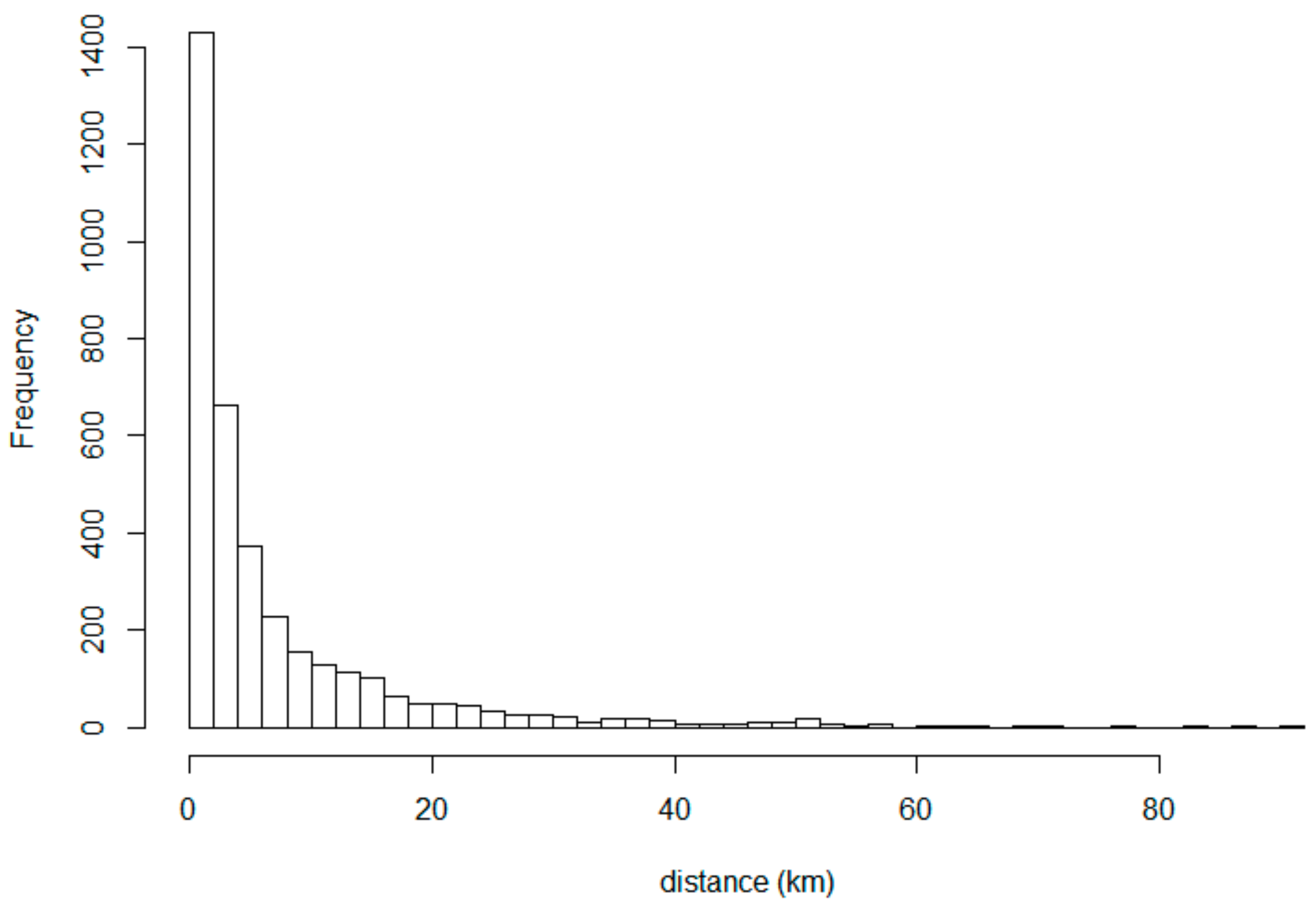
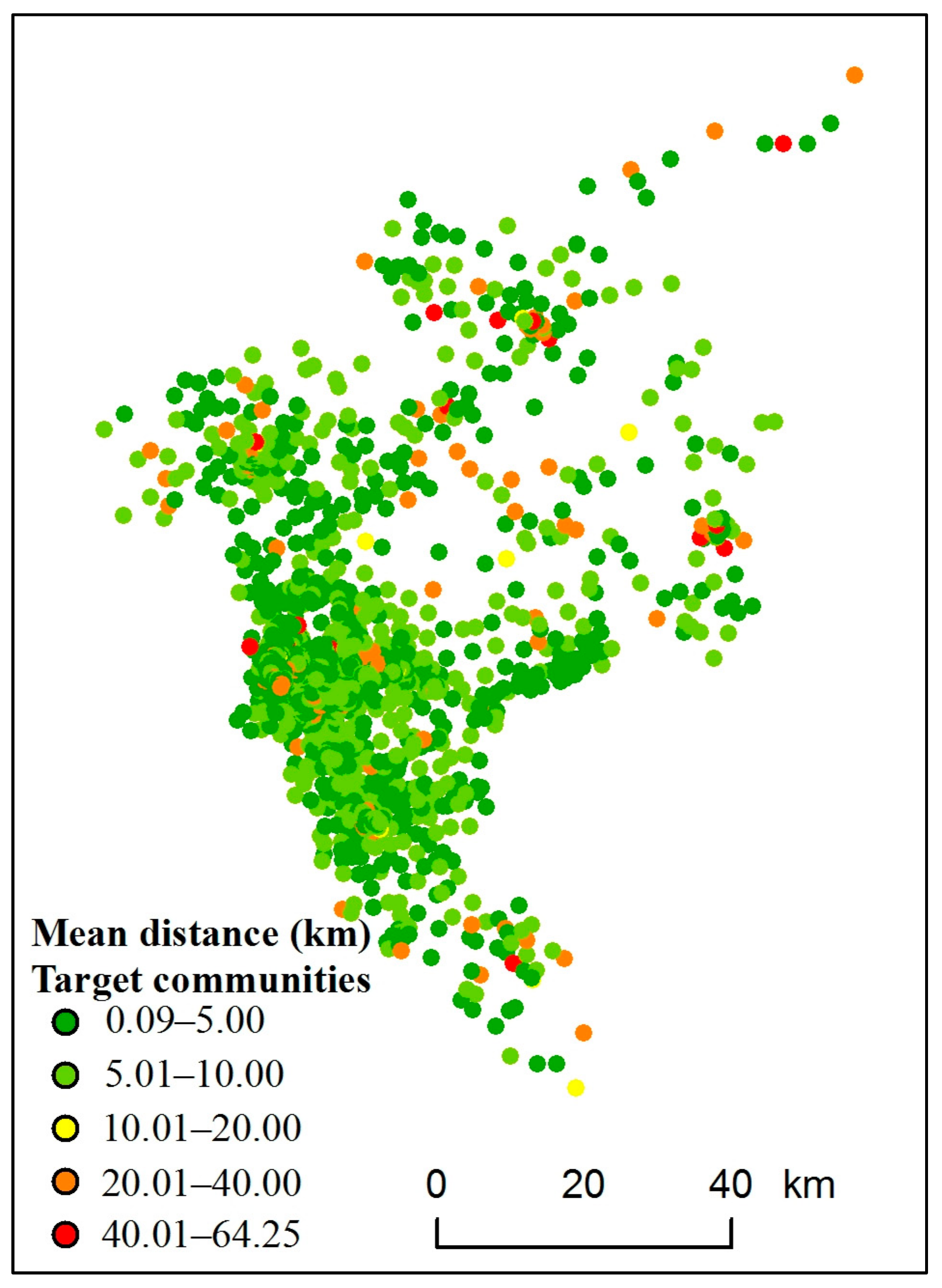
3.1.1. Dependent Variable: Journey-to-Crime Distance

The journey-to-crime distance is defined as the distance between the centroids of the home community and target community as the origin and destination points of a burglary trip, respectively [7]. Since prior research shows that Euclidian distances and distances over the street network are very strongly correlated [13,46], we decided to use Euclidean distances. The reason that we use the centroids of communities instead of their specific coordinates is because most of the addresses could be geocoded correctly at the community level, but not at the house level due to some ambiguous descriptions.
2949 burglaries (78.4 percent) were trips with origins and destinations located in different communities, while the remaining 814 burglaries (21.6 percent) were committed in the home community of the burglar. In order to approximate the journey-to-crime distances for the latter trips, we simulated 100 random points inside each community and calculated the average distance between all pairs of two random points for each community.
The journey-to-crime distance distribution is shown in Figure 1. It shows that the distribution is highly skewed to the left. Following Ackerman and Rossmo [13], we log-transformed the distance for our analyses so that the few cases in the long tail would not be influential outliers and affect the model results too much.
Figure 2 and Figure 3 show the average journey-to-crime distance based on home communities and target communities, respectively. Each point represents the centroid of each community. On the whole, they have similar spatial patterns, that is, most of the short distances are located in the city center and longer distances are located in the north part, east part and south part of the city. However, criminal trips that are longer than 10 km based on the home community have a more dispersed distribution pattern compared to those based at the target community.

3.1.2. Independent Variables
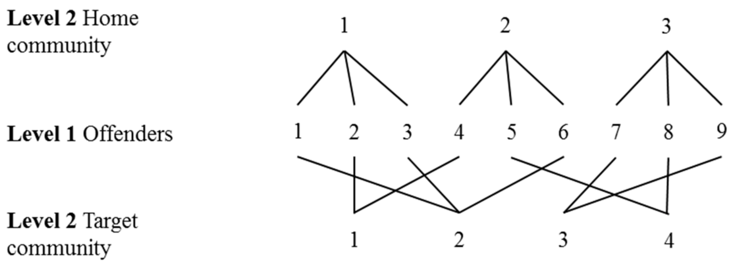
The independent variables are categorized into three groups, including individual-level offender characteristics, offenders’ home community-level characteristics, and target community-level characteristics.
Individual-level characteristics:
Age was measured by subtracting offender’s date of birth from the crime date.
Gender was measured with a dichotomous variable, which scores 1 for male and 0 for female offenders.
In order to measure whether a residential burglar was a local resident, we used information of Hukou for each offender. If the Hukou was ZG City, this variable was coded 1, otherwise it was coded 0.
For each offense, we coded whether it was committed by a solo offender or a group of offenders. This resulted in the co-offending variable, which scores 1 when the residential burglar had at least one co-offender, and 0 means the residential burglar had committed the burglary alone.
Community-level characteristics:
For all residential burglaries analyzed in this study, the home communities of the offenders and the target communities where they committed their burglaries were all among the 2643 communities in ZG City. For this reason, both the independent variables that reflect the characteristics of home communities and those for target communities are described here together.
The number of households was measured to capture the opportunities for burglary, which partly captures the expected benefit for offenders [7,29]. The number of households for each community was obtained from the census data.
We include the average rent price of communities, because this should also be related to the expected benefits of residential burglaries. We calculated these using the midpoints for all the eight rent categories from the census, multiplying those with the exact number of households in each respective rent category (for the lowest category “lower than 100 yuan” and highest category “higher than 3000 yuan”, we used 50 yuan and 4000 yuan, respectively). The average rent for each community was then calculated by dividing the total rent by the number of households. Some communities in rural areas far removed from urban centers have no rental houses. Their average thus is defined as 0. These communities are much poorer than urban communities and rural communities closer to urban regions.
We further include the percentage of houses over 9 floors, because buildings that exceed 9 floors in China are oftentimes equipped with elevators and security guards [47,48]. Offenders might thus escape more easily from buildings lower than 9 floors. We calculated this measure by dividing the number of houses over 9 floors by the total number of households, and multiplied this by 100.
The percentage of local residents captures the degree to which the population in a community is originally from ZG City [32]. We assume that the higher the percentage of local residents in a community, the stronger the informal social control, and therefore the higher the risk for offenders [49]. We used the Hukou information from the census data to distinguish local ZG City residents from the nonlocal residents who came to the city from other parts of China. We calculated the percentage of local residents by dividing the number of local residents by the total number of individuals, and multiplying it by 100.
Road network density was measured by calculating the total length of roads in each community divided by the area size of the community. A higher network density should be related to a lower transportation time, which would imply a lower travel cost [7].
Table 1 displays the descriptive statistics for all variables used in this study. Journey-to-crime distances were on average 7.1 km, which is remarkably similar to the 8.2 km reported in the study on burglary trips in Flanders, Belgium [7]. The burglars were on average just over 27 years old, but the youngest was 9 and the oldest 60. Almost all burglars were male (95.4 percent). 14.7 percent of the burglars were local residents, and 24.6 percent of the burglars had committed the burglary with other offenders.
The same independent variables at the community level were used for both the home communities of the offenders and their burglary target communities. The number of households and road network density had somewhat higher average values for the home communities than for the target communities. For the other variables, including percentage of houses over 9 floors, average rent and percentage of local residents, the home communities had much smaller values than those of target communities.

3.2. Methods

Since the aim of this paper is to disentangle how journey-to-crime distances are affected by both the offenders’ individual-level as well as origin and destination community-level characteristics, it is necessary to apply a multilevel model. Such a model allows us to account for the fact that burglary trips made by offenders from the same community will be more alike than trips by offenders of different communities. We assume that different trips to a particular community will also be more alike than trips to different target communities. As such, the trips are nested in both origin and destination communities. A multilevel model allows us not only to explore the relationship between the dependent variable and the independent variables, but also shows much journey-to-crime trips vary at each level [50]. Standard multilevel models require that the observations must have a strictly nested structure. However, our observations are not perfectly hierarchically nested. For each journey-to-crime trip, the origin corresponds to the home community of the offender, whereas the destination is the target community; and because offenders from the same community could have committed burglaries in different communities while a particular community could also have been targeted by offenders from different communities, our data have a so-called cross-classified structure (see Figure 4). We thus distinguish three different levels, the individual offender level and two community levels. Cross-classified multilevel models, which have already been widely used in other domains [51,52], have not yet been used in journey-to-crime studies, but they are well-suited to analyze data of this structure [53]. In total, we had 3763 crime trips nested in 1117 home communities and 1382 target communities.
We estimate three different random intercept models. These models allow us to show how the intercept (the mean journey-to-crime distance) varies over the different levels. The first model was a null model without any independent variables, which decomposes the intercept variance into the three different levels. In the second model, we included both the individual-level and target community-level variables. The third model is the full model, in which variables at all three levels were included. The formulae for the three different models are presented below.
Null   model   0 :   Y i ( j , k ) = β 0 + R i j k + T 0 j + H 0 k ,
model   1 :   Y i ( j , k ) = β 0 + a = 1 A β a x a i + b = 1 B β b x b j + R i j k + T 0 j + H 0 k   ,
full   model   2 :   Y i ( j , k ) = β 0 + a = 1 A β a x a i + b = 1 B β b x b j + c = 1 C β c x c k + R i j k + T 0 j + H 0 k   ,
where Y i ( j , k ) is the journey-to-crime distance for residential burglar i between his/her home community j and target community k. β 0 is the grand mean intercept of the model. The following three items, a = 1 A β a x a i , b = 1 B β b x b j and c = 1 C β c x c k , are coefficients ( β a ,   β b ,   β c ) and variables ( x a i ,   x b j ,   x c k ) for individual-level, target community-level and home community-level characteristics, respectively. These are the fixed parts of the model. The following three items, R i j k , T 0 j and H 0 k , are the random parts of the model. The intercept variance is decomposed into the following three different levels:
V a r ( R i j k ) = σ 2   ( individual level   variance ) ,
V a r ( T 0 j ) = τ T 2   ( target   community level   variance ) ,
V a r ( H 0 k ) = τ H 2   ( home   community level   variance ) .
With the decomposed variances, the intra-class correlation coefficient (ICC) can be calculated, which provides a measure for the proportion of the intercept variance at each level. When the ICC is close to zero, the difference between groups is small and a traditional regression model would have been appropriate. A relatively large value of ICC indicates that a multilevel model is more appropriate for the data. The formulae of ICC are as follows.
I C C T = τ T 2 τ T 2 + τ H 2 + σ 2   ( intra target   community ) ,
I C C H = τ H 2 τ T 2 + τ H 2 + σ 2   ( intra home   community ) ,
where I C C T is the correlation between journey-to-crime distances of residential burglars who lived in the same target communities and committed crimes in different home communities. I C C H is the correlation between journey-to-crime distances of residential burglars who lived in the same home communities and committed crimes in different target communities.
All of the data analysis and model estimation were done in Stata 15/MP and R 3.4.3. Maps were plotted in ArcGIS 10.3. Stata was used for data preprocessing, and the restricted maximum likelihood (REML) estimation method [54] from the lme4 package [55] in R was used for the estimation of the cross-classified multilevel model. All the independent variables were grand mean centered before entering them in the models [50]. Thus, the intercept of each model represents the mean log distance.

4. Results

Table 2 shows a total intercept variance of 1.824 in the null model, which is the sum of 0.276 for the target community level, 0.539 for the home community level, and 1.009 for the individual level. Thus, 29.6 percent of the total variance is associated with the home communities of the offenders ( I C C H ), while 15.1 percent is associated with the burglary target communities ( I C C T ). This shows that it is important to decompose the variance in journey-to-crime distances into different levels, and that the cross-classified multilevel model fits this type of analysis well.
Model 1 contains individual-level offender characteristics and target community-level characteristics. After including these variables, the total intercept variance decreases to 1.767, which further decreases in the full model when also the origin community-level variables are included (1.719). So, with the variables included in the full model, we are able to explain 6 percent ((1.824 − 1.719)/1.824) of the total variance of journey-to-crime distances.
Model 1 shows that both the age of the offender as well as co-offending are related to longer journey-to-crime distances. Only the variables of percentage of local residents and road network density in the target area level have significant effects on offenders’ travel distance. Higher percentages of local residents would result in longer journey-to-crime distances, while denser road networks would discourage offenders’ mobility.
As for model 2, one year of age corresponds with a 0.7 percent increase in the distance of the burglary trip. Burglary trips of co-offenders are much longer (b = 0.319) than those of burglars who commit the burglary alone.
With respect to the characteristics of the target community level, the full model shows that the percentage of local residents in the community is statistically significantly related to longer journey-to-crime distances. A one-percent increase corresponds with an increase of 0.8 percent in the distance of the burglary trip. So, communities with more local residents attract burglars from over longer distances. The road network density shows a statistically significant negative impact on the length of the burglary trip. An increase of 1 km/km2 of the road network density corresponds with a decrease of 1 percent in the distance of the crime trip.
For the home community level, we observe that a higher average rent significantly reduces the distances residential burglars travel to commit a burglary. The percentage of local residents also shows a statistically significant negative impact on journey-to-crime distances. With a 1 percent increase of local residents in the home community of a burglar, the distance he travels to commit a burglary decreases with 0.5 percent. The road network density of the home community also significantly impacts the journey-to-crime distances (b = −0.018). Burglars from communities with a higher road network density commit their burglaries closer-by.

5. Conclusions and Discussion

This study used a cross-classified multilevel model to examine residential burglars’ origin and destination effects on their journey-to-crime distances. This way of modeling provides a more comprehensive framework to analyze the benefits, risks and costs offenders may face when making their crime trips. This novel approach to the study of journey-to-crime distances avoids incorrect estimation of the effects at different levels. The results show that the home area, the target area as well as the individual level are all significantly related to the journey-to-crime distance.
The home communities of burglars account for about a third of the variance in journey-to-crime distances. Maybe offenders first search targets in or nearby their own residential community before traveling further, because the travel cost is then minimal and they are most familiar with the benefits and risks involved. Average rent, road network density and percentage of local residents in the home area each were shown to reduce the residential burglars’ mobility. If residential burglars live in more affluent communities, their willingness to travel further in search of a burglary target would be decreased. We believe that is because those living in high rent areas would already be able to obtain sufficient reward without going too far. Well-developed road networks probably improve the accessibility of targets inside the residential areas of offenders, which also reduces the need to travel over longer distances. Home areas with more local residents seem to cause the offenders to travel over shorter distances. Although we assumed that having a higher percentage of local residents in a community often implies higher informal social control, more local residents also means more affluent targets, and the increasing anonymity of modern society has weakened the social network and therefore the informal social control [56]. However, neither the number of households inside the home community nor the percentage of high-rise buildings have an effect on journey-to-crime distances. From these results, we infer that accessible and profitable targets near home will discourage offenders to travel over long distances, whereas the absence of profitable targets in the home community may incentivize offenders to travel to communities further away.
Compared to the home community, target communities account for a smaller part of the variance in journey-to-crime distances. Nevertheless, target communities with more local residents attract offenders from over longer distances. The reason may be that more local residents probably provide wealthier targets. However, if these communities also have higher levels of informal social control and thus a higher risk to offenders, this apparently does not outweigh the effects of the higher potential rewards. Offenders travel less far if target communities have a high road network density, which is not in line with the expectation that a higher road network density would reduce the travel costs and thus be related to a longer crime trip distance [7]. It could be that an increase in road network density is related to more ambient population, which would increase the risk of detection. Frith, Johnson [39] also argue that street networks are related to both levels of guardianship and accessibility and opportunities. In this research, it seems that road network density in residential burglars’ home areas is more related to opportunities, whereas in target areas it seems more related to levels of guardianship.
The individual characteristics of residential burglars are most important for understanding the variation in journey-to-crime distances, as they account for more than 55 percent of the total variance. We observed no differences between male and female burglars nor between local and nonlocal burglars. However, older burglars have longer crime trips, a finding consistent with that of Nichols [57]. Older burglars are probably more experienced in crime location selection and have a larger awareness space, whereas the young burglars often limit themselves to around their living communities [17,58]. Burglars who commit the burglaries with co-offenders travel further, which is in line with the idea that co-offenders have a larger combined awareness space, leading them to travel longer distances [15,17].
In general, many of our conclusions are in accordance with the literature, but we improve upon previous studies by further decomposing the variance in journey-to-crime distances. We showed how much journey-to-crime distances for residential burglaries in ZG City are affected by both individual and origin and destination community differences. Most findings fit with rational choice theory and crime pattern theory, which suggest that offenders in China indeed prefer benefit maximization, and risk and cost minimization in their awareness spaces, though care is required regarding the operationalization of the concepts in the Chinese context. However, this study also provides new insights. Firstly, home communities account for a larger part of the variance in burglars’ journey-to-crime distances than target communities. Secondly, target communities with fewer nonlocal residents who migrated to ZG City from other parts in China draw burglars from longer distances. Previous studies showed that areas with a higher proportion of local residents may attract fewer offenders because of their higher levels of informal social control [56]. However, we show that these areas attract burglars from over longer distances.
It should be pointed out that this study did not consider effects of household registration places of nonlocal offenders on their distances of journey to crime. Because nonlocals who originally came from the same cities or provinces often cluster together in tightknit social networks, residential burglars from the same migrant groups might show similar offending patterns. Additionally, although it is inevitable, the deletion of cases without key information, like home and target addresses, might have potential effects on model results. With the improvement in the accuracy of the crime records, this problem can be properly dealt with in the future. Nevertheless, the novel modeling approach and new findings and insights presented in this study make it a meaningful contribution to the journey-to-crime literature.

Author Contributions

Conceptualization, L.X., L.L. and S.Z.; Formal analysis, L.X.; Funding acquisition, L.L. and S.Z.; Methodology, L.X. and S.R.; Supervision, L.L. and S.Z.; Writing—original draft, L.X. and G.S.; Writing—review & editing, L.L., G.S. and S.R.

Funding

This research was funded by the National Key R&D Program of China (Nos. 2018YFB0505500, 2018YFB0505503), Key Program of National Natural Science Foundation of China (No. 41531178), Key Project of Science and Technology Program of Guangzhou City, China (No. 201804020016), Research Team Program of Natural Science Foundation of Guangdong Province, China (No. 2014A030312010) and National Science Fund for Excellent Young Scholars (No. 41522104).

Acknowledgments

The authors would like to thank the editor and the three anonymous reviewers for their helpful feedback.

Conflicts of Interest

The authors declare no conflict of interest.

References

  1. Rossmo, K. Geographic Profiling; CRC Press: Boca Raton, FL, USA, 2000. [Google Scholar]
  2. Brantingham, P.L.; Brantingham, P.J. Nodes, paths and edges: Considerations on the complexity of crime and the physical environment. J. Environ. Psychol. 1993, 13, 3–28. [Google Scholar] [CrossRef]
  3. Brantingham, P.L.; Brantingham, P.J. Notes on the Geometry of Crime. In Environmental Criminology; Brantingham, P.J., Brantingham, P.L., Eds.; Sage Publications: Beverly Hills, CA, USA, 1981; pp. 27–54. [Google Scholar]
  4. Cornish, D.B.; Clarke, R.V. The Reasoning Criminal: Rational Choice Perspective on Offending; Springer: Berlin, Germany, 1986. [Google Scholar]
  5. Wheeler, A. The Moving Home Effect: A Quasi Experiment Assessing Effect of Home Location on the Offence Location. J. Quant. Criminol. 2012, 28, 587–606. [Google Scholar] [CrossRef]
  6. Block, R.; Galary, A.; Brice, D. The Journey to Crime: Victims and Offenders Converge in Violent Index Offences in Chicago. Secur. J. 2007, 20, 123–137. [Google Scholar] [CrossRef]
  7. Vandeviver, C.; van Daele, S.; Beken, T.V. What makes long crime trips worth undertaking? Balancing costs and benefits in burglars’ journey to crime. Br. J. Criminol. 2015, 55, 399–420. [Google Scholar] [CrossRef]
  8. Capone, L.D.; Nichols, W.W. Urban Structure and Criminal Mobility. Am. Behav. Sci. 1976, 20, 199–213. [Google Scholar] [CrossRef]
  9. Rattner, A.; Portnov, B.A. Distance decay function in criminal behavior: A case of Israel. Ann. Reg. Sci. 2007, 41, 673–688. [Google Scholar] [CrossRef]
  10. Van Koppen, P.J.; Keijser, J.W. Desisting Distance Decay: On the Aggregation of Individual Crime Trips. Criminology 1997, 35, 505–515. [Google Scholar] [CrossRef]
  11. Rengert, F.G.; Piquero, A.R.; Jones, P.R. Distance Decay Reexamined. Criminology 1999, 37, 427–446. [Google Scholar] [CrossRef]
  12. Townsley, M.; Sidebottom, A. All offenders are equal, but some are more equal than others: Variation in journeys to crime between offenders. Criminology 2010, 48, 897–917. [Google Scholar] [CrossRef]
  13. Ackerman, M.J.; Rossmo, D.K. How far to travel? A multilevel analysis of the residence-to-crime distance. J. Quant. Criminol. 2015, 31, 237–262. [Google Scholar] [CrossRef]
  14. Andresen, A.M.; Frank, R.; Felson, M. Age and the distance to crime. Criminol. Crim. Justice 2014, 14, 314–333. [Google Scholar] [CrossRef]
  15. Levine, N.; Lee, P. Journey-to-Crime by Gender and Age Group in Manchester, England, in Crime Modeling and Mapping Using Geospatial Technologies; Leitner, M., Ed.; Springer: Dordrecht, The Netherlands, 2013; pp. 145–178. [Google Scholar]
  16. Johnson, T.L.; Taylor, R.B.; Ratcliffe, J.H. Need drugs, will travel? The distances to crime of illegal drug buyers. J. Crim. Justice 2013, 41, 178–187. [Google Scholar] [CrossRef]
  17. Van Daele, S.; Beken, T.V. Outbound offending: The journey to crime and crime sprees. J. Environ. Psychol. 2011, 31, 70–78. [Google Scholar] [CrossRef] [Green Version]
  18. Bernasco, W.; Nieuwbeerta, P. How do residential burglars select target areas? A new approach to the analysis of criminal location choice. Br. J. Criminol. 2005, 45, 296–315. [Google Scholar] [CrossRef]
  19. Ruiter, S. Crime Location Choice: State-of-the-Art and Avenues for Future Research. In The Oxford Handbook of Offender Decision Making; Bernasco, W., Elffers, H., Gelder, J.-L.V., Eds.; Oxford University Press: Oxford, UK, 2017; pp. 398–420. [Google Scholar]
  20. Morselli, C.; Royer, M.-N. Criminal Mobility and Criminal Achievement. J. Res. Crime Délinq. 2008, 45, 4–21. [Google Scholar] [CrossRef]
  21. Chamberlain, W.A.; Boggess, L.N. Relative Difference and Burglary Location: Can Ecological Characteristics of a Burglar’s Home Neighborhood Predict Offense Location? J. Res. Crime Délinq. 2016, 53, 872–906. [Google Scholar] [CrossRef]
  22. Rengert, G.F. Burglary in Philadelphia: A Critique of an Opportunity Structure Model. In Environmental Criminology; Brantingham, P.J., Brantingham, P.L., Eds.; Sage Publications: Beverly Hills, CA, USA, 1981; pp. 189–202. [Google Scholar]
  23. Smith, T.S. Inverse Distance Variations for the Flow of Crime in Urban Areas. Soc. Forces 1976, 54, 802–815. [Google Scholar] [CrossRef]
  24. Reynald, D.; Averdijk, M.; Elffers, H.; Bernasco, W. Do Social Barriers Affect Urban Crime Trips? The Effects of Ethnic and Economic Neighbourhood Compositions on the Flow of Crime in The Hague, The Netherlands. Built Environ. 2008, 34, 21–31. [Google Scholar] [CrossRef]
  25. Bennett, T.; Wright, R. Burglars on Burglary: Prevention and the Offender; Gower Publishing Company: Brookfield, VT, USA, 1984. [Google Scholar]
  26. Nagin, S.D.; Paternoster, R. Personal Capital and Social Control: The Deterrence Implications of a Theory of Individual Differences in Criminal Offending. Criminology 1994, 32, 581–606. [Google Scholar] [CrossRef]
  27. Rengert, G.F. The Journey to Crime, in Punishment, Places and Perpetrators; Bruinsma, G., Elffers, H., de Keijser, J., Eds.; Willan: Devon, UK, 2004; pp. 169–181. [Google Scholar]
  28. Vandeviver, C.; Neutens, T.; Van Daele, S.; Geurts, D.; Vander Beken, T. A discrete spatial choice model of burglary target selection at the house-level. Appl. Geogr. 2015, 64, 24–34. [Google Scholar] [CrossRef] [Green Version]
  29. Townsley, M.; Birks, D.; Bernasco, W.; Ruiter, S.; Johnson, S.D.; White, G.; Baum, S. Burglar Target Selection: A Cross-national Comparison. J. Res. Crime Délinq. 2015, 52, 3–31. [Google Scholar] [CrossRef] [PubMed]
  30. Loughran, T.A.; Paternoster, R.; Piquero, A.R.; Pogarsky, G. On Ambiguity in Perceptions of Risk: Implications for Criminal Decision Making and Deterrence. Criminology 2011, 49, 1029–1061. [Google Scholar] [CrossRef]
  31. Lim, H.; Wilcox, P. Crime-Reduction Effects of Open-street CCTV: Conditionality Considerations. Justice Q. 2017, 34, 597–626. [Google Scholar] [CrossRef]
  32. Zhang, L.; Messner, S.F.; Liu, J. A Multilevel Analysis of the Risk of Household Burglary in the City of Tianjin, China. Br. J. Criminol. 2007, 47, 918–937. [Google Scholar] [CrossRef]
  33. Jiang, S.; Lambert, E.; Wang, J. Correlates of formal and informal social/crime control in China: An exploratory study. J. Crim. Justice 2007, 35, 261–271. [Google Scholar] [CrossRef]
  34. Jiang, S.; Land, K.C.; Wang, J. Social Ties, Collective Efficacy and Perceived Neighborhood Property Crime in Guangzhou, China. Asian J. Criminol. 2013, 8, 207–223. [Google Scholar] [CrossRef]
  35. Braga, A.A.; Clarke, R.V. Explaining High-Risk Concentrations of Crime in the City: Social Disorganization, Crime Opportunities, and Important Next Steps. J. Res. Crime Délinq. 2014, 51, 480–498. [Google Scholar] [CrossRef]
  36. Addington, A.L.; Rennison, C.M. Keeping the Barbarians Outside the Gate? Comparing Burglary Victimization in Gated and Non-Gated Communities. Justice Q. 2015, 32, 168–192. [Google Scholar] [CrossRef]
  37. Summers, L.; Johnson, S.D. Does the Configuration of the Street Network Influence Where Outdoor Serious Violence Takes Place? Using Space Syntax to Test Crime Pattern Theory. J. Quant. Criminol. 2017, 33, 397–420. [Google Scholar] [CrossRef]
  38. Davies, T.; Johnson, S.D. Examining the Relationship Between Road Structure and Burglary Risk Via Quantitative Network Analysis. J. Quant. Criminol. 2015, 31, 481–507. [Google Scholar] [CrossRef]
  39. Frith, J.M.; Johnson, S.D.; Fry, H.M. Role of the street network in burglars’ spatial decision-making. Criminology 2017, 55, 344–376. [Google Scholar] [CrossRef]
  40. Zhou, S.; Deng, L.; Kwan, M.P.; Yan, R. Social and spatial differentiation of high and low income groups out-of-home activities in Guangzhou, China. Cities 2015, 45, 81–90. [Google Scholar] [CrossRef]
  41. Rengert, G.F. Some effects of being female on criminal spatial behavior. Pa. Geogr. 1975, 13, 10–18. [Google Scholar]
  42. Pettiway, L.E. Copping crack: The travel behavior of crack users. Justice Q. 1995, 12, 499–524. [Google Scholar] [CrossRef]
  43. Brent, S. Individual differences in distance travelled by serial burglars. J. Investig. Psychol. Offender Profiling 2004, 1, 53–66. [Google Scholar]
  44. Chen, J.; Liu, L.; Zhou, S.; Xiao, L.; Jiang, C. Spatial Variation Relationship between Floating Population and Residential Burglary: A Case Study from ZG, China. ISPRS Int. J. Geo-Inf. 2017, 6, 246. [Google Scholar] [CrossRef]
  45. Liu, L.; Feng, J.; Ren, F.; Xiao, L. Examining the relationship between neighborhood environment and residential locations of juvenile and adult migrant burglars in China. Cities 2018. [Google Scholar] [CrossRef]
  46. Groff, E.; McEwen, J.T. Disaggregating the Journey to Homicide, in Geographic Information Systems and Crime Analysis; Wang, F., Ed.; Idea Group: Hershey, PA, USA, 2005; pp. 60–83. [Google Scholar]
  47. Yang, G.; Liu, L.; He, S.; Xu, C. Environmental impacts on burglary victimization in gated communities: A multi-level analysis in Guangzhou. Trop. Geogr. 2016, 36, 610–618. [Google Scholar]
  48. Xiao, L.; Liu, L.; Song, G.; Zhou, S.; Long, D.; Feng, J. Impacts of community environment on residential burglary based on rational choice theory. Geogr. Res. 2016, 36, 2479–2491. [Google Scholar]
  49. Jiang, S.; Wang, J.; Lambert, E. Correlates of informal social control in Guangzhou, China neighborhoods. J. Crim. Justice 2010, 38, 460–469. [Google Scholar] [CrossRef]
  50. Snijders, T.A.B.; Bosker, R.J. Multilevel Analysis: An Introduction to Basic and Advanced Multilevel Modeling, 2nd ed.; Sage: Los Angeles, CA, USA, 2012. [Google Scholar]
  51. Park, H.-C.; Kim, D.K.; Kho, S.Y.; Park, P.Y. Cross-classified multilevel models for severity of commercial motor vehicle crashes considering heterogeneity among companies and regions. Accid. Anal. Prev. 2017, 106, 305–314. [Google Scholar] [CrossRef] [PubMed]
  52. Townsend, N.; Rutter, H.; Foster, C. Age differences in the association of childhood obesity with area-level and school-level deprivation: Cross-classified multilevel analysis of cross-sectional data. Int. J. Obes. 2012, 36, 45. [Google Scholar] [CrossRef] [PubMed]
  53. Rasbash, J.; Goldstein, H. Efficient analysis of mixed hierarchical and cross-classified random structures using a multilevel model. J. Educ. Behav. Stat. 1994, 19, 337–350. [Google Scholar] [CrossRef]
  54. Fox, J. Applied Regression Analysis and Generalized Linear Models; Sage Publications: Thousand Oaks, CA, USA, 2015. [Google Scholar]
  55. Bates, D.; Mächler, M.; Bolker, B.; Walker, S. Fitting Linear Mixed-Effects Models Using lme4. J. Stat. Softw. 2015, 67, 1–48. [Google Scholar] [CrossRef]
  56. Song, G.; Liu, L.; Bernasco, W.; Zhou, S.; Xiao, L.; Long, D. Theft from the person in urban China: Assessing the diurnal effects of opportunity and social ecology. Habitat Int. 2018, 78, 13–20. [Google Scholar] [CrossRef]
  57. Nichols, W.W. Mental Maps, Social Characteristics, and Criminal Mobility. In Crime: A Spatial Perspective; Columbia University Press: New York, NY, USA, 1980; pp. 156–166. [Google Scholar]
  58. Van Koppen, P.J.; Jansen, R.W.J. The Road to the Robbery: Travel Patterns in Commercial Robberies. Br. J. Criminol. 1998, 38, 230–246. [Google Scholar] [CrossRef]
Figure 1. Distribution of journey-to-crime distances of residential burglary trips in ZG City, China.
Ijgi 07 00325 g001
Figure 2. Mean distance at the home community level.
Ijgi 07 00325 g002
Figure 3. Mean distance at the target community-level.
Ijgi 07 00325 g003
Figure 4. The cross-classified multilevel data structure.
Ijgi 07 00325 g004
Table 1. Descriptive statistics of dependent and independent variables.
TheoryVariableMeanStd. Dev.Min.Max.
Dependent variable
Distance (km)7.14210.2920.09490.403
Log distance (km)1.1721.289−2.3624.504
Individual-level variables
Crime pattern theoryAge27.6988.6949.00065.000
Gender (male = 1)0.9540.21001
Local resident (yes = 1)0.1470.35401
Co-offending (yes = 1)0.2460.43101
Target community-level variables
Rational choice theorybenefitNumber of households (/1000 households)3.1073.0340.02921.456
benefitAverage rent (1000 yuan per month)0.5250.5190.0004.000
riskPercentage of houses over 9 floors (%)9.34120.7010.000100.000
riskPercentage of local residents (%)56.59125.8092.558100.000
costRoad network density (km/km2)9.1556.5350.19955.902
Home community-level variables
Rational choice theorybenefitNumber of households (/1000 households)3.4223.15198.00021,456.000
benefitAverage rent (1000 yuan per month)0.4540.3920.0004000.000
riskPercentage of houses over 9 floors (%)6.04915.0110.000100.000
riskPercentage of local residents (%)51.44126.2242.558100.000
costRoad network density (km/km2)9.2576.2480.19946.329
Table 2. Cross-classified multilevel models of (logged) journey-to-crime distances.
Null Model 0Model 1Full Model 2
Coefficientt-RatioCoefficientt-RatioCoefficientt-Ratio
(Intercept)1.107 ***31.7001.062 ***29.9861.096 ***30.493
Individual level
Age 0.006 **2.8260.007 **3.057
Gender (male = 1) 0.0100.102−0.015−0.162
Local resident (yes = 1) 0.0721.1120.0801.208
Co-offending (yes = 1) 0.323 ***7.3160.319 ***7.261
Target community level
Number of households (/1000 households) 0.0161.3650.0181.532
Average rent (1000 yuan per month) 0.0190.3050.0730.166
Percentage of houses over 9 floors (%) 0.0010.3790.0010.571
Percentage of local residents (%) 0.008 ***6.5300.008 ***6.846
Road network density (km/km2) −0.016 ***−4.080−0.010 **−2.621
Home community level
Number of households (/1000 households) −0.006−0.408
Average rent (1000 yuan per month) −0.3230 ***−3.849
Percentage of houses over 9 floors (%) 0.0000.019
Percentage of local residents (%) −0.005 **−2.990
Road network density (km/km2) −0.018 **−3.497
Target community-level variance0.276 0.227 0.210
Home community-level variance0.539 0.548 0.517
Individual-level variance1.009 0.991 0.993
Total variance1.824 1.767 1.719
Note: * p < 0.05, ** p < 0.01, *** p < 0.001.

