Automatic Parametrization and Shadow Analysis of Roofs in Urban Areas from ALS Point Clouds with Solar Energy Purposes


Abstract
:1. Introduction
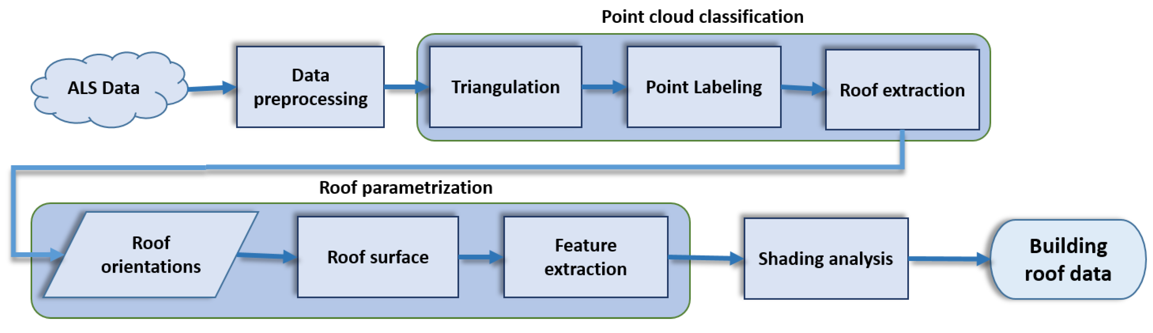
2. Methodology
2.1. Data Preprocessing
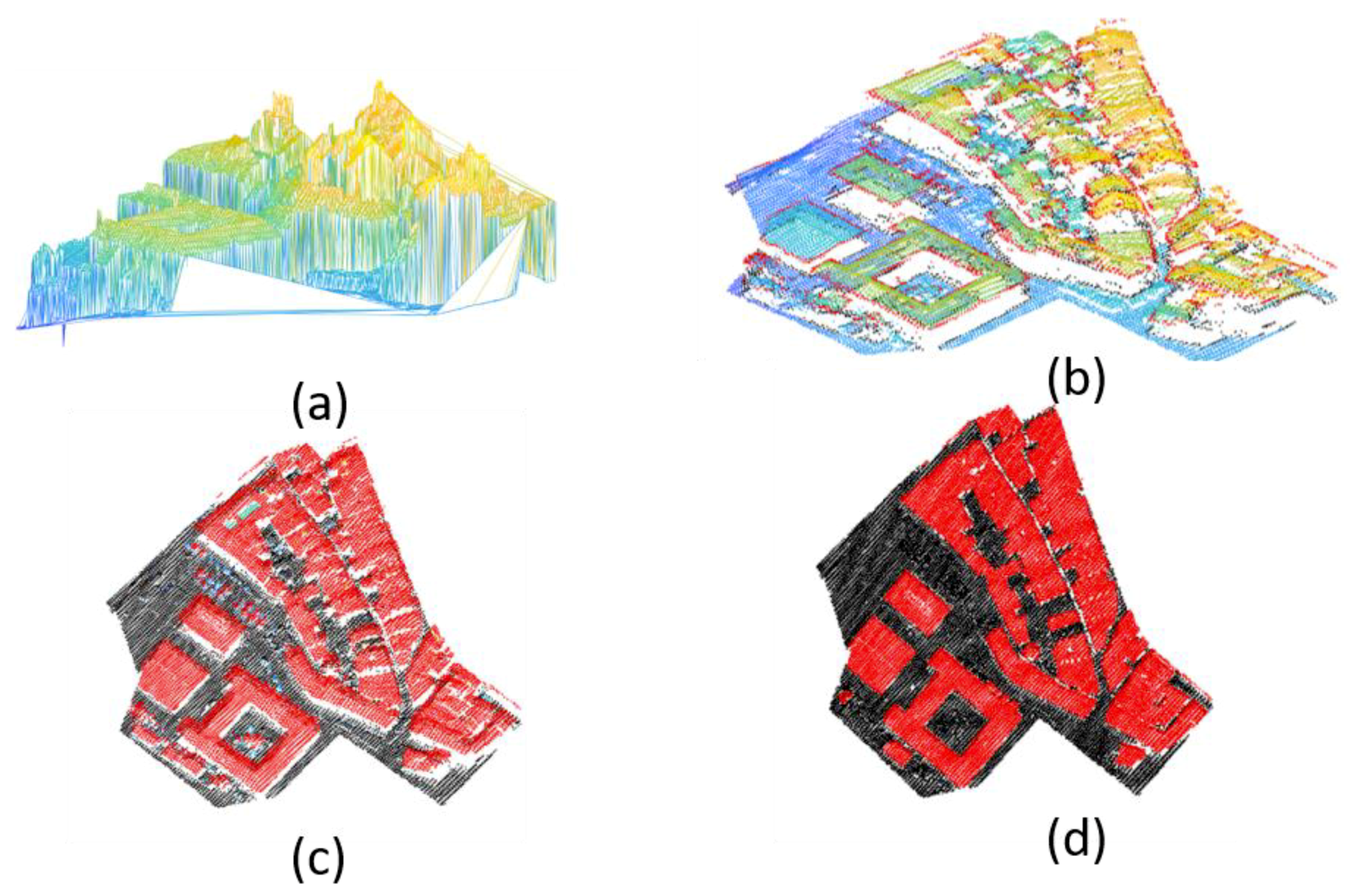
2.2. Point Cloud Classification
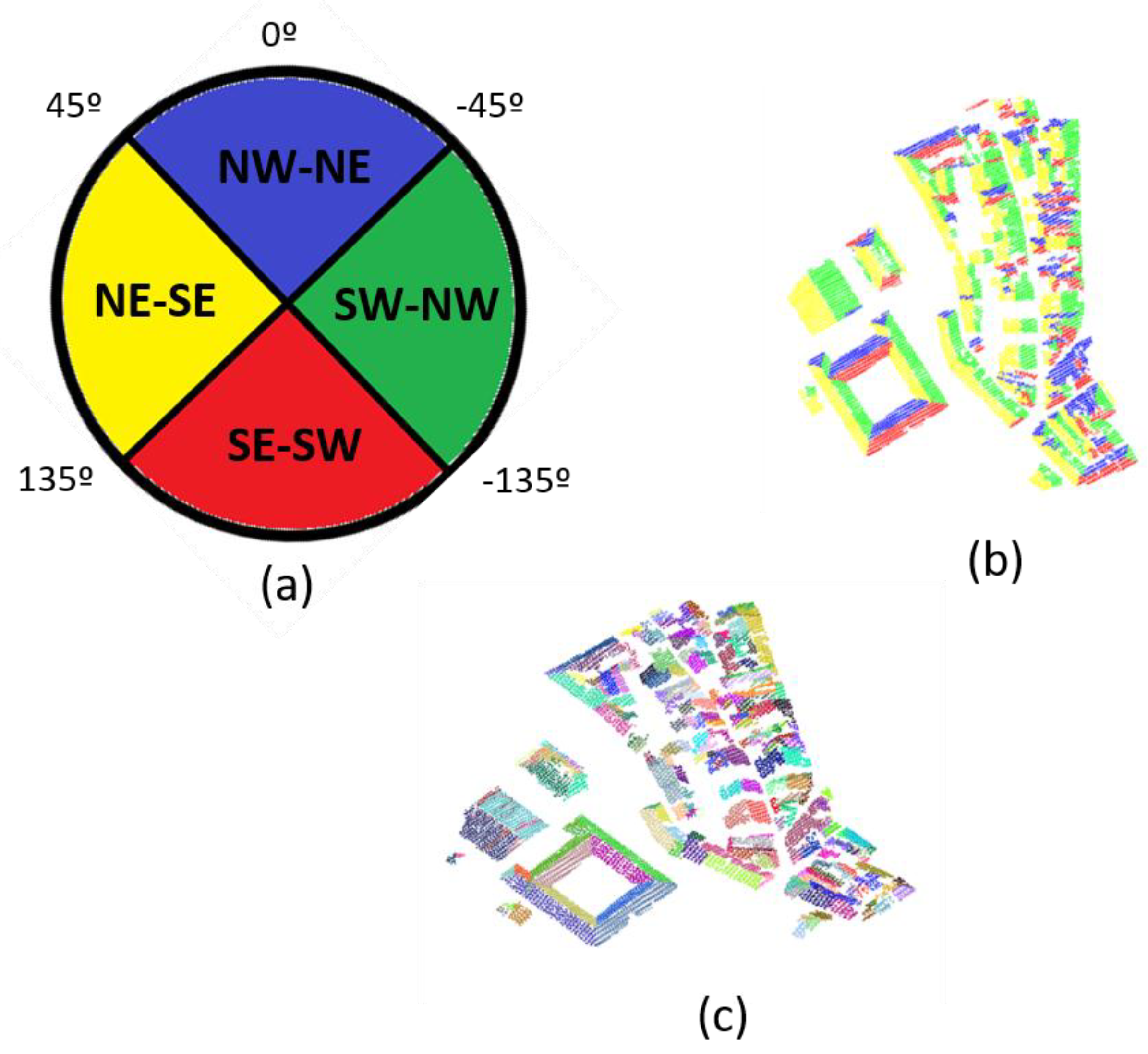
2.3. Roof Parametrization
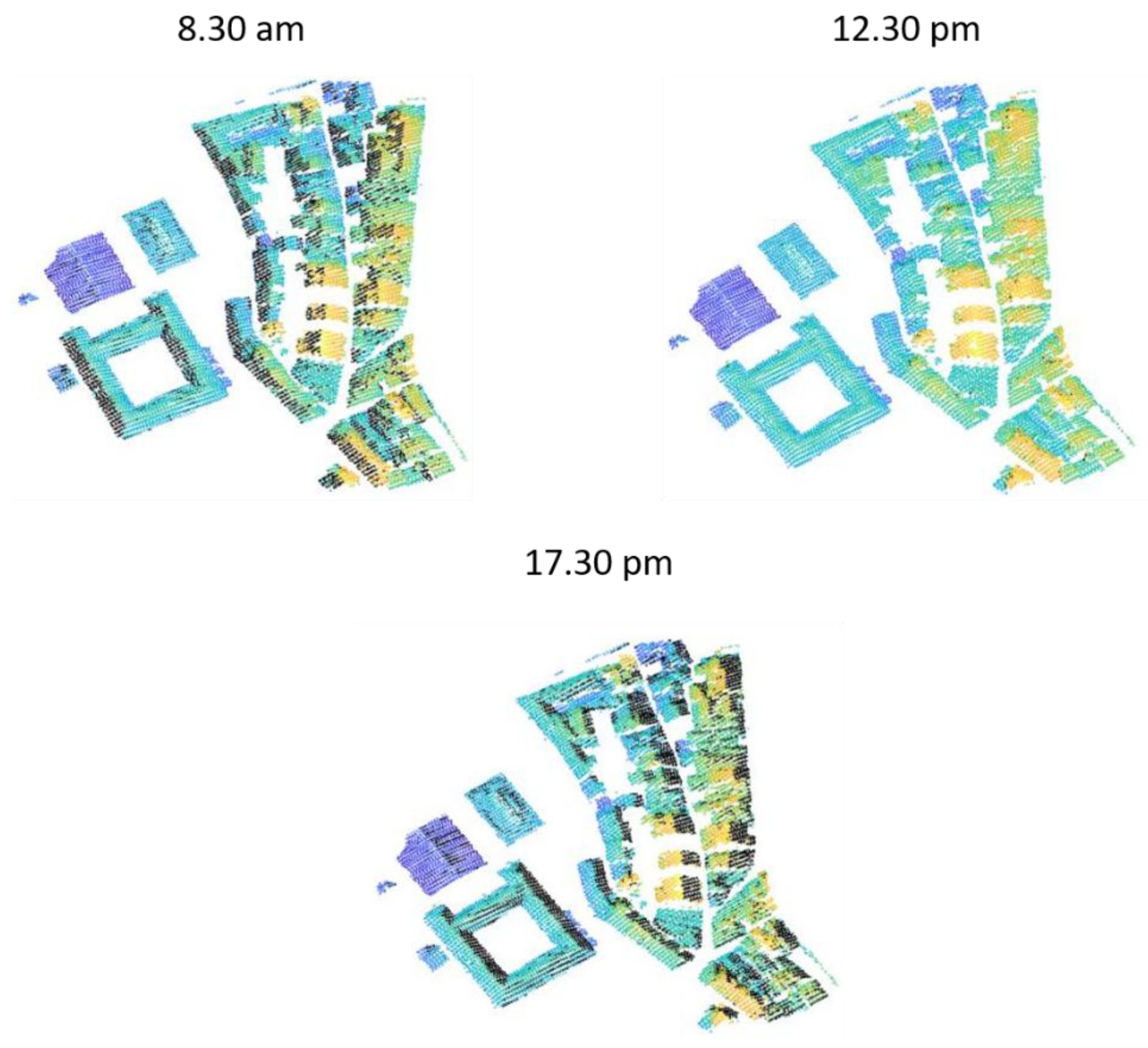
2.4. Shading Analysis
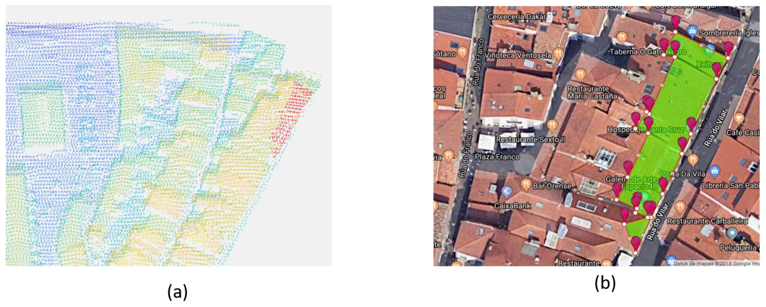
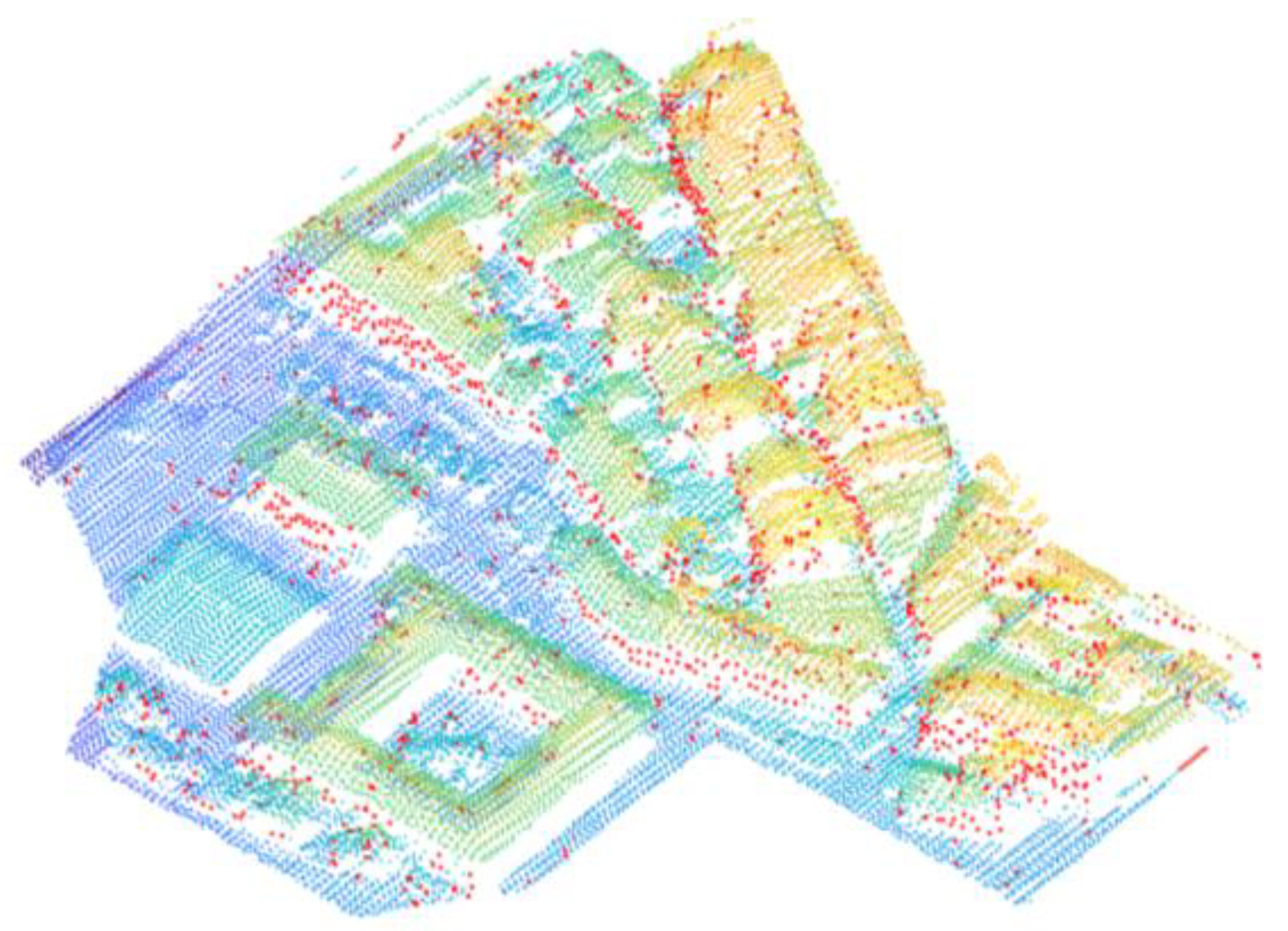
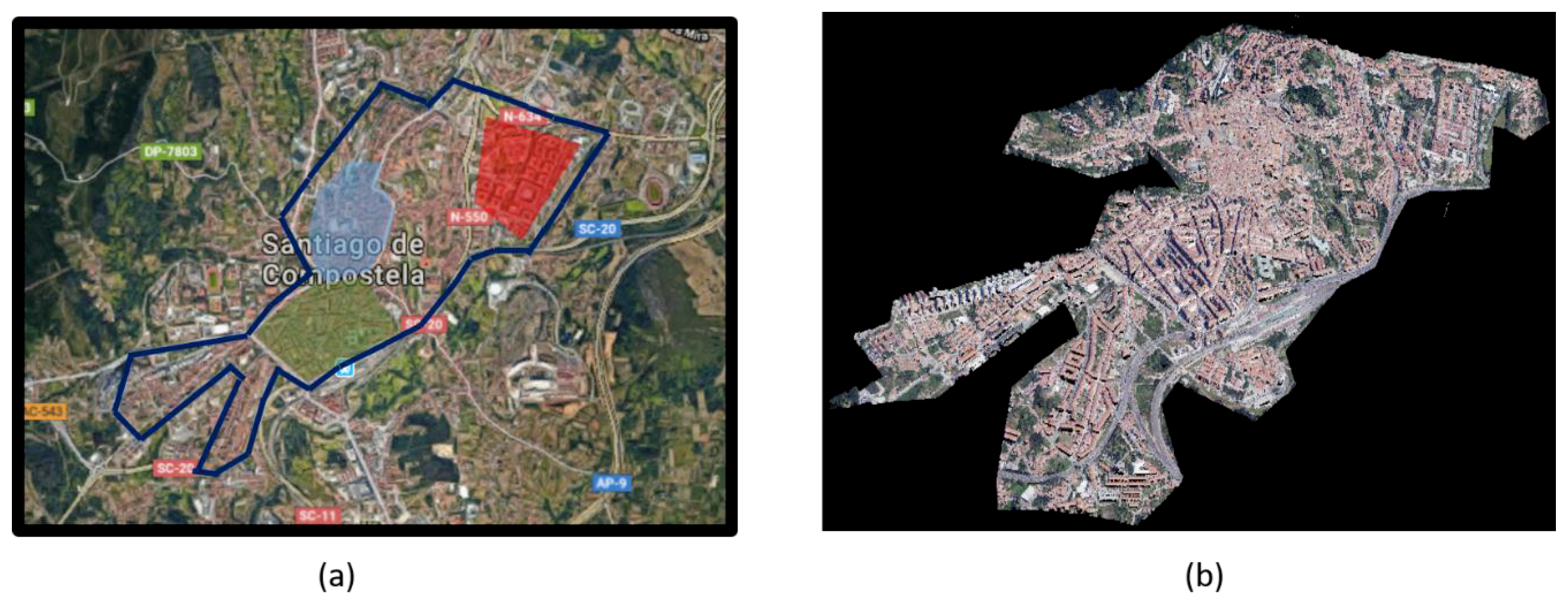
3. Case Study
4. Results and Discussion
4.1. Roof Parametrization
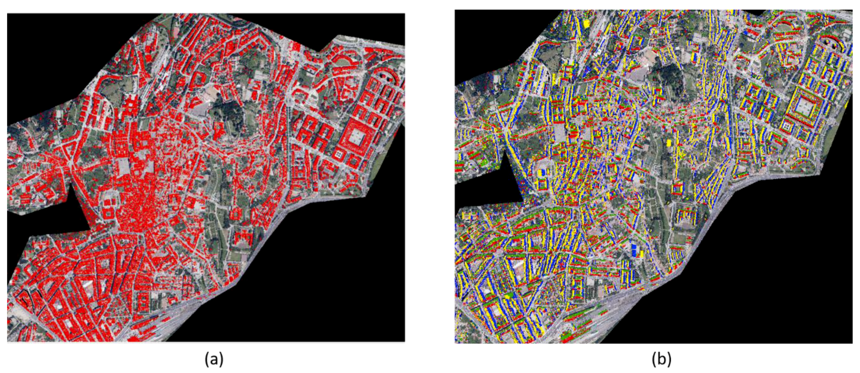
4.2. Roof Classification and Shading Analysis
5. Conclusions
Author Contributions
Funding
Conflicts of Interest
References
- European Commission. Energy Performance of Buildings Directive. Available online: http://resource.npl.co.uk/docs/networks/tman/23feb05_agenda.pdf (accessed on 10 June 2018).
- Eurostat. Renewable Energy Statistics—Statistics Explained; Eurostat: Luxembourg City, Luxembourg, 2016. [Google Scholar]
- Freitas, S.; Catita, C.; Redweik, P.; Brito, M.C. Modelling solar potential in the urban environment: State-of-the-art review. Renew. Sustain. Energy Rev. 2015, 41, 915–931. [Google Scholar] [CrossRef] [Green Version]
- Wittmann, H.; Bajons, P.; Doneus, M.; Friesinger, H. Identification of roof areas suited for solar energy conversion systems. Renew. Energy 1997, 11, 25–36. [Google Scholar] [CrossRef]
- Nex, F.; Remondino, F. Automatic Roof Outlines Reconstruction From Photogrammetric DSM. ISPRS Ann. Photogramm. Remote Sens. Spat. Inf. Sci. 2012, I-3, 257–262. [Google Scholar] [CrossRef]
- Ahmadi, S.; Zoej, M.J.V.; Ebadi, H.; Moghaddam, H.A.; Mohammadzadeh, A. Automatic urban building boundary extraction from high resolution aerial images using an innovative model of active contours. Int. J. Appl. Earth Obs. Geoinf. 2010, 12, 150–157. [Google Scholar] [CrossRef]
- Serna, A.; Marcotegui, B. Detection, segmentation and classification of 3D urban objects using mathematical morphology and supervised learning. ISPRS J. Photogramm. Remote Sens. 2014, 93, 243–255. [Google Scholar] [CrossRef] [Green Version]
- Yang, B.; Dong, Z.; Zhao, G.; Dai, W. Hierarchical extraction of urban objects from mobile laser scanning data. ISPRS J. Photogramm. Remote Sens. 2015, 99, 45–57. [Google Scholar] [CrossRef]
- Wang, H.; Wang, C.; Luo, H.; Li, P.; Cheng, M.; Wen, C.; Li, J. Object detection in terrestrial laser scanning point clouds based on hough forest. IEEE Geosci. Remote Sens. Lett. 2014, 11, 1807–1811. [Google Scholar] [CrossRef]
- Soilán, M.; Riveiro, B.; Martínez-Sánchez, J.; Arias, P. Segmentation and classification of road markings using MLS data. ISPRS J. Photogramm. Remote Sens. 2017, 123, 94–103. [Google Scholar] [CrossRef]
- Yu, Y.; Li, J.; Wen, C.; Guan, H.; Luo, H.; Wang, C. Bag-of-visual-phrases and hierarchical deep models for traffic sign detection and recognition in mobile laser scanning data. ISPRS J. Photogramm. Remote Sens. 2016, 113, 106–123. [Google Scholar] [CrossRef]
- Sánchez-Rodríguez, A.; Riveiro, B.; Conde, B.; Soilán, M. Detection of structural faults in piers of masonry arch bridges through automated processing of laser scanning data. Struct. Control Heal. Monit. 2018, 25. [Google Scholar] [CrossRef]
- Hinks, T.; Carr, H.; Laefer, D.F. Flight Optimization Algorithms for Aerial LiDAR Capture for Urban Infrastructure Model Generation. J. Comput. Civ. Eng. 2009, 23, 330–339. [Google Scholar] [CrossRef] [Green Version]
- Vo, A.-V.; Truong-Hong, L.; Laefer, D.F.; Bertolotto, M. Octree-based region growing for point cloud segmentation. ISPRS J. Photogramm. Remote Sens. 2015, 104, 88–100. [Google Scholar] [CrossRef]
- Soilán, M.; Truong-hong, L.; Riveiro, B.; Laefer, D. Automatic extraction of road features in urban environments using dense ALS data. Int. J. Appl. Earth Obs. Geoinf. 2018, 64, 226–236. [Google Scholar] [CrossRef] [Green Version]
- Hu, X.; Li, Y.; Shan, J.; Zhang, J.; Zhang, Y. Road centerline extraction in complex urban scenes from LiDAR data based on multiple features. IEEE Trans. Geosci. Remote Sens. 2014, 52, 7448–7456. [Google Scholar] [CrossRef]
- Zhao, J.; You, S.; Huang, J. Rapid extraction and updating of road network from airborne LiDAR data. IEEE Appl. Imag. Pattern Recognit. Work. 2011, 1–7, 1–7. [Google Scholar] [CrossRef]
- Qin, N.; Hu, X.; Dai, H. Deep fusion of multi-view and multimodal representation of ALS point cloud for 3D terrain scene recognition. ISPRS J. Photogramm. Remote Sens. 2018, in press. [Google Scholar] [CrossRef]
- Yeh, C.H.; Lin, M.L.; Chan, Y.C.; Chang, K.J.; Hsieh, Y.C. Dip-slope mapping of sedimentary terrain using polygon auto-tracing and airborne LiDAR topographic data. Eng. Geol. 2017, 222, 236–249. [Google Scholar] [CrossRef]
- Yan, J.; Shan, J.; Jiang, W. A global optimization approach to roof segmentation from airborne lidar point clouds. ISPRS J. Photogramm. Remote Sens. 2014, 94, 183–193. [Google Scholar] [CrossRef]
- Vosselman, G.; Coenen, M.; Rottensteiner, F. Contextual segment-based classification of airborne laser scanner data. ISPRS J. Photogramm. Remote Sens. 2017, 128, 354–371. [Google Scholar] [CrossRef]
- Lukač, N.; Seme, S.; Žlaus, D.; Štumberger, G.; Žalik, B. Buildings roofs photovoltaic potential assessment based on LiDAR (Light Detection And Ranging) data. Energy 2014, 66, 598–609. [Google Scholar] [CrossRef]
- Lingfors, D.; Bright, J.M.; Engerer, N.A.; Ahlberg, J.; Killinger, S.; Widén, J. Comparing the capability of low- and high-resolution LiDAR data with application to solar resource assessment, roof type classification and shading analysis. Appl. Energy 2017, 205, 1216–1230. [Google Scholar] [CrossRef]
- Wang, H.; Luo, H.; Wen, C.; Cheng, J.; Li, P.; Chen, Y.; Wang, C.; Li, J. Road Boundaries Detection Based on Local Normal Saliency From Mobile Laser Scanning Data. IEEE Geosci. Remote Sens. Lett. 2015, 12, 2085–2089. [Google Scholar] [CrossRef]
- Fortune, S. Voronoi diagrams and Delaunay triangulations. Comput. Euclidean Geom. 1992, 1, 193–233. [Google Scholar] [CrossRef]


| Area | Points | Surface |
|---|---|---|
| Santiago—City | 4,558,644 | |
| Historic Center | 46,541 | |
| First expansion | 68,107 | |
| Second expansion | 55,172 |
| Roof ID | Measured Area (m2) | Ground Truth Area (m2) | Error (m2) | Error (%) |
|---|---|---|---|---|
| 1 | 537.62 | 552.43 | −14.81 | −2.68 |
| 2 | 483.66 | 552.52 | −68.86 | −12.46 |
| 3 | 430.9 | 415.45 | 15.45 | 3.72 |
| 4 | 411.08 | 424.4 | −13.32 | −3.14 |
| 5 | 388.80 | 342.39 | 46.41 | 13.55 |
| 6 | 341 | 348.59 | −7.59 | −2.18 |
| 7 | 323.54 | 297.56 | 25.98 | 8.73 |
| 8 | 303.38 | 369.08 | −65.7 | −17.80 |
| 9 | 265.06 | 272.62 | −7.56 | −2.77 |
| 10 | 246.24 | 247.4 | −1.16 | −0.47 |
| 3731.28 | 3822.44 | −91.16 | −2.38 |
| Roof ID | Measured Area (m2) | Ground Truth Area (m2) | Error (m2) | Error (%) |
|---|---|---|---|---|
| 1 | 862.68 | 978.42 | −115.74 | −11.83 |
| 2 | 861.87 | 869.96 | 1.91 | 0.22 |
| 3 | 640.54 | 592.32 | 48.22 | 8.14 |
| 4 | 667.22 | 562.69 | 104.53 | 18.58 |
| 5 | 596.72 | 555.89 | 40.83 | 7.34 |
| 6 | 208.34 | 176.18 | 32.16 | 18.25 |
| 7 | 515.12 | 508.66 | 6.46 | 1.27 |
| 8 | 305.80 | 326.07 | −20.27 | −6.22 |
| 9 | 315.33 | 308.44 | 6.89 | 2.23 |
| 10 | 305.73 | 341.65 | −35.92 | −10.51 |
| 5279.35 | 5210.28 | 69.07 | 1.33 |
| Roof ID | Measured Area (m2) | Ground Truth Area (m2) | Error (m2) | Error (%) |
|---|---|---|---|---|
| 1 | 699.07 | 709.69 | −10.62 | −1.50 |
| 2 | 678.20 | 684.17 | −5.97 | −0.87 |
| 3 | 673.06 | 692.16 | −19.10 | −2.76 |
| 4 | 680.98 | 700.12 | −19.14 | −2.73 |
| 5 | 672.89 | 652.19 | 20.70 | 3.17 |
| 6 | 660.02 | 650.81 | 9.21 | 1.42 |
| 7 | 646.12 | 687.6 | −41.48 | −6.03 |
| 8 | 629.96 | 665.91 | −35.95 | −5.40 |
| 9 | 617.81 | 633.77 | −15.96 | −2.52 |
| 10 | 611.46 | 612.54 | −1.08 | −0.18 |
| 6569.57 | 6688.96 | −119.39 | −1.78 |
| Orientation | Total Area (m2) | Not-Shaded Area (m2) |
|---|---|---|
| North West-North East | 221,567.56 | |
| North East-South East | 203,349.87 | |
| South West-North West | 216,193.09 | |
| South East-South West | 221,964.11 | 219,588.80 |
© 2018 by the authors. Licensee MDPI, Basel, Switzerland. This article is an open access article distributed under the terms and conditions of the Creative Commons Attribution (CC BY) license (http://creativecommons.org/licenses/by/4.0/).
Share and Cite
Soilán, M.; Riveiro, B.; Liñares, P.; Padín-Beltrán, M. Automatic Parametrization and Shadow Analysis of Roofs in Urban Areas from ALS Point Clouds with Solar Energy Purposes. ISPRS Int. J. Geo-Inf. 2018, 7, 301. https://doi.org/10.3390/ijgi7080301
Soilán M, Riveiro B, Liñares P, Padín-Beltrán M. Automatic Parametrization and Shadow Analysis of Roofs in Urban Areas from ALS Point Clouds with Solar Energy Purposes. ISPRS International Journal of Geo-Information. 2018; 7(8):301. https://doi.org/10.3390/ijgi7080301
Chicago/Turabian StyleSoilán, Mario, Belén Riveiro, Patricia Liñares, and Marta Padín-Beltrán. 2018. "Automatic Parametrization and Shadow Analysis of Roofs in Urban Areas from ALS Point Clouds with Solar Energy Purposes" ISPRS International Journal of Geo-Information 7, no. 8: 301. https://doi.org/10.3390/ijgi7080301
APA StyleSoilán, M., Riveiro, B., Liñares, P., & Padín-Beltrán, M. (2018). Automatic Parametrization and Shadow Analysis of Roofs in Urban Areas from ALS Point Clouds with Solar Energy Purposes. ISPRS International Journal of Geo-Information, 7(8), 301. https://doi.org/10.3390/ijgi7080301