A Comparative Study of Three Non-Geostatistical Methods for Optimising Digital Elevation Model Interpolation

Abstract

It is common to generate digital elevation models (DEMs) from aerial laser scanning (ALS) data. However, cost and lack of knowledge may preclude its use. In contrast, global navigation satellite systems (GNSS) are seldom used to collect and generate DEMs. These receivers have the potential to be considered as data sources for DEM interpolation, as they can be inexpensive, easy to use, and mobile. The data interpolation method and spatial resolution from this method needs to be optimised to create accurate DEMs. Moreover, the density of GNSS data is likely to affect DEM accuracy. This study investigates three different deterministic approaches, in combination with spatial resolution and data thinning, to determine their combined effects on DEM accuracy. Digital elevation models were interpolated, with resolutions ranging from 0.5 m to 10 m using natural neighbour (NaN), topo to raster (ANUDEM), and inverse distance weighted (IDW) methods. The GNSS data were thinned by 25% (0.389 points m⁻²), 50% (0.259 points m⁻²), and 75% (0.129 points m⁻²) and resulting DEMs were contrast against a DEM interpolated from unthinned data (0.519 points m⁻²). Digital elevation model accuracy was measured by root mean square error (RMSE) and mean absolute error (MAE). It was found that the highest resolution, 0.5 m, produced the lowest errors in resulting DEMs (RMSE = 0.428 m, MAE = 0.274 m). The ANUDEM method yielded the greatest DEM accuracy from a quantitative perspective (RMSE = 0.305 m and MAE = 0.197 m); however, NaN produced a more visually appealing surface. In all the assessments, IDW showed the lowest accuracy. Thinning the input data by 25% and even 50% had relatively little impact on DEM quality; however, accuracy decreased markedly at 75% thinning (0.129 points m⁻²). This study showed that, in a time where ALS is commonly used to generate DEMs, GNSS-surveyed data can be used to create accurate DEMs. This study confirmed the need for optimization to choose the appropriate interpolation method and spatial resolution in order to produce a reliable DEM.

1. Introduction

A digital elevation model (DEM) is a mathematically-derived representation of the Earth’s surface. It is produced by collecting elevation point data and then interpolating those points to a surface. There are several methods for capturing the data for DEM interpolation. For example, field surveys, photogrammetry techniques, radar, and aerial laser scanning (ALS) [1] have all been proposed. This latter method, also known as LiDAR (Light Detection and Ranging), using unmanned airborne systems (UAS) or fixed-wing aircraft, has become the de facto standard for producing high-resolution DEMs [2,3,4,5]. This is because other data capture methods (i.e., the field survey) have several limitations—for instance, the coverage, time constraints, and accessibility. ALS, though, enables accurate measurement of elevation for a dense set of points on the Earth’s surface for a large area in a short time period. Moreover, LiDAR point elevations can have ±0.5 cm vertical and ±0.5 cm horizontal accuracy, and point densities typically between 0.5–50 points per square metre [6]. LiDAR point data are interpolated into a DEM, with typical spatial resolutions of <1 m.

Despite their accuracy, coverage, and efficient data capture, LiDAR acquisitions are costly and require expertise to analyse [7]. As such, LiDAR data are commonly only acquired for specialist land-based applications, including forestry [7], mining [8], agriculture [9], and urban planning [10]. However, even within these industries, the drawbacks of LiDAR acquisition and analysis can preclude their common use [5]. As such, there remains a need to explore less costly, simpler alternatives to DEM generation for many small-scale applications. Such alternatives would be especially useful in developing regions and small-scale areas, which for which LiDAR acquisitions are uncommon.

One such alternative, field surveying, can be used to describe topography. Field surveys using a global navigation satellite system (GNSS) receiver are methodologically simple. Since the initial launch of the global positioning system (GPS) in 1973 [11], GNSS have developed progressively, resulting in increased use by scientific communities and the general public. Improvements include a reduction in costs [12], improved positional accuracy, and precision [13]. Moreover, since GPS became fully operational in 1995, worldwide coverage has helped to ensure that GNSS surveying and mapping are possible in the world’s developing regions [14]. Point elevations are acquired across a landscape by a GNSS receiver and subsequently interpolated to a DEM, in much the same way as LiDAR data are interpolated into a DEM. GNSS (e.g., GPS, GLONASS, Beidou-2 Navigation Satellite System, and Galileo) and regional navigation satellite systems (e.g., Navigation with Indian Constellation (NAVIC)) are designed to estimate the geographic coordinates of a receiver by trilateration with three or more satellites. GNSS data are now commonly used for numerous applications requiring accurate positioning, including precision agriculture [15] and forestry [16], and surveying [17]. If GNSS elevation points are to be used to generate accurate DEMs, there remains a need to optimise various aspects of the process in order to minimise the error reported in previous studies [18].

Errors in digital elevation models are undesirable, especially because they can be perpetuated through derived topographic surfaces, including aspect, slope, hillshade, and surface curvature surfaces. Moreover, DEMs are critical in their role for normalising digital surface models, such that errors in a DEM will result in corresponding errors in digital surface models and canopy height models. Gong, et al. [19] grouped the factors which could influence the DEM quality into three classes: (i) accuracy, density, and distribution of the source data; (ii) characteristics of the surface; and (iii) the interpolation process. The accuracy of the source data varies with technique, such as LiDAR acquisition or field surveying. Density and sampling interval of the data can be modulated by experimental design, data collection decisions, and available time [20]. Besides these, the nature of the terrain also influences the quality of a DEM through natural uncertainty, as irregular surfaces can be more error-prone.

The third source of error is interpolation. Interpolation from elevation points to a surface can be achieved in many ways [21], thus introducing potential error into modelled elevation surfaces. The processes of creating a surface from either initial measured points (e.g., inverse distance weighted (IDW)) or the degree of similarity of the smoothed surfaces (e.g., Splines) are called non-geostatistical, or deterministic, methods. In contrast, geostatistical methods are based on statistics and probability [19,22,23]. A number of studies have been conducted to compare different interpolation methods, based on their end use to different disciplines [21,24,25,26]. Previous studies also include a comparison of accuracy based on different spatial attributes, such as slope, aspect, curvature and hydrologic process [20,22,27,28].

The main objective of this study was to evaluate the potential for generating a high-resolution DEM from data collected via a GNSS receiver during a field survey. This objective was achieved by (i) comparing DEM accuracy for a range of spatial resolutions, (ii) comparing three different non-geostatistical interpolations, and (iii) examining the impact of data density on DEM quality.

2. Materials and Methods

2.1. Study Sites

A hilly broken landscape, covered by a young Eucalyptus spp. plantation, in the southern area of the Marlborough region, New Zealand, was selected for this study (Figure 1). The site (−41.7364606452187 latitude, 174.1221316582747 longitude) ranges in elevation from 10 m to 82 m above sea level (asl), has slope ranging from 13° to 32°, and covers 4.7 hectares. It has predominantly warm, dry, and settled weather during the summer months, with daytime maximum air temperature ranging from 20 °C to 26 °C, but occasionally rising above 30 °C. Winter days often start with a frost, but are usually mild overall, with daytime maximum air temperature ranging from 10 °C to 15 °C [29].

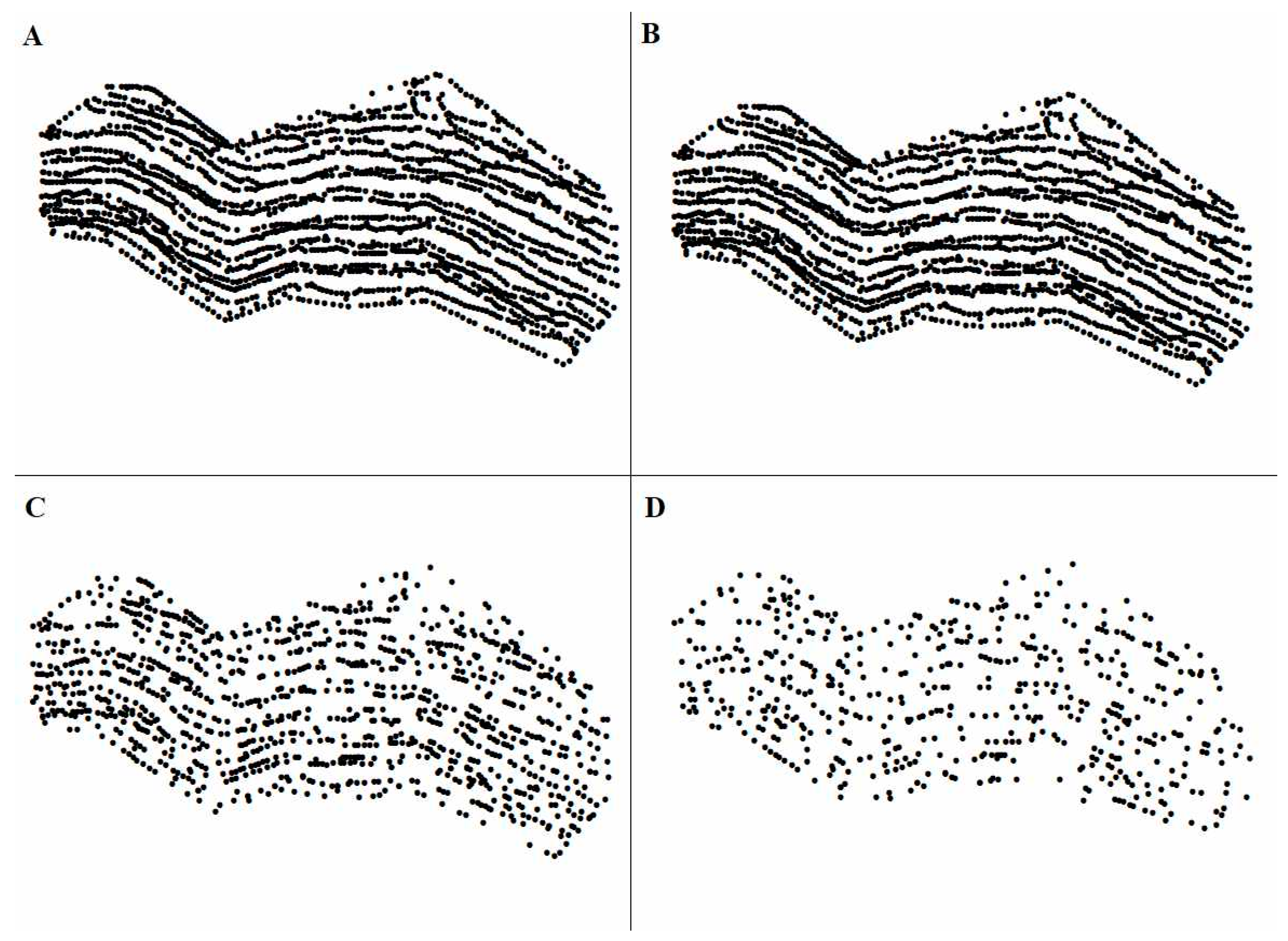
2.2. Data Collection and Preparation

Positional data points were collected with Trimble^® R8s real time kinetic geo-positioning system (RTK-GPS), by carrying a handheld receiver (“rover”) and establishing a base station for differential correction [13]. According to the manufacturer, the RTK-GPS has a theoretical horizontal accuracy of ±0.008 m + 1 ppm RMS, and a vertical accuracy of ±0.015 m + 1 ppm RMS [30]. However, a mean horizontal error of 0.014 m with standard deviation (SD) of 0.004 m, and a mean vertical error of 0.030 m with SD of 0.010 m were found under field conditions [4]. A total of 2722 data points were collected, over six hours, by walking transects across the site in a general east–west direction, at roughly 5 m intervals. The data collection was done on a clear sunny day to ensure minimum satellite distortion. At each point, coordinates (eastings, northings, and elevation) were recorded. All coordinates were georeferenced to the New Zealand Geodetic Datum 2000.

The train and test approach [31] was applied for quantitative evaluation of the GPS points. The collected data points were randomly partitioned into training (90%, n = 2440) and validation (10%, n = 282) datasets (Figure 2). The training dataset was randomly thinned by 25% (n = 1779), 50% (n = 1220), and 75% (n = 561) of its original point density (Figure 3 and

Table 1. Summary of elevations resulting from different training data thinning intensities.

Thinning (%)	Points	Elevation (m asl)				Point Density m−2
		Min.	Max.	Mean	St. Dev
0	2440	9.749	82.139	44.316	18.516	0.519
25	1830	9.748	82.139	44.580	18.295	0.389
50	1220	9.748	82.139	44.962	18.236	0.259
75	610	9.765	79.495	44.442	18.336	0.129

), which ranged from 0.519 points/m² to 0.129 points/m² (Table 1).

2.3. Interpolation Methods and Parameters

Interpolation methods have been intensively studied for producing DEMs. Kidner [32] and Torlegård, et al. [33] reported two major research areas: (1) developing new interpolation methods and (2) optimising the selection of existing interpolation methods. There are a number of existing geographic data interpolation methods with various different approaches and uses [21,23]. Lam [34] categorised interpolation as either point or aerial methods. Shi and Tian [35] suggested linear, non-linear, and hybrid methods, while other authors have suggested various physically-based interpolation methods [36,37,38,39]. However, Li and Heap [40] broadly classified all interpolation methods into two main forms, namely deterministic and stochastic methods. Stochastic methods integrate the concept of randomness, and provide both estimations and associated variances and uncertainties. In a broad sense, stochastic methods are based on statistical properties of the data. Deterministic interpolation methods create surfaces from measured points based on either similarity or a degree of smoothing [21]. As such, deterministic methods are considered the simplest and easiest to apply. Here, three deterministic methods were compared for their potential to interpolate an accurate digital elevation model from different intensities of thinned training data.

The selected interpolation methods, as described below, were applied across all training datasets, to create DEMs with spatial resolutions ranging from 0.5 m to 10 m, increasing in 0.5 m increments. In total, 20 DEMs were interpolated. All the interpolations were carried out with the default setting in ArcGIS 10.4.1 [41]. The training DEMs were then evaluated against the validation dataset to assess the degree of agreement between each DEM and measured elevation.

2.3.1. Inverse Distance Weighted (IDW)

Inverse distance weighted (IDW) interpolation is an automated technique [42], requiring very few parameters from the operators [43]. It is specifically suitable where the dataset range is narrow and other fitting techniques are heavily affected by errors. The process is highly flexible and allows for the estimation of datasets with a trend or anisotropy [44].

IDW estimates cell values through a linearly weighted combination of sample points, where the weight assigned to each sample point is the inverse of its distance from the cell being estimated [42]. The underlying assumption of IDW is that an unsampled cell’s value is a weighted average of known cells’ data in the local neighbourhood [44]. The surface being interpolated should be that of a locally dependent variable, and each cell’s value is estimated as

$$Z_j=\frac{{{\displaystyle \sum }}_{i=1}^n\frac{Z_i}{{\left(h_{ijk}+\delta \right)}^{\beta }}}{{{\displaystyle \sum }}_{i=1}^n\frac{1}{{\left(h_{ijk}+\delta \right)}^{\beta }}}$$

(1)

where Z_j is the unsampled location value, Z_i is the known cell’s value, β is the weight, and δ is the parameter. The separation distance h_ijk is measured by a three-dimensional Euclidian distance:

$$h_{ijk}=\sqrt{{\left(\Delta x\right)}^2+{\left(\Delta y\right)}^2+{\left(\Delta z\right)}^2}$$

(2)

where Δx and Δy are the distances between the unknown and known point according to the reference axes, respectively, and Δz refer to the height as the third point of measure.

2.3.2. Topo to Raster

Topo to raster (ANUDEM) interpolation is a morphological approach designed for scattered surface-specific point elevation data and stream line data. The input data may include point elevations, elevation contours, streamlines, sink data points, cliff lines, boundary polygons, lake boundaries, and data mask polygons. It attempts to take into account the special nature of the terrain surfaces, and the surface specific points that can be used for the sample terrain [45]. The topo to raster model is considered by many studies to produce hydrologically correct DEMs (e.g., [46,47]).

2.3.3. Natural Neighbors (NaN)

The natural neighbors (NaN) interpolation method was introduced by Sibson [48]. The model works by finding the nearest subset of samples for a given cell without a measured value, and then applies weights to the samples based on the proportional area they occupy [48]. In other words, it combines features from both nearest neighbours (NN) and triangular irregular network (TIN) interpolation methods. It starts with a triangulation of the data by Delaunay’s method, and then finds adjacent samples by Thiessen polygons. The value of an unknown cell is estimated by inserting and determining the point within a polygon. For each neighbour, the area of the portion of its original polygon that becomes incorporated in the tile of the new point is calculated [49]. This method is well known for its ability to interpolate scattered and unevenly distributed data [50].

2.4. Analysis

For evaluation purposes, a set of statistical calculations was carried out (

Table 2. Statistical metrics to assess interpolation quality.

Statistical features	Definitions
	N = umber of observations
	$O$ = observed value
	$\overline{O}$ = mean of observed value
	$P$ = predicted value
	${P^{\prime }}_i=P_i-\overline{O}$
	${O^{\prime }}_i=O_i-\overline{O}$
Ordinary least square regression	Slope
	Intercept
	r2 = coefficient of determination
Mean bias error (MBE)	$MBE=\frac{{{\displaystyle \sum }}_{i=1}^N(P_i-O_i)}{N}$
Root mean square error (RMSE)	$RMSE=\sqrt{\frac{{{\displaystyle \sum }}_{i=1}^N{(P_i-O_i)}^2}{N}}$
Mean absolute error (MAE)	$MAE=\frac{{{\displaystyle \sum }}_{i=1}^N|P_i-O_i|}{N}$
Model efficiency (EF)	$EF=1-\frac{{{\displaystyle \sum }}_{i=1}^N{(P_i-O_i)}^2}{{{\displaystyle \sum }}_{i=1}^N{(\overline{O}-O_i)}^2}$

), following Willmott [51], Vicente-Serrano, et al. [52], and Li and Heap [40] in an R statistical environment by using base packages [53]. These include the coefficient of determination (r²) from the ordinary least square (OLS) model; the bias of the model, as indicated by the intercept–slope pair; the mean bias error (MBE); the mean absolute error (MAE); and the root mean square error (RMSE). MAE and RMSE are the best overall measures for evaluating agreement between observed and predicted data [40,52,54]. Both are similar metrics, except the RMSE is more sensitive to extreme outliers, whereas MAE is less so. To overcome that sensitivity, we include model efficiency (EF), which is based on the relationship between observed and predicted mean deviations [55]. EF values closer to 1 specify model reliability.

In addition to statistical metrics, a subjective evaluation was also undertaken to evaluate the different interpolations. As Daly, et al. [56] highlighted, empirical knowledge can help to determine which method best reflects reality, so long as those methods produce reasonable statistical values. As a result, following the statistical evaluation, DEMs were visually assessed for their agreement with the original landscape.

3. Results

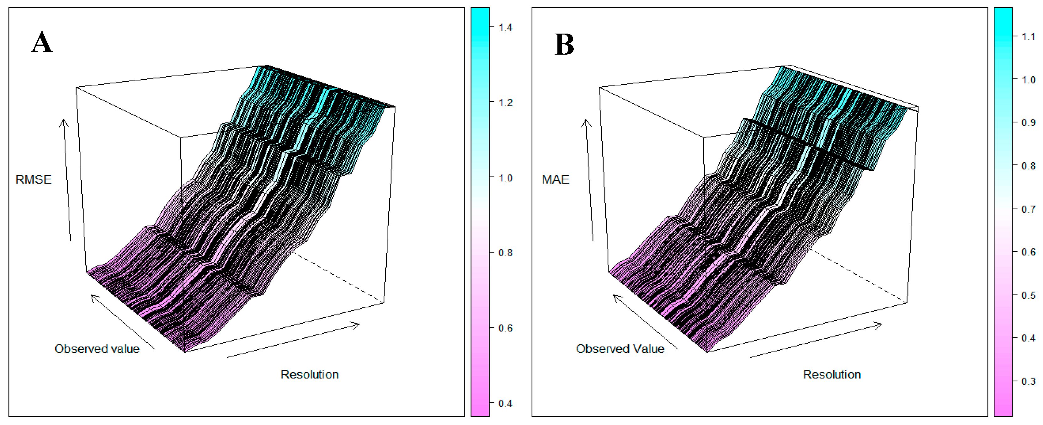
3.1. Digital Elevation Model Resolution Analysis

All the DEM resolutions yielded very high r² values, ranging from 0.9946–0.9995 (

Table 3. Results of statistical analysis for different digital elevation models (DEM) resolutions.

Resolution	r2	Slope	Intercept	RMSE (m)	MAE (m)	MBE (m)	EF
0.5	0.9995	1.0042	−0.2155	0.428	0.274	0.029	0.999
1	0.9994	1.0051	−0.2604	0.450	0.308	0.036	0.999
1.5	0.9994	1.0042	−0.2114	0.455	0.325	0.024	0.999
2	0.9993	1.0039	−0.2213	0.488	0.363	0.049	0.999
2.5	0.9992	1.0053	−0.2654	0.532	0.409	0.029	0.998
3	0.9991	1.0049	−0.2438	0.571	0.447	0.024	0.998
3.5	0.9989	1.0027	−0.1715	0.616	0.484	0.051	0.998
4	0.9989	1.0048	−0.2549	0.615	0.485	0.040	0.998
4.5	0.9987	1.0077	−0.3825	0.697	0.548	0.044	0.998
5	0.9984	1.0064	−0.3156	0.758	0.600	0.033	0.998
5.5	0.9982	1.0077	−0.3316	0.804	0.648	−0.009	0.997
6	0.998	1.0020	−0.1096	0.830	0.656	0.021	0.997
6.5	0.9976	1.0056	−0.2718	0.91	0.744	0.024	0.997
7	0.9974	1.0057	−0.3005	0.968	0.789	0.050	0.996
7.5	0.9966	1.0094	−0.4256	1.103	0.889	0.011	0.996
8	0.9965	1.0049	−0.1730	1.108	0.877	−0.044	0.995
8.5	0.9957	1.0032	−0.1151	1.228	0.991	−0.026	0.995
9	0.9953	1.0034	−0.0916	1.276	1.030	−0.060	0.994
9.5	0.9945	1.0030	−0.1725	1.384	1.107	0.040	0.994
10	0.9946	1.0062	−0.1957	1.380	1.088	−0.077	0.994

). The 0.5 m resolution produced the DEM surface with highest r² value (0.9995) and r² values decreased with a reduction in resolution, reaching 0.9946 at 10 m resolution. This result was reinforced by the RMSE and MAE being lowest for the 0.5 m resolution DEM (Table 3 and Figure 4), and increasing steadily from 0.429 m to 1.38 m and from 0.274 m to 1.088 m for the RMSE and MAE, respectively, at 10 m resolution. The MBE, which indicates the bias of the prediction, showed that at or below resolutions of 5 m the DEMs underestimated elevation slightly, whereas at coarser resolutions (specifically at 5.5 m, 8 m, 8.5 m, 9 m, and 10 m), the DEMs generally overestimated elevation. Moreover, the EF (0.999 > 0.994) for 0.5 m resolution was closer to 1 compared to lower resolutions, which indicates being in line with other findings, irrespective of any of the three selected methods.

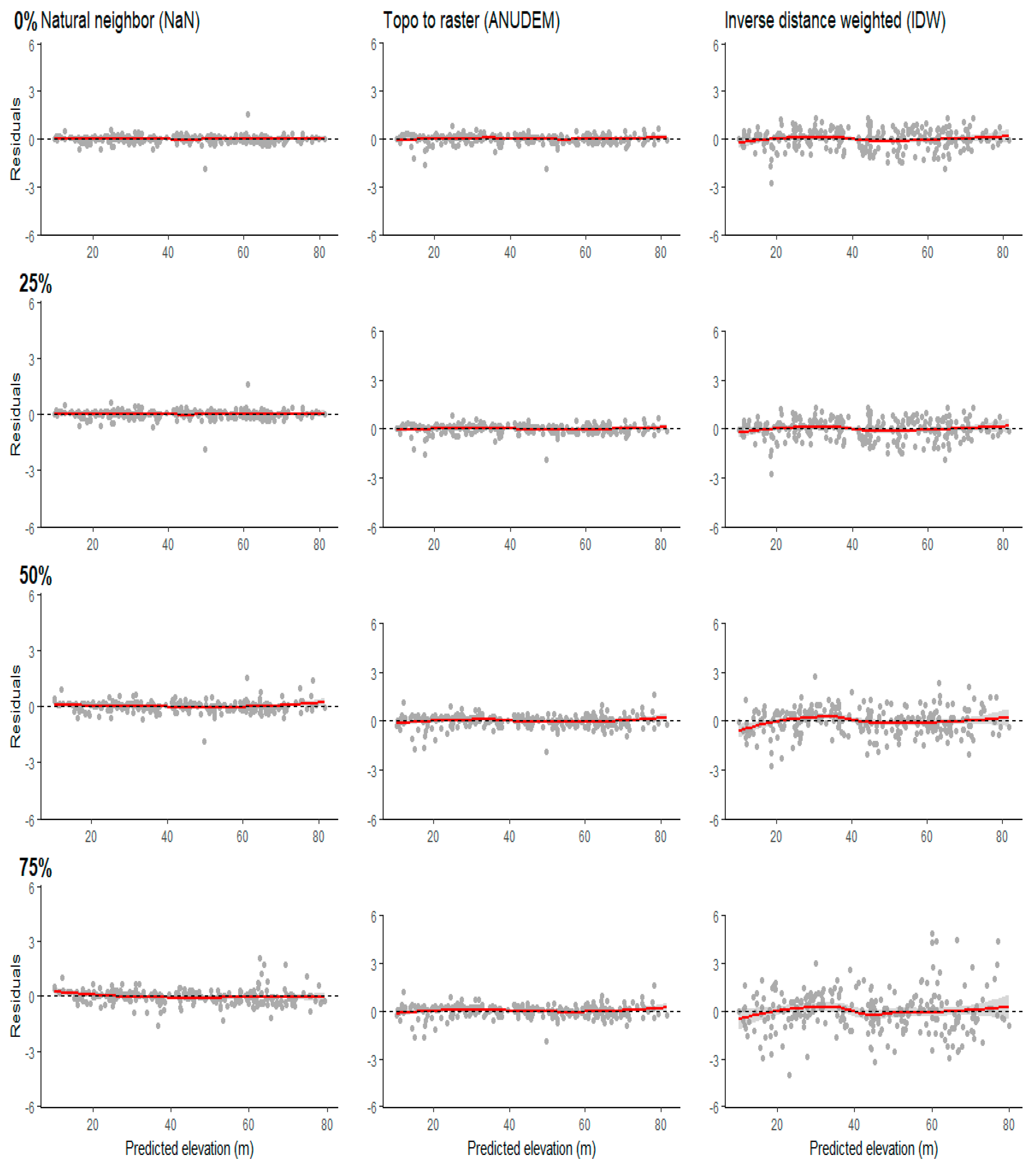
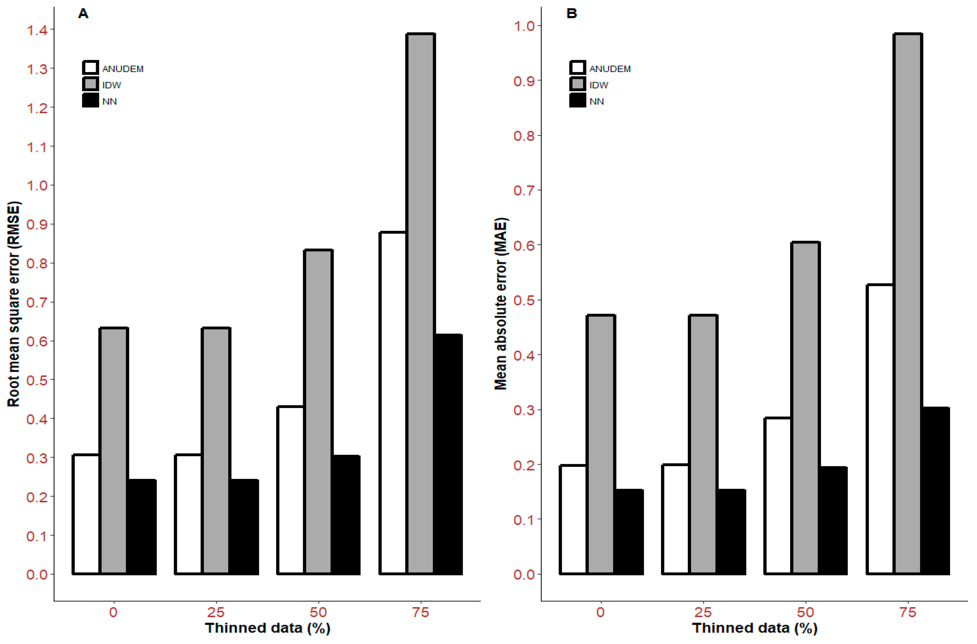
3.2. Interpolation Methods and Data Density

GPS points were thinned by 25%, 50%, and 75%, and interpolated into three DEMs with 0.5 m resolution, using each of the three different interpolation methods. Thinning had little effect on r² relative to the DEM produced from the complete set of data points (0% thinned) (

Table 4. Comparison of the three methods at 0.5 m resolution with different data densities.

Method	Thinning (%)	r2	Slope	Intercept	MBE
Natural Neighbour (NaN)	0	0.9995	1.004	−0.216	0.004
	25	0.9998	1.001	−0.090	0.004
	50	0.9997	1.003	−0.140	−0.015
	75	0.999	1.009	−0.370	−0.059
Inverse Distance Weighting (IDW)	0	0.9989	1.004	−0.269	0.059
	25	0.9989	1.004	−0.269	0.059
	50	0.9982	1.014	−0.730	0.116
	75	0.9952	1.027	−1.238	0.029
Topo to Raster (ANUDEM)	0	0.9998	1.005	−0.284	0.024
	25	0.9998	1.005	−0.282	0.022
	50	0.9996	1.010	−0.489	0.028
	75	0.9984	1.024	−1.046	−0.044

). Even with 75% thinning, the r² values only decreased to 0.999, 0.9952, and 0.9984 for the natural neighbor (NaN), inverse distance weighting (IDW), and Topo to raster (ANUDEM) methods, respectively. NaN had the lowest levels of bias at 25% (MBE = 0.004 m) and 50% (MBE = −0.015 m), while at 75% thinning, IDW exhibited the least bias (MBE = 0.029 m).

Given the high r² values, it is unsurprising that generally the observed and predicted values were in agreement (Figure 5). The observed and predicted values of the data points were slightly more scattered in the DEM, interpolated using IDW. Figure 5 also shows that the spread of the residuals increased when elevation data were thinned by 75% prior to DEM interpolation.

RMSE and MAE data provide better opportunities to discriminate between different interpolation algorithms with thinned data. IDW yielded the highest RMSE and MAE, irrespective of the level of data thinning applied (Figure 6). For IDW, RMSE ranged between 0.631 m and 1.388 m, and MAE ranged between 0.471 m and 0.984 m. In contrast, NaN and ANUDEM interpolations resulted in lower RMSE and MAE values at all thinning intensities. RMSE ranged between 0.239 m and 0.614 m and between 0.305 m and 0.877 m for NaN and ANUDEM, respectively, while MAE ranged between 0.152 m and 0.301 m and between 0.197 m and 0.526 m. Irrespective of interpolation algorithm, RMSE and MAE remained reasonably consistent until 75% thinning, when there was a large increase in both metrics. At 75% thinning, the density of the points used to interpolate the DEM was only 0.129 points m⁻², compared with 0.519 points m⁻² in the un-thinned data.

In addition to quantitative analyses, a visual inspection was carried out on the DEMs produced by the three interpolation methods. It was found that the IDW produced a less reliable surface, with a lot of abnormalities (Figure 7(C0–C3)). In contrast, the NaN and ANUDEM produced more consistent and representative DEM surfaces. Moreover, among the two, ANUDEM interpolated the DEM surface, both with consistency and reliability, in relation to the original surface (Figure 7(B0–B3)). It resembled reality more closely, where NaN produced a surface that was overly smooth and unrealistic (Figure 7(A0–A3)). With greater elevation data density, the surface better resembled the original natural surface, showing features like mounds or gullies—whereas, with the reduction of elevation data points through thinning, the surface was rendered relatively smoothly, and topographic features that were visible with higher data densities were obscured. For example, a gully on the site was virtually invisible with the lowest data density (i.e., 75% thinning) (Figure 7(A3,B3,C3)).

4. Discussion

4.1. An Alternate Data Source

The GNSS-surveyed elevation point data can be used to produce a high-resolution DEM. Though aerial laser scanning data are commonly used for this purpose, their shortcomings may preclude their use in some instances. In contrast, collecting elevation data via GNSS surveys is inexpensive and easy to undertake, often with little or no specialist skill. The data density of ALS yields high accuracy and resolution [57,58]. However, depending on the desired DEM resolution, the high point density associated with ALS data may not be needed [57], suggesting that the relatively low elevation data density achievable with a GNSS approach may be appropriate under some conditions; however, this will depend on the required resolution and the interpolation used to generate the DEM.

4.2. Optimal Resolution

Spatial resolution is important for DEMs, as many other surfaces can be derived from it. Errors in a DEM are perpetuated through to derived aspect, slope, hill-shade, and surface curvature surfaces, amongst many others. Moreover, DEMs are critical in their role for normalising digital surface models. In this study, errors in the DEM were minimized by increasing spatial resolution from 10 m to 0.5 m. This finding is in line with previous research showing that DEMs interpolated from LiDAR point clouds had accuracy proportional to spatial resolution [59,60,61]. Although those results were based on LiDAR data, which typically has much greater point density than the point density achieved with the GNSS approach, in this study, the underlying theory remains the same.

4.3. Influencers of Digital Elevation Model Quality

The question of resolution and DEM accuracy is also dependent on the characteristics of the surface being modelled [26,59,62]. Flat surfaces can be interpolated accurately even with relatively few elevation points due to topographic homogeneity. In contrast, surfaces that are topographically heterogeneous are likely to require greater point density and higher resolution, in order to capture small undulations or other features in the landscape.

Data density and distribution have also been shown to influence interpolation quality [22,63]. The present study clearly shows that elevation point density influenced DEM quality. At low densities, a small number of data points were used for interpolation, creating a generalized surface; this was because most of the deterministic approaches are mainly based on some simple mathematical functions [22]. Li and Heap [23] reported that data distribution had a greater effect, relative to data density, on the quality of the DEM produced.

On the contrary, it is not suitable to produce high-resolution DEMs from sparse data, as the surface will be shaped by the proliferated interpolator and interpolation artefacts [58,64,65], as well as the resolution constraints designated by the data density [66]. For this study, all the data were collected in a way that was assumed to give an evenly distributed dataset. Hence, the effect of distribution was not tested explicitly. Moreover, the selection of validation points, thinning, and study site characteristics would have resulted in some spatial variation in point distribution. Firstly, the validation points had high positive spatial correlation with the training dataset as they were not independently collected and lying in line with each other. Secondly, even though the thinning routine was performed in a randomised manner, minor clustering may have influenced the results. Thirdly, the study site was relatively small. Hence, it is expected that the results are site specific and could vary with changes in site or surface structure. For example, if the site were more rugged than the one used here, a higher level of error could be expected.

4.4. Deterministic Interpolation Method

The interpolation method is important for the accuracy of the interpolated digital elevation model, because interpolation can vary with the nature of the surface terrain and spatial structure [26,62,67]. In the present study, though, ANUDEM and NaN had similar quantitative metrics: ANUDEM produced a more realistic and consistent DEM, relative to the NaN interpolation. NaN is mostly used in cases where there is a need to have a geo-morphologically smooth surface [68], whereas ANUDEM tends to be useful where well-defined drainage and major topographic features exist [45]. It is important to note that there is no single optimal interpolation method, but rather many methods optimized by matching them with particular end uses of the DEM [69]. This is further supported by Arun [62] and Kienzle [59], who stated that the interpolation method is mostly chosen based on the purpose and focus of the research. The implication of this research and previous studies is the importance of testing various interpolation algorithms for individual sites, in order to create a guide through the process of obtaining an optimised one.

5. Summary and Conclusions

This study evaluated the quality of digital elevation models interpolated from elevation data acquired from a differentially corrected GNSS (RTK-GPS) receiver. Three interpolation methods (NN, IDW, and ANUDEM) were compared, as was the influence of different spatial resolutions and data densities. With dense and regularly distributed data, a high-resolution DEM (0.5 m) was interpolated, with RMSE value 0.428 m and MSE value 0.274 m. Thinning the elevation point data by 25% or even 50% had minimal effect on the DEM quality. Despite similar quality from a quantitative perspective, ANUDEM performed better than NN- and IDW-interpolated DEMs from a qualitative perspective. In this study, the use of quantitative and qualitative approaches for judging DEM quality resulted in a better decision.

LiDAR data acquisition has become the standard approach for collecting point data to interpolate high-resolution ground and above-ground surfaces (e.g., canopy height model). LiDAR acquisition is generally only cost-effective over large contiguous areas of land. The present results are promising for applications where it is unfeasible to acquire LiDAR data. The RMSE and MAE values are higher than those from LiDAR studies [70], but are within an order of magnitude, and therefore comparable. In conclusion, the interpolation of data collected via GNSS surveys can yield accurate digital elevation models. This method should be considered alongside LiDAR data interpolation as a viable means of generating topographic surfaces, especially in cases where study areas are small and easily accessible. In these areas, the GNSS approach can provide a low-cost, efficient, and effective solution for DEM creation.

References

1. Peralvo, M.; Maidment, D. Influence of DEM interpolation methods in drainage analysis. Gis Hydro 2004, 4. [Google Scholar]
2. Liu, X. Airborne lidar for DEM generation: Some critical issues. Prog. Phys. Geogr. Earth Environ. 2008, 32, 31–49. [Google Scholar]
3. Vaze, J.; Teng, J. High resolution lidar DEM—How good is it? Model. Simul. 2007, 692–698. [Google Scholar]
4. Koci, J.; Jarihani, B.; Leon, J.X.; Sidle, R.; Wilkinson, S.; Bartley, R. Assessment of uav and ground-based structure from motion with multi-view stereo photogrammetry in a gullied savanna catchment. ISPRS Int. J. Geo-Inf. 2017, 6, 328. [Google Scholar] [CrossRef]
5. Traganos, D.; Poursanidis, D.; Aggarwal, B.; Chrysoulakis, N.; Reinartz, P. Estimating satellite-derived bathymetry (SDB) with the google earth engine and sentinel-2. Remote Sens. 2018, 10, 859. [Google Scholar] [CrossRef]
6. Kodors, S. Point distribution as true quality of lidar point cloud. Balt. J. Mod. Comput. 2017, 5, 362–378. [Google Scholar] [CrossRef]
7. Morgenroth, J.; Visser, R. Uptake and barriers to the use of geospatial technologies in forest management. N. Z. J. For. Sci. 2013, 43, 16. [Google Scholar] [CrossRef] [Green Version]
8. Kurz, T.H.; Buckley, S.J.; Howell, J.A.; Schneider, D. In close range hyperspectral and lidar data integration for geological outcrop analysis. In Proceedings of the 2009 First Workshop on Hyperspectral Image and Signal Processing: Evolution in Remote Sensing, Grenoble, France, 26–28 August 2009; pp. 1–4. [Google Scholar]
9. Tagarakis, A.C.; Koundouras, S.; Fountas, S.; Gemtos, T. Evaluation of the use of lidar laser scanner to map pruning wood in vineyards and its potential for management zones delineation. Precis. Agric. 2018, 19, 334–347. [Google Scholar] [CrossRef]
10. Yu, B.; Liu, H.; Wu, J.; Hu, Y.; Zhang, L. Automated derivation of urban building density information using airborne lidar data and object-based method. Landsc. Urban Plan. 2010, 98, 210–219. [Google Scholar] [CrossRef]
11. Parkinson, B.W.; Enge, P.; Axelrad, P.; Spilker, J.J., Jr. Global Positioning System: Theory and Applications, Volume II; American Institute of Aeronautics and Astronautics: Washington, DC, USA, 1996. [Google Scholar]
12. Pick, J. A case-study analysis of costs and benefits of geographic information systems: Relationships to firm size and strategy. In Proceedings of the 12th Americas Conference on Information Systems (AMCIS 2006), Acapulco, Mexico, 4–6 August 2006; Curran Associates, Inc.: Red Hook, NY, USA, 2007. [Google Scholar]
13. Hofmann-Wellenhof, B.; Lichtenegger, H.; Collins, J. Global Positioning System: Theory and Practice; Springer Science & Business Media: Dordrecht, The Netherlands, 2012. [Google Scholar]
14. Groves, P.D. Principles of Gnss, Inertial, and Multisensor Integrated Navigation Systems; Artech House: Norwood, MA, USA, 2013. [Google Scholar]
15. Neményi, M.; Mesterházi, P.Á.; Pecze, Z.; Stépán, Z. The role of GIS and GPS in precision farming. Comput. Electron. Agric. 2003, 40, 45–55. [Google Scholar] [CrossRef]
16. Olivera, A.; Visser, R.; Acuna, M.; Morgenroth, J. Automatic GNSS-enabled harvester data collection as a tool to evaluate factors affecting harvester productivity in a Eucalyptus spp. Harvesting operation in Uruguay. Int. J. For. Eng. 2016, 27, 15–28. [Google Scholar] [CrossRef]
17. Gao, J. Towards accurate determination of surface height using modern geoinformatic methods: Possibilities and limitations. Prog. Phys. Geogr. Earth Environ. 2007, 31, 591–605. [Google Scholar] [CrossRef]
18. Yao, H.; Clark, R.L. Evaluation of sub-meter and 2 to 5 meter accuracy GPS receivers to develop digital elevation models. Precis. Agric. 2000, 2, 189–200. [Google Scholar] [CrossRef]
19. Gong, J.; Li, Z.; Zhu, Q.; Sui, H.; Zhou, Y. Effects of various factors on the accuracy of dems: An intensive experimental investigation. Photogramm. Eng. Remote Sens. 2000, 66, 1113–1117. [Google Scholar]
20. Chaplot, V.; Darboux, F.; Bourennane, H.; Leguédois, S.; Silvera, N.; Phachomphon, K. Accuracy of interpolation techniques for the derivation of digital elevation models in relation to landform types and data density. Geomorphology 2006, 77, 126–141. [Google Scholar] [CrossRef]
21. Li, J.; Heap, A.D. A Review of Spatial Interpolation Methods for Environmental Scientists; Geosciene Australia: Canberra, Australia, 2008. [Google Scholar]
22. Erdogan, S. A comparision of interpolation methods for producing digital elevation models at the field scale. Earth Surf. Process. Landf. 2009, 34, 366–376. [Google Scholar] [CrossRef]
23. Li, J.; Heap, A.D. A review of comparative studies of spatial interpolation methods in environmental sciences: Performance and impact factors. Ecol. Inform. 2011, 6, 228–241. [Google Scholar] [CrossRef]
24. Mitas, L.; Mitasova, H. Spatial interpolation. In Geographical Information Systems: Principles, Techniques, Management and Applications; Wiley: New York, NY, USA, 1999; Volume 1, pp. 481–492. [Google Scholar]
25. Robinson, T.P.; Metternicht, G. Testing the performance of spatial interpolation techniques for mapping soil properties. Comput. Electron. Agric. 2006, 50, 97–108. [Google Scholar] [CrossRef]
26. Zimmerman, D.; Pavlik, C.; Ruggles, A.; Armstrong, M.P. An experimental comparison of ordinary and universal kriging and inverse distance weighting. Math. Geol. 1999, 31, 375–390. [Google Scholar] [CrossRef]
27. Amjad, M.; Ali, M.Z.; Shafique, M. Impact of DEM resolution and accuracy on remote sensing and topographic dem derived topographic attributes and drainage pattern. J. Himal. Earth Sci. 2016, 49, 109–117. [Google Scholar]
28. Habtezion, N.; Tahmasebi Nasab, M.; Chu, X. How does DEM resolution affect microtopographic characteristics, hydrologic connectivity, and modelling of hydrologic processes? Hydrol. Process. 2016, 30, 4870–4892. [Google Scholar] [CrossRef]
29. NIWA. Overview of New Zealand Climate. Available online: https://www.niwa.co.nz/education-and-training/schools/resources/climate/overview (accessed on 26 August 2015).
30. Trimble. Trimble r8s GNSS System; Trimble Inc.: Sunnyvale, CA, USA, 2017. Available online: https://geospatial.trimble.com/products-and-solutions (accessed on 13 June 2018).
31. Miller, J. Incorporating spatial dependence in predictive vegetation models: Residual interpolation methods. Prof. Geogr. 2005, 57, 169–184. [Google Scholar] [CrossRef]
32. Kidner, D.B. Higher-order interpolation of regular grid digital elevation models. Int. J. Remote Sens. 2003, 24, 2981–2987. [Google Scholar] [CrossRef]
33. Torlegård, K.; Östman, A.; Lindgren, R. A comparative test of photogrammetrically sampled digital elevation models. Photogrammetria 1986, 41, 1–16. [Google Scholar] [CrossRef]
34. Lam, N.S.-N. Spatial interpolation methods: A review. Am. Cartogr. 1983, 10, 129–150. [Google Scholar] [CrossRef]
35. Shi, W.Z.; Tian, Y. A hybrid interpolation method for the refinement of a regular grid digital elevation model. Int. J. Geogr. Inf. Sci. 2006, 20, 53–67. [Google Scholar] [CrossRef]
36. Grimaldi, S.; Teles, V.; Bras, R.L. Sensitivity of a physically based method for terrain interpolation to initial conditions and its conditioning on stream location. Earth Surf. Process. Landf. 2004, 29, 587–597. [Google Scholar] [CrossRef]
37. Niemann, J.D.; Bras, R.L.; Veneziano, D. A physically based interpolation method for fluvially eroded topography. Water Resour. Res. 2003, 39. [Google Scholar] [CrossRef] [Green Version]
38. Grimaldi, S.; Teles, V.; Bras, R.L. Preserving first and second moments of the slope area relationship during the interpolation of digital elevation models. Adv. Water Resour. 2005, 28, 583–588. [Google Scholar] [CrossRef]
39. Sandmeier, S.; Itten, K.I. A physically-based model to correct atmospheric and illumination effects in optical satellite data of rugged terrain. IEEE Trans. Geosci. Remote Sens. 1997, 35, 708–717. [Google Scholar] [CrossRef]
40. Li, J.; Heap, A.D. Spatial interpolation methods applied in the environmental sciences: A review. Environ. Model. Softw. 2014, 53, 173–189. [Google Scholar] [CrossRef]
41. ESRI. ArcGIS Release 10.1. ESRI: Redlands, CA, USA, 2012.
42. Philip, G.; Watson, D.F. A precise method for determining contoured surfaces. APPEA J 1982, 22, 205–212. [Google Scholar] [CrossRef]
43. Hessl, A.; Miller, J.; Kernan, J.; Kenum, D.; McKenzie, D. Mapping paleo-fire boundaries from binary point data: Comparing interpolation methods. Prof. Geogr. 2007, 59, 87–104. [Google Scholar] [CrossRef]
44. Garnero, G.; Godone, D. Comparisons between different interpolation techniques. In Proceedings of the International Archives of the Photogrammetry, Remote Sensing and Spatial Information Sciences XL-5 W, Padua, Italy, 27–28 February 2013; Volume 3, pp. 27–28. [Google Scholar]
45. Hutchinson, M. A new procedure for gridding elevation and stream line data with automatic removal of spurious pits. J. Hydrol. 1989, 106, 211–232. [Google Scholar] [CrossRef]
46. Curebal, I.; Efe, R.; Ozdemir, H.; Soykan, A.; Sönmez, S. Gis-based approach for flood analysis: Case study of keçidere flash flood event (Turkey). Geocarto Int. 2016, 31, 355–366. [Google Scholar] [CrossRef]
47. Salari, A.; Zakaria, M.; Nielsen, C.C.; Boyce, M.S. Quantifying tropical wetlands using field surveys, spatial statistics and remote sensing. Wetlands 2014, 34, 565–574. [Google Scholar] [CrossRef]
48. Sibson, R. A brief description of natural neighbor interpolation. In Interpreting Multivariate Data; John Wiley & Sons: Hoboken, NJ, USA, 1981; pp. 21–36. [Google Scholar]
49. Webster, R.; Oliver, M. Geostatistics for Environmental Scientists (Statistics in Practice); Wiley: Hoboken, NJ, USA, 2001. [Google Scholar]
50. Ledoux, H.; Gold, C. An Efficient Natural Neighbour Interpolation Algorithm for Geoscientific Modelling; Springer: Berlin/Heidelberg, Germany, 2005; pp. 97–108. [Google Scholar]
51. Willmott, C.J. On the validation of models. Phys. Geogr. 1981, 2, 184–194. [Google Scholar]
52. Vicente-Serrano, S.M.; Saz-Sánchez, M.A.; Cuadrat, J.M. Comparative analysis of interpolation methods in the middle Ebro Valley (Spain): Application to annual precipitation and temperature. Clim. Res. 2003, 24, 161–180. [Google Scholar] [CrossRef]
53. R Core Team. R: A Language and Environment for Statistical Computing; R Core Team: Vienna, Austria, 2014; Available online: http://www.R-project.org (accessed on 5 June 2018).
54. Willmott, C.J. Some comments on the evaluation of model performance. Bull. Am. Meteorol. Soc. 1982, 63, 1309–1313. [Google Scholar] [CrossRef]
55. Greenwood, D.J.; Neeteson, J.J.; Draycott, A. Response of potatoes to n fertilizer: Dynamic model. Plant Soil 1985, 85, 185–203. [Google Scholar] [CrossRef]
56. Daly, C.; Gibson, W.P.; Taylor, G.H.; Johnson, G.L.; Pasteris, P. A knowledge-based approach to the statistical mapping of climate. Clim. Res. 2002, 22, 99–113. [Google Scholar] [CrossRef] [Green Version]
57. Anderson, E.S.; Thompson, J.A.; Crouse, D.A.; Austin, R.E. Horizontal resolution and data density effects on remotely sensed lidar-based DEM. Geoderma 2006, 132, 406–415. [Google Scholar] [CrossRef]
58. Liu, X.; Zhang, Z.; Peterson, J.; Chandra, S. The effect of lidar data density on DEM accuracy. In Proceedings of the International Congress on Modelling and Simulation (MODSIM07), Christchurch, New Zealand, 10–13 Decembert 2017; Modelling and Simulation Society of Australia and New Zealand Inc.: Perth, WA, Australia, 2007; pp. 1363–1369. [Google Scholar]
59. Kienzle, S. The effect of DEM raster resolution on first order, second order and compound terrain derivatives. Trans. GIS 2004, 8, 83–111. [Google Scholar] [CrossRef]
60. Ouma, Y. Evaluation of multiresolution digital elevation model (DEM) from real-time kinematic GPS and ancillary data for reservoir storage capacity estimation. Hydrology 2016, 3, 16. [Google Scholar] [CrossRef]
61. Thomas, I.A.; Jordan, P.; Shine, O.; Fenton, O.; Mellander, P.E.; Dunlop, P.; Murphy, P.N.C. Defining optimal DEM resolutions and point densities for modelling hydrologically sensitive areas in agricultural catchments dominated by microtopography. Int. J. Appl. Earth Obs. Geoinf. 2017, 54, 38–52. [Google Scholar] [CrossRef]
62. Arun, P.V. A comparative analysis of different DEM interpolation methods. Egypt. J. Remote Sens. Space Sci. 2013, 16, 133–139. [Google Scholar]
63. Guo, Q.; Li, W.; Yu, H.; Alvarez, O. Effects of topographic variability and lidar sampling density on several dem interpolation methods. Photogramm. Eng. Remote Sens. 2010, 76, 701–712. [Google Scholar] [CrossRef]
64. Albani, M.; Klinkenberg, B.; Andison, D.W.; Kimmins, J.P. The choice of window size in approximating topographic surfaces from digital elevation models. Int. J. Geogr. Inf. Sci. 2004, 18, 577–593. [Google Scholar] [CrossRef]
65. Florinsky, I.V. Errors of signal processing in digital terrain modelling. Int. J. Geogr. Inf. Sci. 2002, 16, 475–501. [Google Scholar] [CrossRef]
66. Florinsky, I.V. Combined analysis of digital terrain models and remotely sensed data in landscape investigations. Prog. Phys. Geogr. Earth Environ. 1998, 22, 33–60. [Google Scholar] [CrossRef]
67. Tan, Q.; Xu, X. Comparative analysis of spatial interpolation methods: An experimental study. Sens. Transducers 2014, 165, 155–163. [Google Scholar]
68. Bobach, T.; Umlauf, G. Natural neighbor concepts in scattered data interpolation and discrete function approx-imation. In Visualization of Large and Unstructured Data Sets; GI Digital Library: Kowloon, Hong Kong, China, 2008. [Google Scholar]
69. Li, X.; Cheng, G.; Lu, L. Comparison of spatial interpolation methods. Adv. Earth Sci. 2000, 3, 3. [Google Scholar]
70. Hodgson, M.E.; Bresnahan, P. Accuracy of airborne lidar-derived elevation. Photogramm. Eng. Remote Sens. 2004, 70, 331–339. [Google Scholar] [CrossRef]
Figure 1. Location of the experimental site. Aerial imagery overlaid on a hillshade model.
Ijgi 07 00300 g001
Figure 2. Layout of the collected data points.
Ijgi 07 00300 g002
Figure 3. Training points were thinned by (A) 0%, (B) 25%, (C) 50%, and (D) 75%.
Ijgi 07 00300 g003
Figure 4. Effect of resolution at each observation point by (A) RMSE (root mean square error) and (B) MAE (mean absolute error).
Ijgi 07 00300 g004
Figure 5. Residuals plotted against predicted elevation (m) for different models and levels of data thinning. Red line shows the model prediction trend.
Ijgi 07 00300 g005
Figure 6. Comparison of three interpolation method in regards of different data density: (A) root mean square error (RMSE) and (B) mean absolute error (MAE).
Ijgi 07 00300 g006
Figure 7. Hillshade surfaces produced from DEMs interpolated by (A) nearest neighbor, (B) ANUDEM, and (C) IDW methods. Numbers 0 to 3 represent 0%, 25%, 50%, and 75% elevation data thinning prior to DEM interpolation.
Ijgi 07 00300 g007