Autonomous Point Cloud Acquisition of Unknown Indoor Scenes

Abstract

This paper presents a methodology for the automatic selection of heuristic scanning positions in unknown indoor environments. The surveying is carried out by a robotic system following a stop-and-go procedure. Starting with a random scan position in the room, the point cloud is discretized in voxels and they are submitted to a two-step classification and are labelled as occupied, occluded, empty, window, door, or exterior based on a visibility analysis. The main objective of the methodology is to obtain a complete point cloud of the indoor space and accordingly, the next best position is the scan position minimizing occluded voxels. Because the method locates doors and windows, the room can be delimited and the scan can continue for adjacent rooms. This approach has been tested in a real case study, in which three scans were developed.

1. Introduction

Nowadays, with increased computing capacity due to advances in the field of computer science, the use of three-dimensional (3D) information has grown and spread to multiple fields, from the cinematographic industry to the medical industry. The sensors used to obtain 3D information, such as cameras and laser scanners, have greatly improved in range, precision and price in recent years, which makes it a widely used technology today.

Undoubtedly one of the fields that most benefits from this technology is architecture, engineering and construction (AEC). Quality management and control processes have gained increasing attention in this field. An effective and systematic dimensional and quality assessment of as-built construction components with planned works is essential for the timely and successful completion of construction projects, thereby saving cost.

Dimensional analysis of construction elements is traditionally based on the use of remote sensing instruments such as distanciometers or total stations. Although these instruments are highly accurate, the procedure is very time-consuming [1,2,3]. Their use in some scenes is moving to laser scanning devices, which are being increasingly adopted as default instruments for the collection of 3D data in large-scale civil infrastructures [4] and cultural heritage sites [5,6].

Point clouds are composed of massive amounts of raw data and have to be processed in order to extract useful information for the applications they are intended to serve. For progress-tracking analysis in construction, building components have to be recognized in the point cloud and parameterized. Bosché et al. [7] used point clouds to evaluate flatness defects in surfaces during the construction of a building. Díaz-Vilariño et al. [8] presented a methodology for detecting and segmenting round and rectangular cross-section columns in as-built buildings from point clouds. A similar approach was evaluated by Bueno et al. [9] under different conditions of quality and completeness.

In addition to laser point density and accuracy, data completeness is an important aspect of point cloud quality [10] and, at the same time, one of the major drawbacks of indoor point cloud acquisition, because indoor spaces are typically highly occluded. Therefore, the acquisition should be planned in a way that obtains full coverage of the scene while avoiding major occlusions [11].

All this makes automating scanning and modelling processes especially important. To achieve correct modelling from the 3D information of an interior environment [12,13,14,15,16,17] the occluded space must be minimized.

The survey process of indoor scenes can be addressed from two different perspectives. On the one hand, data can be acquired in a static way by placing the sensor in different positions [18,19]. Data must be combined and registered in the same coordinate system to obtain the complete model of the scene. On the other hand, the use of mobile mapping systems enables the collection of 3D data continuously [20,21]. These systems are based on the 3D positioning of the sensor together with 2D laser scanning.

The planning and optimization of scans is still an active research line, especially when the scanning is performed by autonomous robots. In this paper, we present a method for total automation of the scanning of rooms from which we have no previous information. This method must ensure that we obtain all the desired 3D information safely and quickly, using a robotic system that carries the laser scanner and does the survey using a stop-and-go procedure.

The search for these optimal scanning positions is known as the next best view (NBV) problem. This topic has been addressed for many years and it consists of calculating optimal scanning positions. Connolly et al. [22] in 1985 used partial octree models to determine the “best” next view. Several methods have been used to solve this problem. Surmann et al. [23] simplified the geometry of a room to a 2D map, using lines that represent the walls for selection of the NBV. Grabowski et al. [24] defined a region of interest (ROI) that is used for calculating the NBV. The most common solution is to discretize the space of study using a 3D grid. In many cases, instead of an octree model, a simple voxelization is used, in which each voxel is classified as empty, occupied, or occluded [25,26]. Another problem that arises is delimiting the study area. Adán et al. [27] used a projection of the points belonging to the ceiling to delimit the study area. Usually, as in Prieto et al. [28], an ICP (Iterative Closest Point) algorithm is used for fine registration of point clouds.

Robots require an understanding of the environment to be able to move in it. When the scene is not known, positions should be determined from an analysis of the scene. Because the objective of this paper is the optimal acquisition of an unknown indoor scene, the next pose of the robot is the next best position in terms of data completeness. The space is discretized in voxels and they are classified into empty, occupied, or occluded. In addition, windows and doors are recognized in order to enable acquisition of adjacent rooms. The geometry of the study room is used for fine registration of consecutive point clouds.

The main innovations introduced in the methodology presented below are the introduction of three new types of voxels (window, door and out), locating the doors and windows of the room using a simple and fast method and using them to delimit the room, in addition to the calculation of the NBV giving depth to the occluded areas.

The manuscript is organized as follows. Section 2 describes the proposed methodology. Section 3 reports the results obtained from applying the methodology to a real case study composed of several rooms and a discussion of those results. Finally, Section 4 concludes this work.

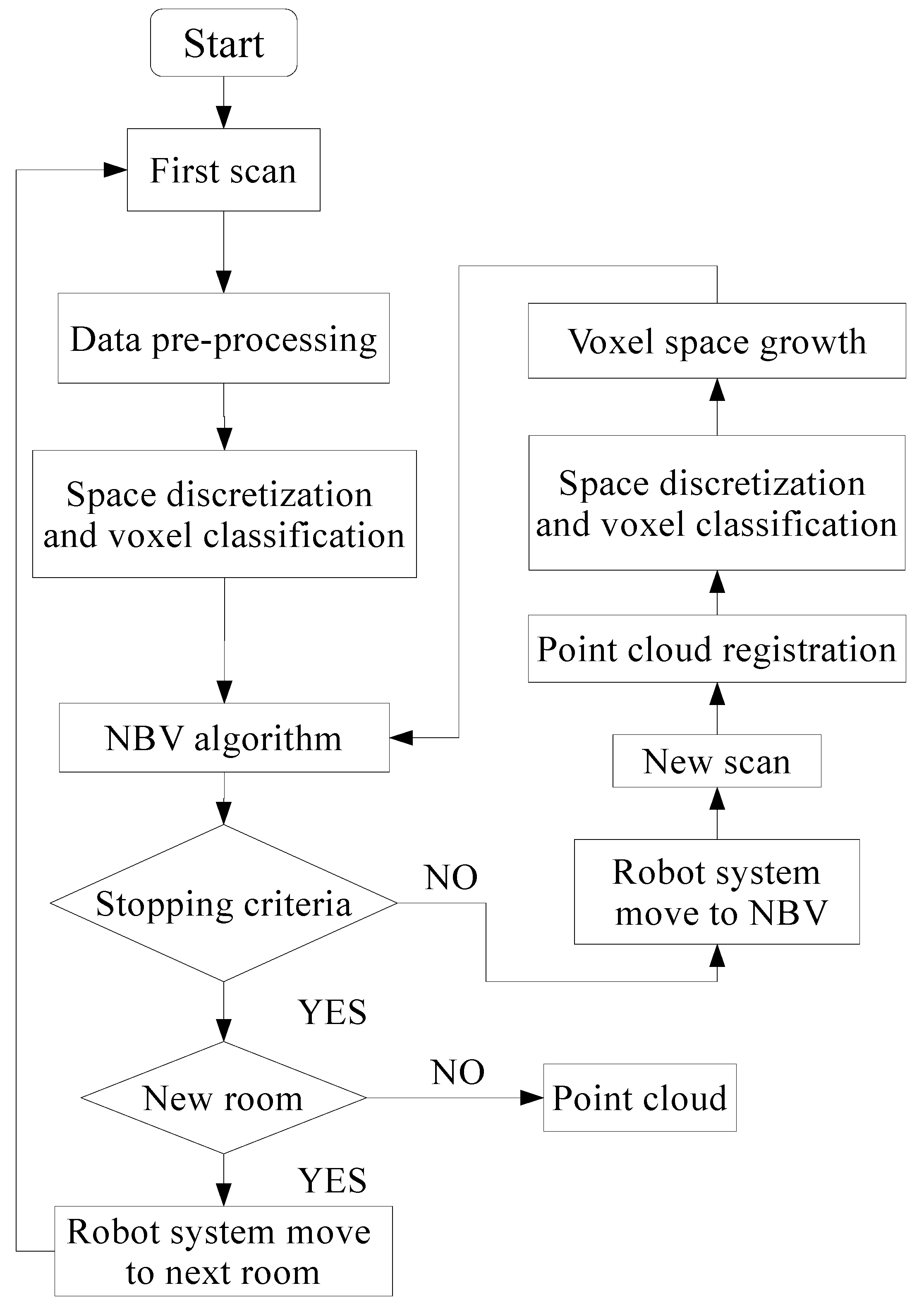
2. Methodology

The methodology consists of data collection and pre-processing, two-step voxel classification, next best view (NBV) computation, scan registration and voxel growing. The general workflow of this methodology is summarized in Figure 1.

To develop the methodology, the Robotnik Guardian UGV (Unmanned Ground Vehicle) was simulated [29]. To this end, the system features provided by the fabricant were used, emulating the assembly of this system with the Faro Focus 3D X330 (Faro Technologies Inc., FL, USA), which was used to scan the study room. This UGV has a payload of 50 kg and an autonomy of 3 h, therefore, problems of payload and autonomy have not been taken into account. A similar system was used in Prieto et al. [28] and in Adán et al. [27], in which they used a previous version of this UGV in conjunction with a Riegl 3D laser scanner. This system uses simultaneous localization and mapping (SLAM) algorithms to be able to move autonomously in indoor environments. Therefore, we will focus on the calculation of this optimal scanning position, which would be communicated to the robot, giving the coordinates of the NBV position with respect to the position of the previous scan position. In this study, we will focus on the calculation of the NBV and not in the navigation of the system. To ensure correct operation of the method, position errors much greater than those obtained in systems using SLAM algorithms [30,31] were simulated. The UGV already has specific sensors for the localization and navigation, such as cameras and LiDAR sensors. For the calculation of the scan positions, only point clouds obtained whit the Faro Focus LiDAR are used.

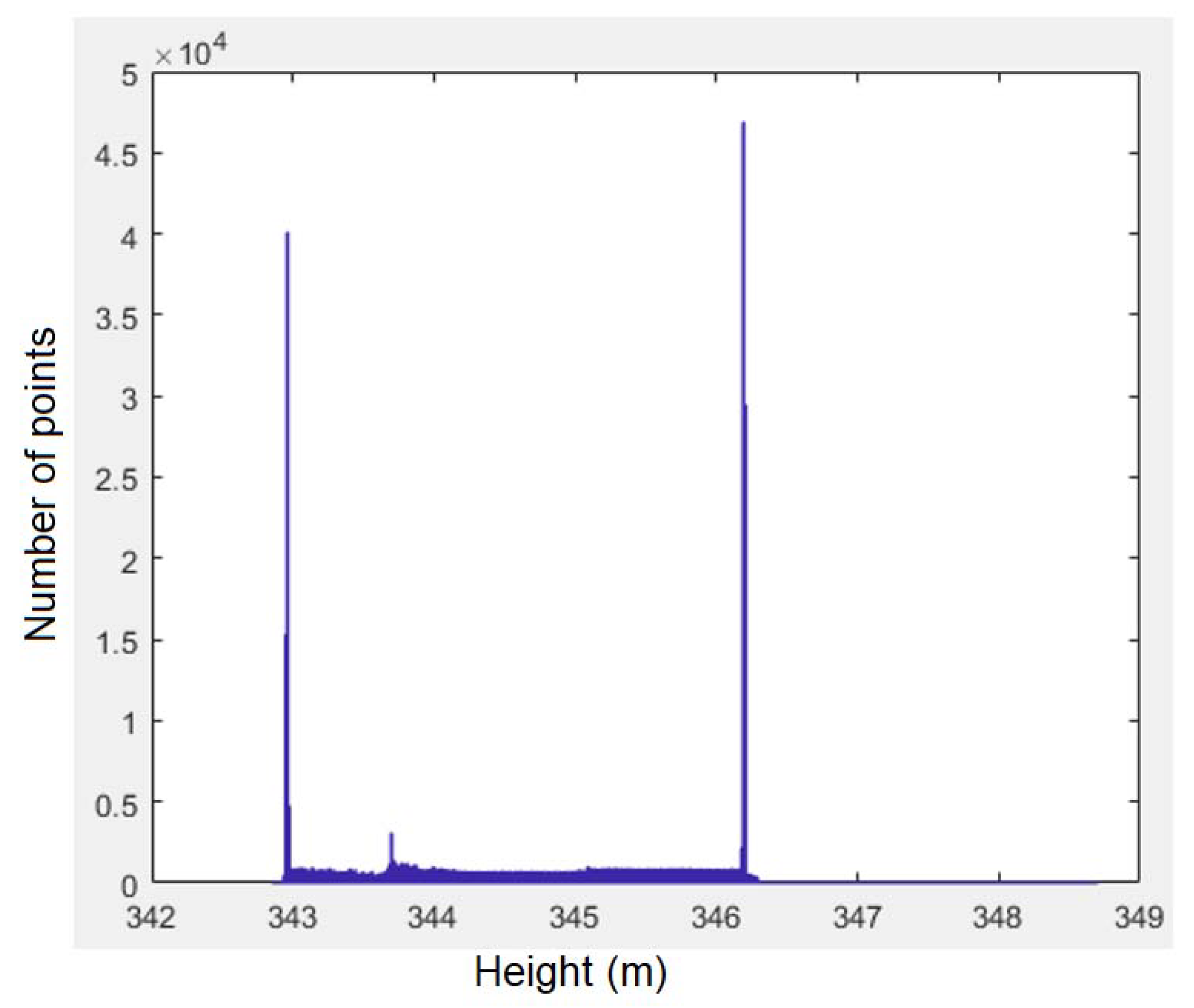
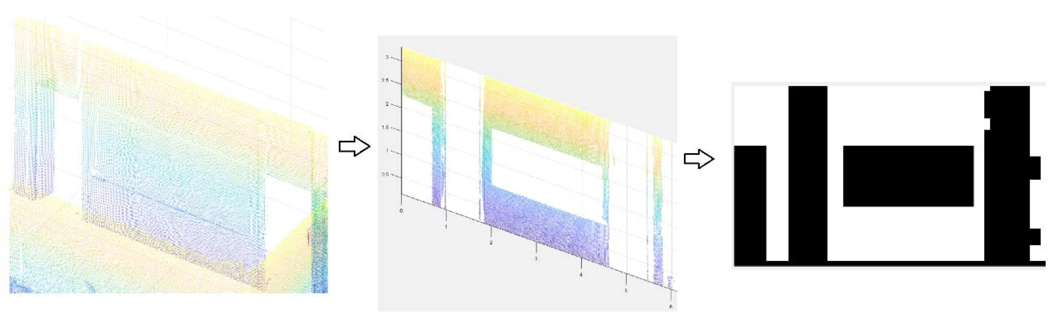
2.1. Data Collection and Pre-processing

In this work, input data consists of point clouds obtained from a laser scanner (LS) mounted on a simulated robotic system. A Faro Focus 3D X330 laser scanner was used. It is a phase-shift device with a range from 0.6 to 330 m and a field of view of 300° × 360°. Around 6 million points were collected per scan with the selected configuration of the LS that were subsampled using a point distance filter, in order to reduce computational time during processing.

In previous simulations, the LS was mounted and levelled on a robotic system; however, the resultant point cloud of the floor typically was not perfectly horizontal and the normal vector of the floor should align to the z-axis. As a first step, we obtained the normal vector of the floor plane, $n_{floor}=\left(n{f}_x, n{f}_y, n{f}_z\right)$ and its angles with the xz-plane, α and the yz-plane, β (Equation (1)):

$$\begin{array}{c}\alpha =\mathrm{atan}\left(\frac{n{f}_x}{n{f}_z}\right)\\ \beta =\mathrm{atan}\left(\frac{n{f}_y}{n{f}_z}\right)\end{array}$$

(1)

Afterward, the point cloud was levelled by applying the rotations with calculated α and β angles according to Equation (2):

$$\begin{array}{c}Rot\left(x,\beta \right)=\left(\begin{array}{ccc}1& 0& 0\\ 0& \cos \left(\beta \right)& -sin\left(\beta \right)\\ 0& sin\left(\beta \right)& \cos \left(\beta \right)\end{array}\right)\\ Rot\left(y,\alpha \right)=\left(\begin{array}{ccc}\cos \left(\alpha \right)& 0& sin\left(\alpha \right)\\ 0& 1& 0\\ -sin\left(\alpha \right)& 0& \cos \left(\alpha \right)\end{array}\right)\end{array}$$

(2)

Following that and in order to filter the point clouds corresponding to the floor and the ceiling, a rough segmentation of the point cloud was performed by considering the histogram of the z-coordinates, as is done in Adán et al. [15]. The two maximum values of the histogram correspond to the elevation of ceiling and floor (Figure 2). Segmentation of ceiling and floor points was achieved by applying a threshold assuring that 95% of the points belonging to them are filtered. The aim of this pre-processing step was to deal with the most common case, so particular examples with several floors or ceilings could be solved by considering more segmentation steps in the methodology.

Given that the LS makes use of an internal barometer to collect absolute elevations, a rigid body translation was applied to the z-coordinate of the resulting point cloud in order to reference the height of the points to the floor elevation, therefore making that the floor plane coincident with the xy plane.

In the final step of pre-processing, voxelization of the point cloud was performed in order to simplify the spatial information of the room. This voxelization resulted in a discrete space that was expected to grow to the extent that new point clouds were collected and registered to the initial acquisition. The voxel structure is stored throughout the process in the on-board computer and can be used later in other processes.

Choosing a good voxel size, l, is important and implies a trade-off between the computational cost of the classification and the loss of detail in the point cloud. In our case, we defined the voxel size taking into account the minimum size that would ensure the expected geometric results.

All the information of the voxelized space was stored in a matrix that we denote Mv(t). Each cell of Mv(t) represents a voxel. Six labels were defined to classify the voxels:

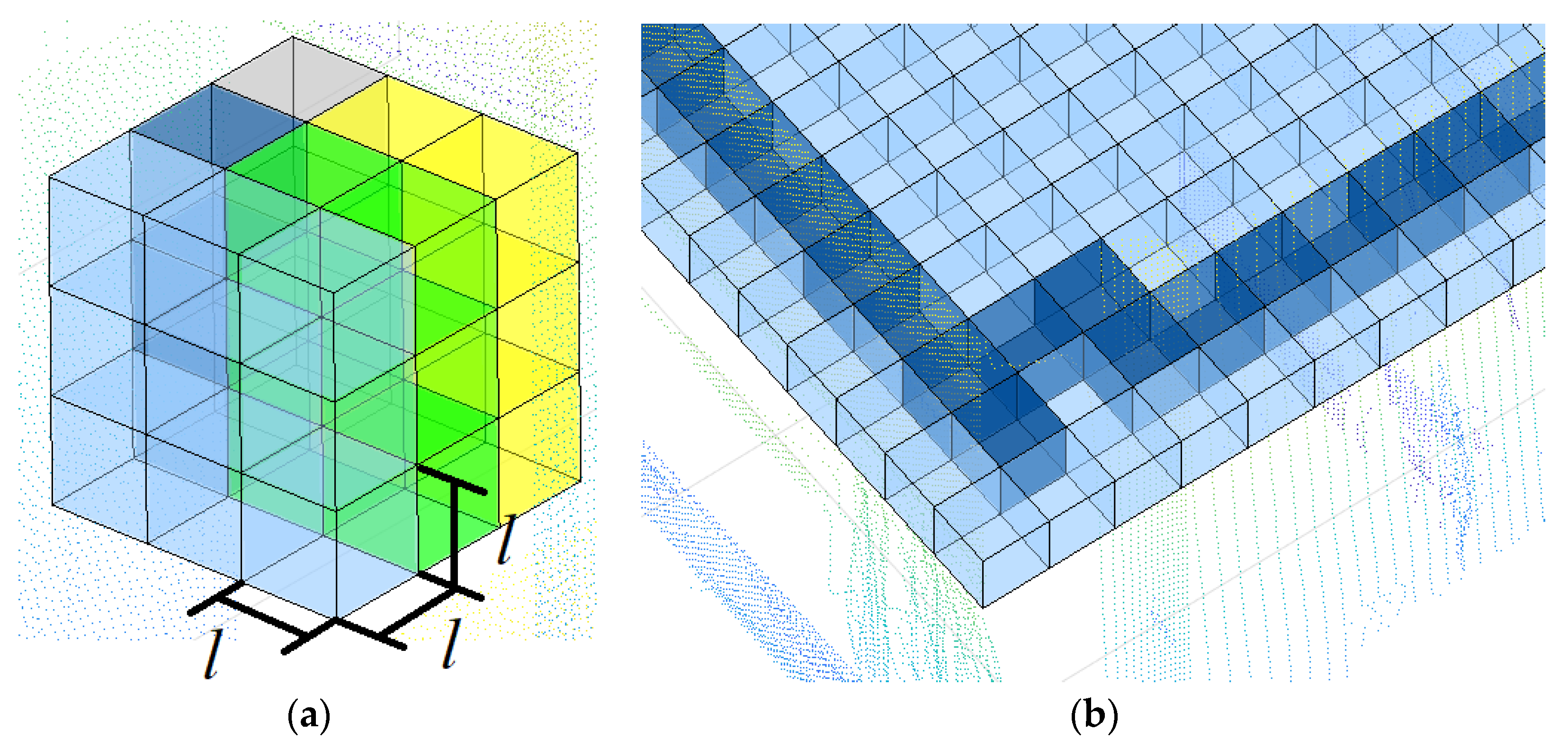
• Empty: Voxels with a direct line of sight (LOS) from the scanner position and no points inside.
• Occupied: Voxels containing a minimum number of points.
• Occluded: Empty voxels without a direct LOS from the scanner position and no points inside; their emptiness is not assured.
• NBV: (next best view) A unique empty voxel that is the optimum next scanning position.
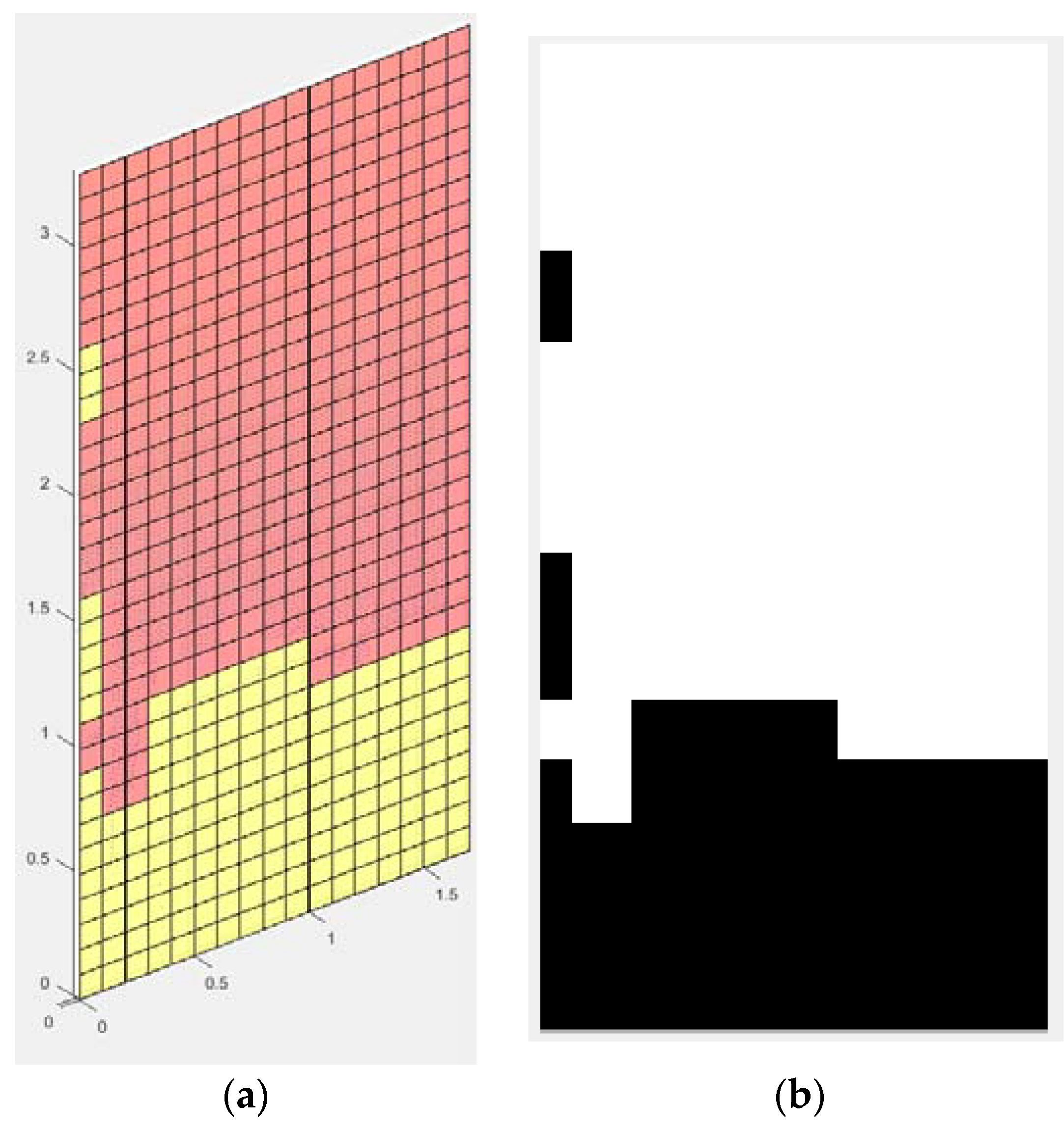
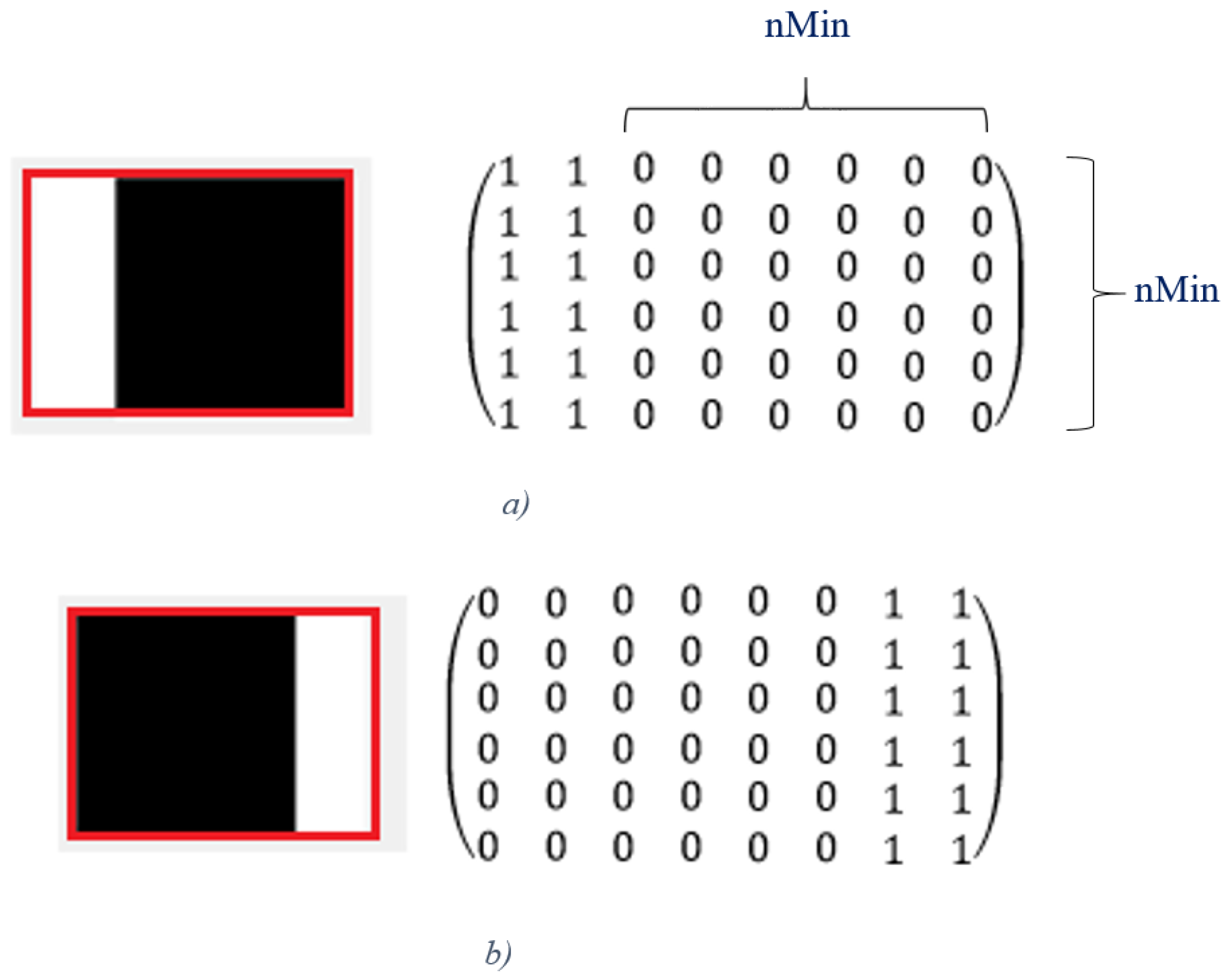
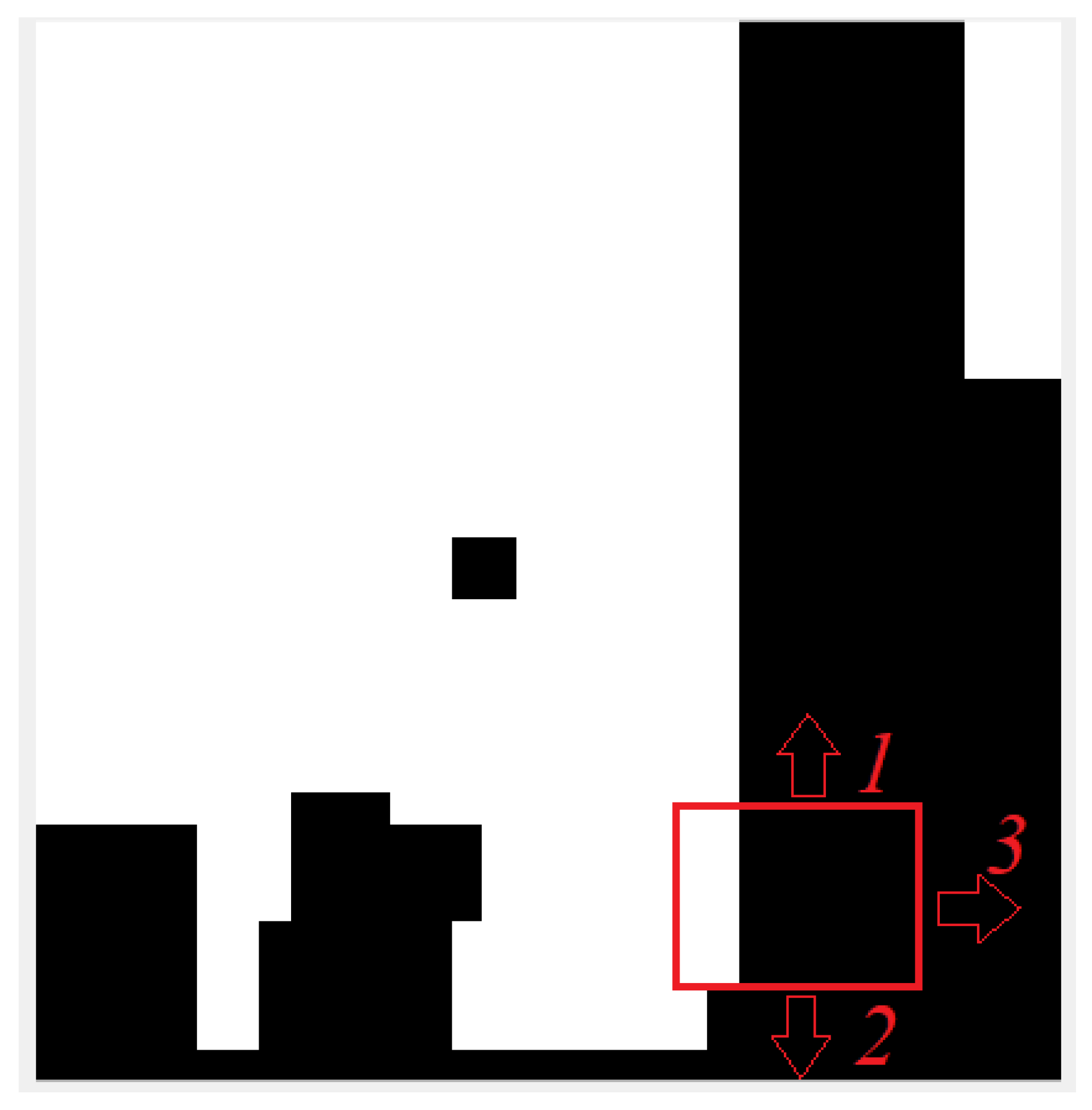
• Window: Empty voxels that belong to a window in the room.
• Door: Empty voxels that belong to a door in the room.
• Out: Empty voxels with a direct LOS from the scanner position and through a window or door voxel.

Considering that the floor plane was parallel to the xy-plane, a rotation around the z-axis was performed in order to alienate the faces of the voxels with the wall and thus optimize the voxelization of the point cloud to reduce the final number of voxels. We took into consideration that in most buildings, walls are perpendicular and parallel to each other. Accordingly, we aligned the longest wall with the xz-plane. In order to obtain the angle between the longest wall and the y-axis, segmentation of a horizontal section of the point cloud was performed at a certain distance below the ceiling. The upper part of the walls located near the ceiling are the least occluded area in most nonindustrial buildings. Afterward, the normal vector of the longest wall $n_W=\left(n{w}_x,n{w}_y,n{w}_z\right)$ was calculated and the angle $\gamma$ with respect to the y-axis derived (Equation (3)). Finally, a $\gamma$ rotation around the z-axis was applied to the point cloud (Equation (4)).

$$\gamma =\mathrm{atan}\left(\frac{n{w}_x}{n{w}_y}\right)$$

(3)

$$Rot\left(z,\gamma \right)=\left(\begin{array}{ccc}\cos \left(\gamma \right)& -\sin \left(\gamma \right)& 0\\ \sin \left(\gamma \right)& \cos \left(\gamma \right)& 0\\ 0& 0& 1\end{array}\right)$$

(4)

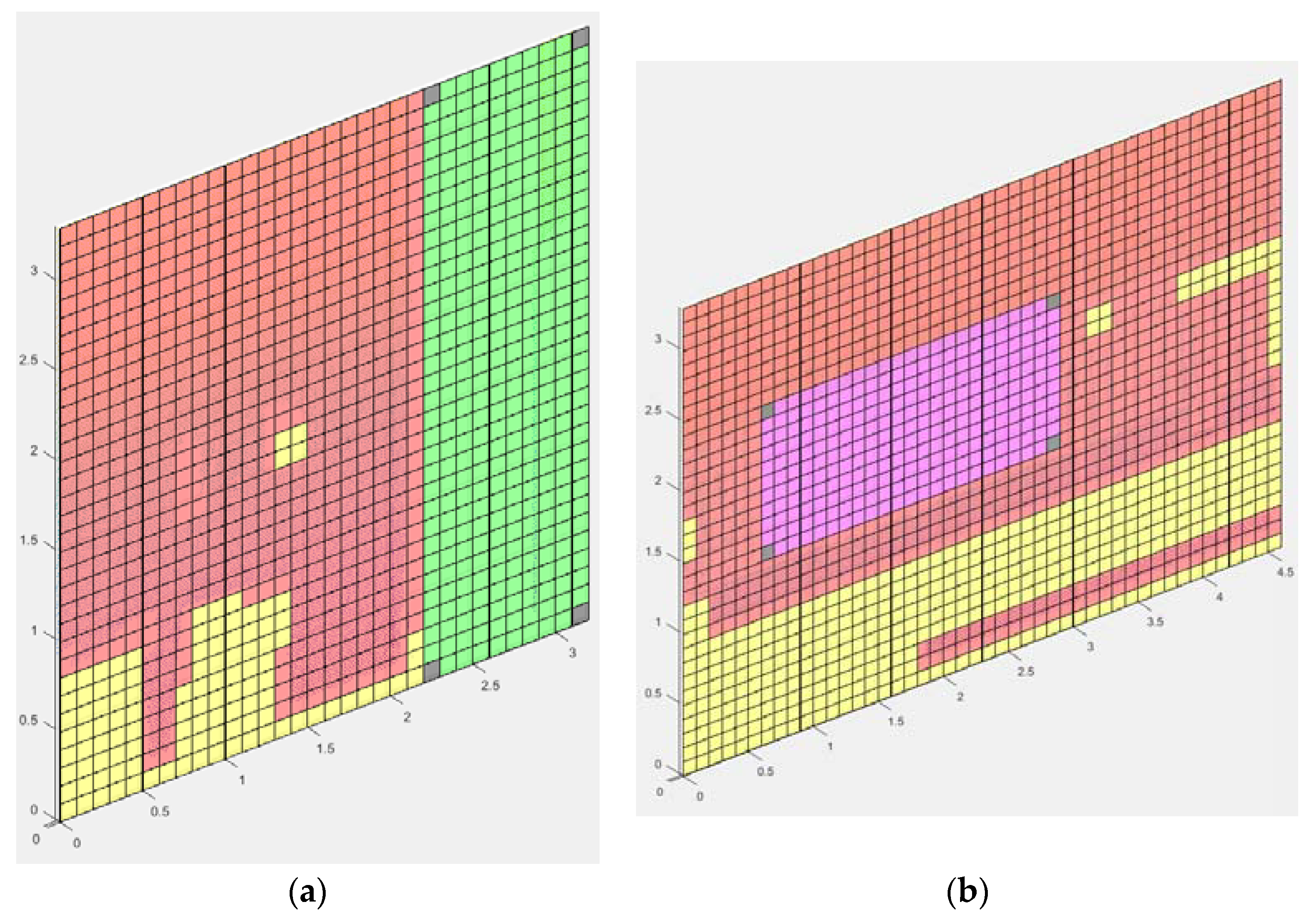
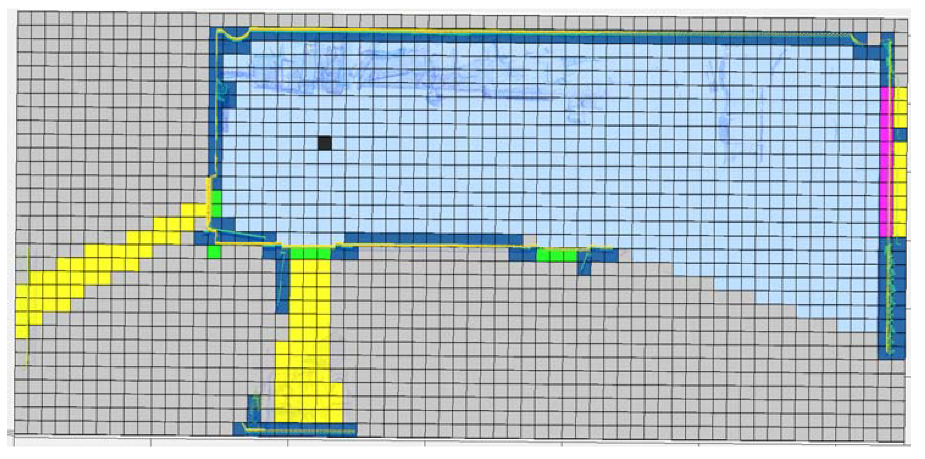
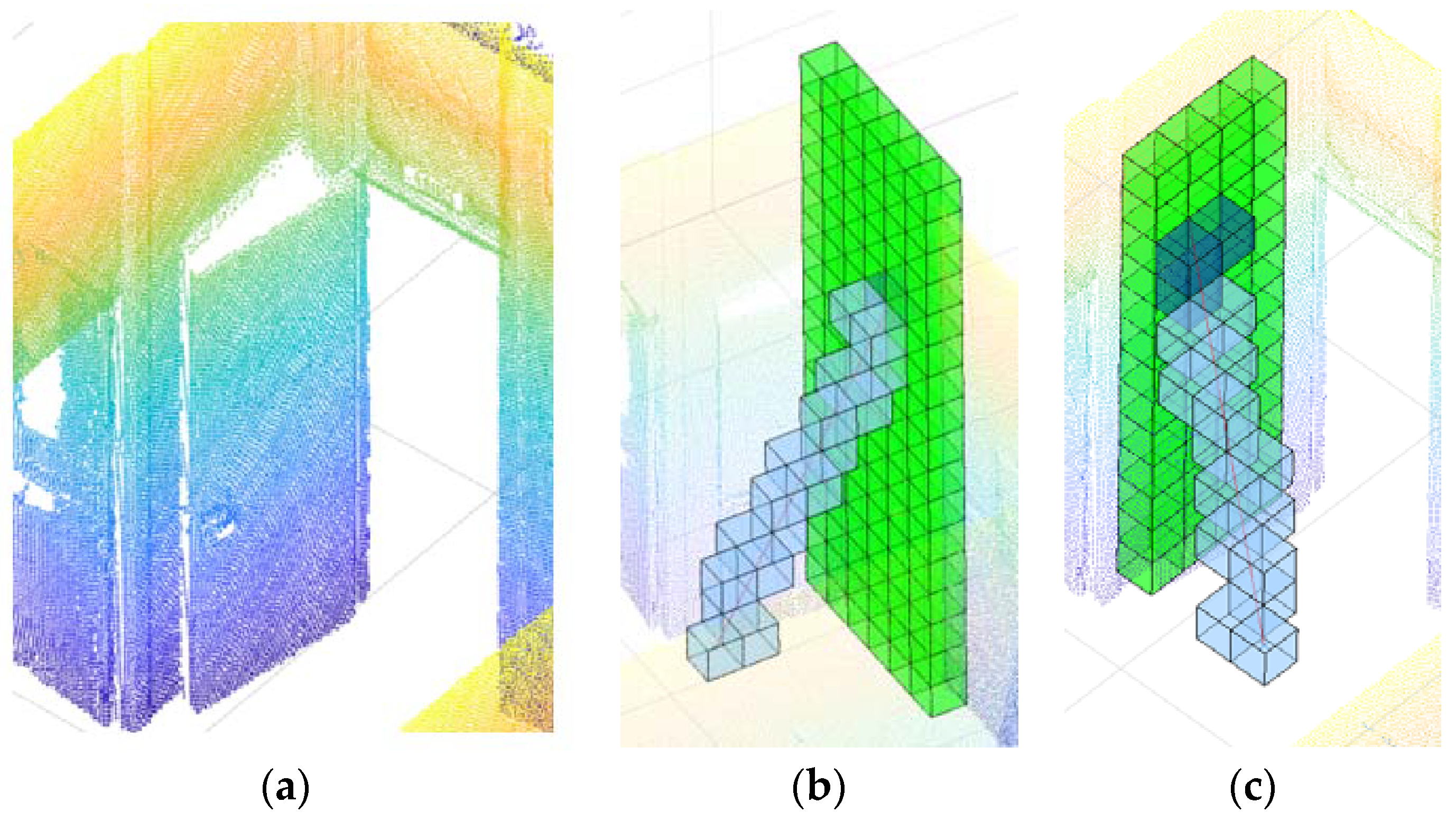
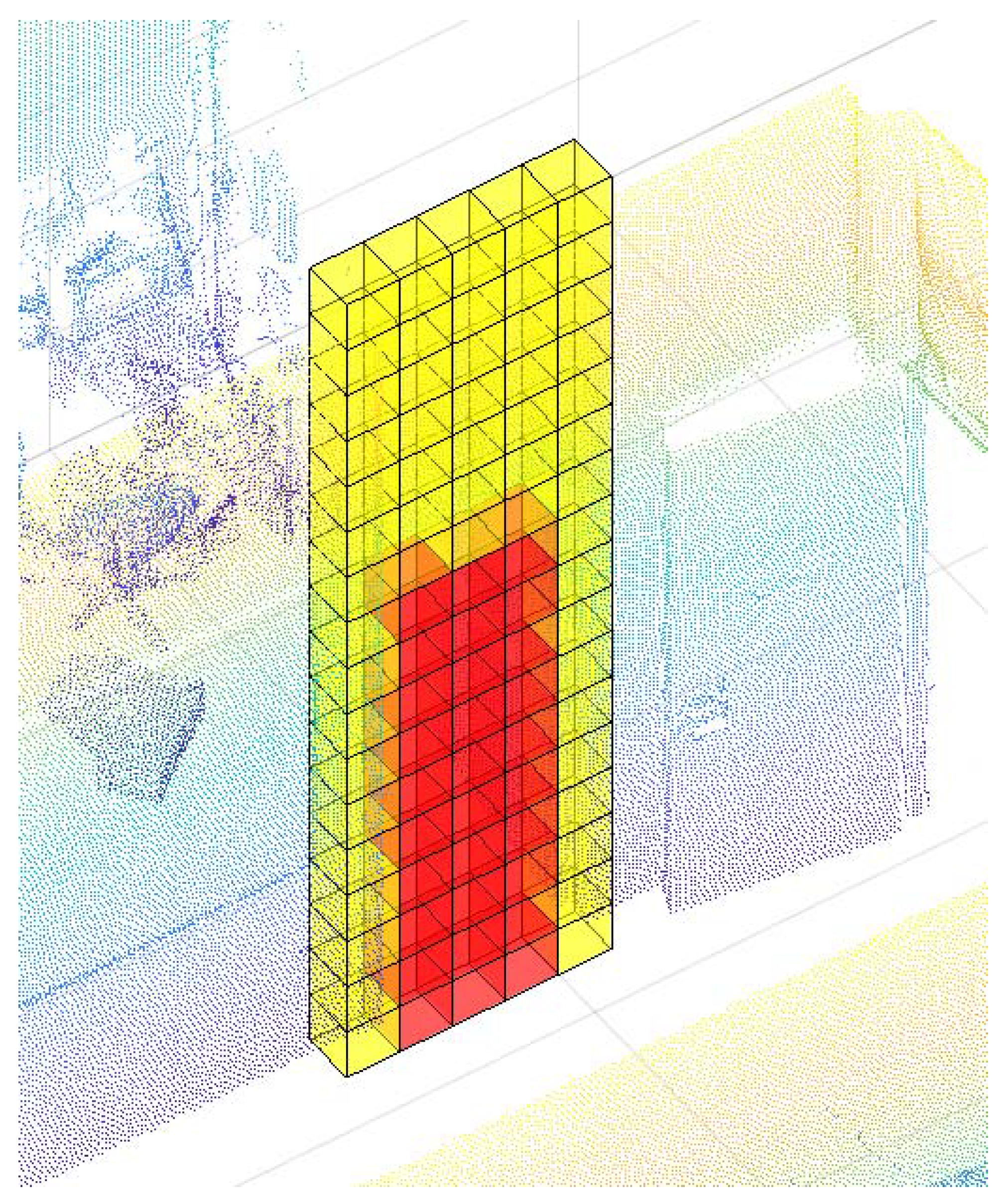
2.2. Voxel Classification

This section deals with classification of the voxels (Figure 3a), which are labelled in two steps. The first step is focused on classification of occupied and empty voxels. The second step is a refinement of the classification. It is focused on the locations of doors and windows. Classification of occluded and exterior voxels is also done in the last step.

In the first classification, differentiation between occupied and empty voxels (Figure 3b) was based on the voxel point density (i.e., the number of points in the volume of the voxel). A threshold estimating the minimum number of points to classify a voxel as occupied was established based on voxel size and empirical data. The density of voxels is of great importance, because it helps to discriminate noisy voxels or reflections that otherwise would affect the classification computations.

After the initial voxel segmentation, the methodology focuses on the locations of doors and windows and on the classification of occluded and exterior voxels.

To locate the doors and windows of the room, each segmented wall in the point cloud, P(t), needs to be analysed. The normal vector of each wall was calculated taking into consideration the horizontal section of the point cloud at a certain distance below the ceiling and based on a random sample consensus (RANSAC) algorithm [32]. As a result, the dominant plane of each wall and its points were obtained.

Once the wall planes were segmented, a binary image showing the occupancy of the plane was derived. In order to obtain the binary image, a 2D grid was computed to discretize the point cloud of the walls (Figure 4a). The grid size was chosen to match the detected doors and windows in the previous 3D voxelization.

Following that, the binary image was computed as a threshold of the 2D grid: rectangles that contained more points than the threshold corresponded to occupied pixels and those that did not fit the condition corresponded to empty pixels. All this information was stored in an image matrix, I(t), with 1-value pixels for the occupied and 0-value pixels for the empty rectangles (Figure 4b).

To locate doors and windows of the room, we used a model-driven approach: a number of patterns was designed and detected in the image. These patterns are shown in Figure 5. The design of the patterns was based on the minimum size of the detectable hole, nMin and was a trade-off between the number of false positives (smaller values of the filter) and the likelihood of detection (longer values of the filter). The filtering process consisted of applying a morphological opening and closing to the image I(t) [33] using the designed models as structuring elements s (Equation (5)). As a result, two main objectives were achieved: edge homogeneity improved and small isolated areas were filtered out of the image I(t) (Figure 6).

$$s=\left(\begin{array}{ccc}1& 1& 1\\ 1& 0& 1\\ 1& 1& 1\end{array}\right)$$

(5)

A sliding window filter was applied to the image, looking for the pattern in the image and extended up and down and to the sides when found (Figure 7), rejecting false positives that resulted from occlusions that matched the pattern but had irregular shapes. The rejection of these false positives was based on the variance of the recognized pattern: irregular results with high variance were marked as false positive and discarded (Figure 8). The recognized patterns that passed the previous tests were classified as “door” if the pattern reached the floor, or as “window” otherwise.

In order to obtain a “door/window” assessment, we carried out a visibility study that consisted of checking whether the hole was due to an occlusion or not. For example, that would be the case if a blackboard caused a window-shaped hole (Figure 9) or a locker near the wall generated an occlusion with a door shape (Figure 10a). This assessment consisted of comparing the recognized patterns on the wall with the previous 3D voxel classification based on a ray-tracing study from the scanner position (Figure 10b).

In case we found a direct LOS from the voxels to the LS position, a window/door hole was confirmed and the classification of the voxel was updated from “empty” to “door/window.” On the contrary, when a significant number (>85%) of voxels inside a hole did not have a direct LOS from the LS position, their classification was left without changes (Figure 10c). Moreover, if we did not have direct LOS from the LS to all the pixels in a window/door candidate, it would not mean that the detected element was a false positive. For example, it is possible that some object, such as a chair or piece of furniture, could occlude part of the detected hole; so, if we had direct LOS for 15% of the candidate voxels, the voxel classification was updated to mark a window/door. The occluded voxels that were misclassified as window/door was an issue for the following steps of the methodology. Finally, we took into consideration that there might be occupied voxels that were part of the recognized pattern (Figure 11) and gave priority to their previous classification. This means that if a candidate window/door voxel was labelled as occupied, it always maintained such classification.

At this point, we classified four types of voxels: occupied, empty, door and window. Three of these classes remained unchanged but we submitted the empty voxels to a second ray-tracing in order to classify the occluded and outer voxels. To recall, occluded voxels are empty voxels without a direct LOS from the scanner position (Figure 12a), while outer voxels are empty voxels with a direct LOS from the scanner position through a window/door voxel (Figure 12b).

We defined voxels with a direct LOS as those for which the ray traced between their centres and the scanner position did not cross any occupied voxel. In other words, the ray only went through empty voxels. If an empty voxel did not have a direct LOS, that meant the laser scanner was not able to reach that area because of some kind of occlusion and therefore it was classified as an occluded voxel. On the other hand, if a voxel showed direct LOS and crossed any voxel labelled as “window/door,” it was considered an outer voxel and classified as “out.”

We followed this ray-tracing-based classification for all the empty voxels left, until the discretization of the room was completed (Figure 13).

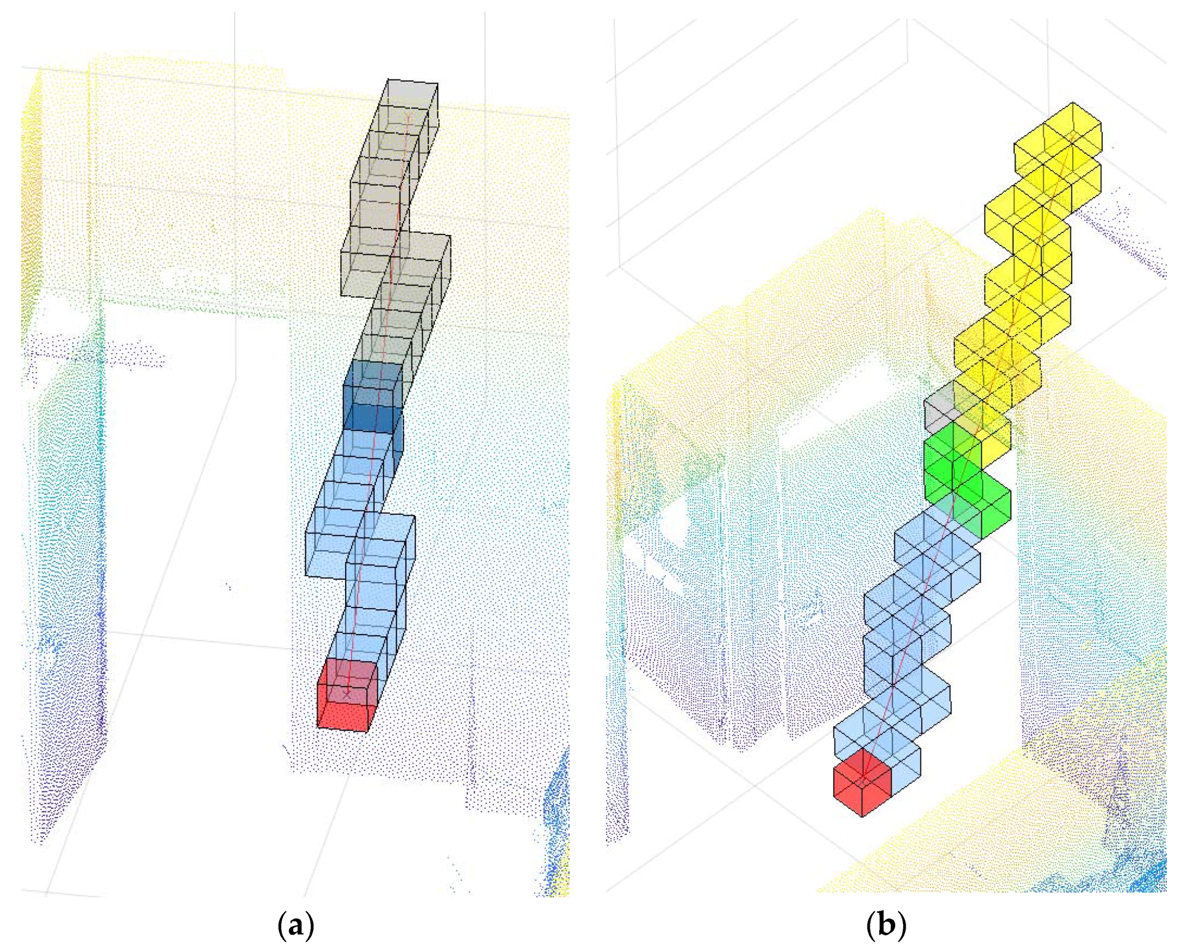
2.3. Next Best View

The main objective of this method was to calculate the optimum scanning position to automatically perform complete scanning of the site with the minimum number of scans, starting from an arbitrary position in the room and without any other previous information. This optimal scanning position was defined as next best view (NBV). This is the position where the robot should stop to perform the scan using a stop-and-go survey procedure.

To calculate the NBV, the previously created voxel space was used (Figure 13). The method consisted of checking the feasibility of every voxel as an NBV candidate in terms of safety and significance.

The safety condition takes into account the size of the scanner station ($h_{scanner}$ = 1.5 m). It is defined as a cylinder-centred buffer on the candidate voxel with height $h_{scanner}+0.5 \mathrm{m}$ and a security radius $r_s$ that is defined. All the voxels contained in this cylinder must be empty voxels as an assessment that the LS is in a safe position during the scanning process.

Additionally, to assess the significance of an NBV candidate, a scoring system was defined. A ray-tracing study was conducted, selecting the NBV candidate as the origin of the beam and checking the number of occluded voxels with direct LOS from the candidate. The NBV was the voxel that got the highest score.

For this purpose, a semi-direct LOS was defined as the line-of-sight ray between two voxels that crossed not only empty but occluded voxels but never occupied voxels. In this case, a direct LOS for this voxel could not be assured.

In order to give importance to the broad areas occluded in the room, we introduced a new variable, $n_{OV}$, which is the maximum number of occluded voxels that we allow to cross the line of the semi-direct LOS to continue scoring in the calculation of NBV. The intention was to give more importance to areas that are likely to be an extended occluded zone of the site. A trade-off was necessary, because if the value of this variable were too small, it would hardly have an effect on the NBV calculation and such occluded zones would not be considered. On the other hand, if the variable were too large, it would cause the NBV to focus only on eliminating the occlusions in such zones.

Each NBV candidate started with a score $S_{nCandidate}$ equal to zero and increased with $S_i$ score values obtained from the ray-tracing step and for each occluded voxel (Equation (6)). The following scores $S_i$ for each occluded voxel were considered:

• Zero-point score if there was not a direct LOS between the NBV candidate and the objective occluded voxel.
• One-point score if there was a direct LOS between the NBV candidate and the objective occluded voxel.
• In case of a semi-direct LOS from the NBV candidate, the score $S_i$ was calculated according to Equation (7), where $n_{CrossedOV}$ is the number of intermediate occluded voxels crossed.

  $$S_{nCandidate}={\displaystyle \sum }_{i=1}^{nOccludedVoxels}{S}_i$$

  (6)

  $$S_i=\frac{1}{1+n_{CrossedOV}}$$

  (7)

If more than one candidate obtained the maximum score, the candidate closest to the current scanner position would be chosen as NBV. In addition, we added a stopping criterion for the scanning process in order to determine when the entire site was documented. This stopping criterion consisted of calculating the percentage of occluded voxels $n_{Voccluded}$ with a direct or semidirect LOS from the NBV with respect to the total number of unoccluded voxels (i.e., empty, $n_{Vempty}$, occupied, $n_{Voccupied},$ and outer, $n_{Vout}$, voxels) of the site (Equation (8)):

$$StopPercentage=\left(\frac{n_{Voccluded}}{n_{Voccluded}+n_{Vempty}+n_{Voccupied}+n_{Vout}}\right)\times 100$$

(8)

when this StopPercentage was lower than a defined threshold, the whole site was already scanned. The voxels classified as doors might be selected as the next site for scanning.

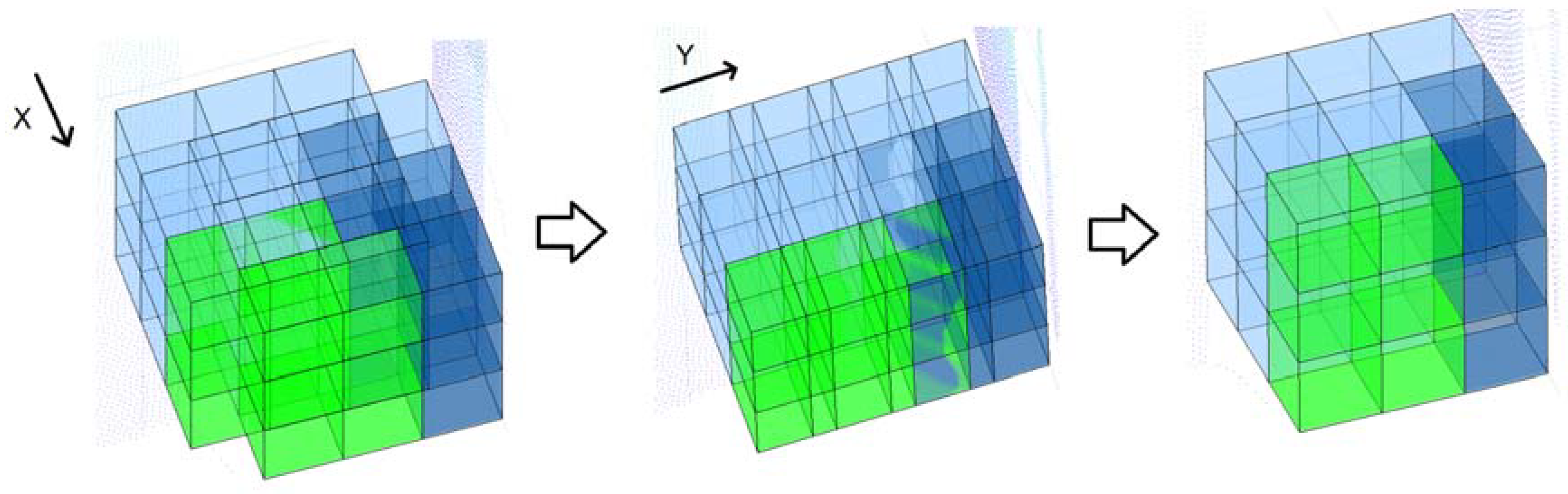
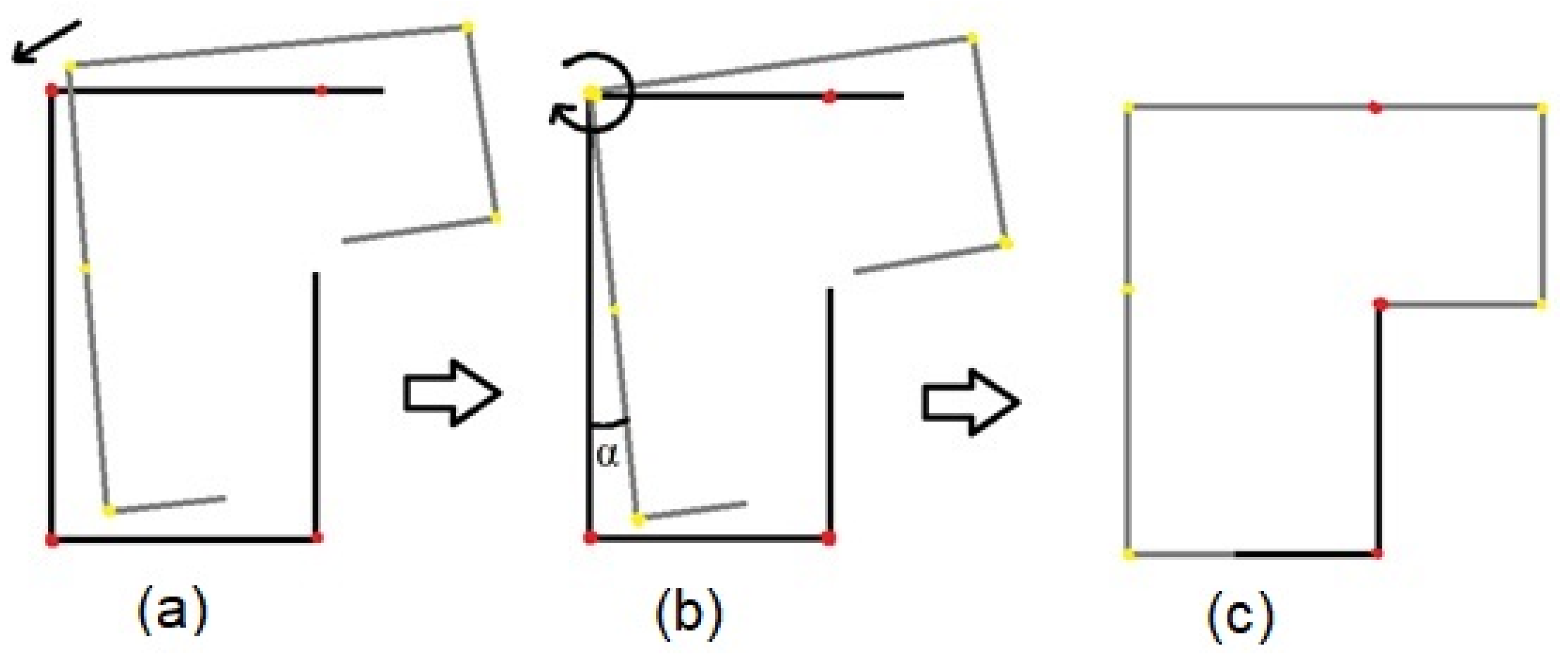
2.4. Scan Registration and Voxel Growing

Once the robotic system was moved to the NBV and performed the next scan, the current point cloud P(t) and the previous point cloud P(t − 1) were registered. Taking into account the theoretical position of the robotic system at the NBV, a coarse registration was done, followed by a fine registration. This registration process exploited the pre-processing step described in Section 2.1. The plane of the floor was horizontal at zero height and coincident with the xy plane, so this registration consisted of an xy-translation and a z-rotation.

For the coarse registration, the rotation angle and the translation were calculated as follows. The angle of rotation was calculated according to the navigation data of the robotic system, adding the rotation that we applied to the former point cloud in the voxelization step. The translation was calculated by subtracting the position of the NBV from the position of the previous scan. This coarse procedure did not fit the requirements of an optimum registration, because the robotic system would not be exactly in the NBV position and because of measurement errors. A fine registration of both point clouds was performed, taking into consideration the geometry of the site, following the next steps.

First, the intersection points between each pair of nonparallel wall planes and a horizontal plane were calculated (Figure 14a). Again, a section of the point cloud at a certain height was used to calculate the planes of the walls, all the intersection points between those planes and a horizontal plane were obtained for both point clouds and the distance between the points in the new and previous point clouds was derived.

Considering these calculated distances, the closest points between both point clouds were selected and the new point cloud was translated in order to make both points coincide (Figure 14b). The new distances between intersection points (excluding the pivoting point) of both point clouds were calculated again and the nearest points were selected. These two pairs of points were used to calculate the α angle between point clouds and after z-axis rotation, the current point cloud was accurately registered to the former point cloud (Figure 14c).

Once both point clouds were registered, voxelization of the entire point cloud was performed, taking into account that both the previous and new voxelizations must coincide in order to transfer the former voxel classification to the new voxelization. To make both point clouds coincide, an xy-translation was applied on the total point cloud (Figure 15).

Once both voxelizations were coincident, we compared the classification values of the new voxelization with the previous voxelization considering that the attributes of the occluded voxels might have changed while the other classes had to remain unchanged. Therefore, occluded voxels of the new voxelization inherited the previous classification.

3. Results and Discussion

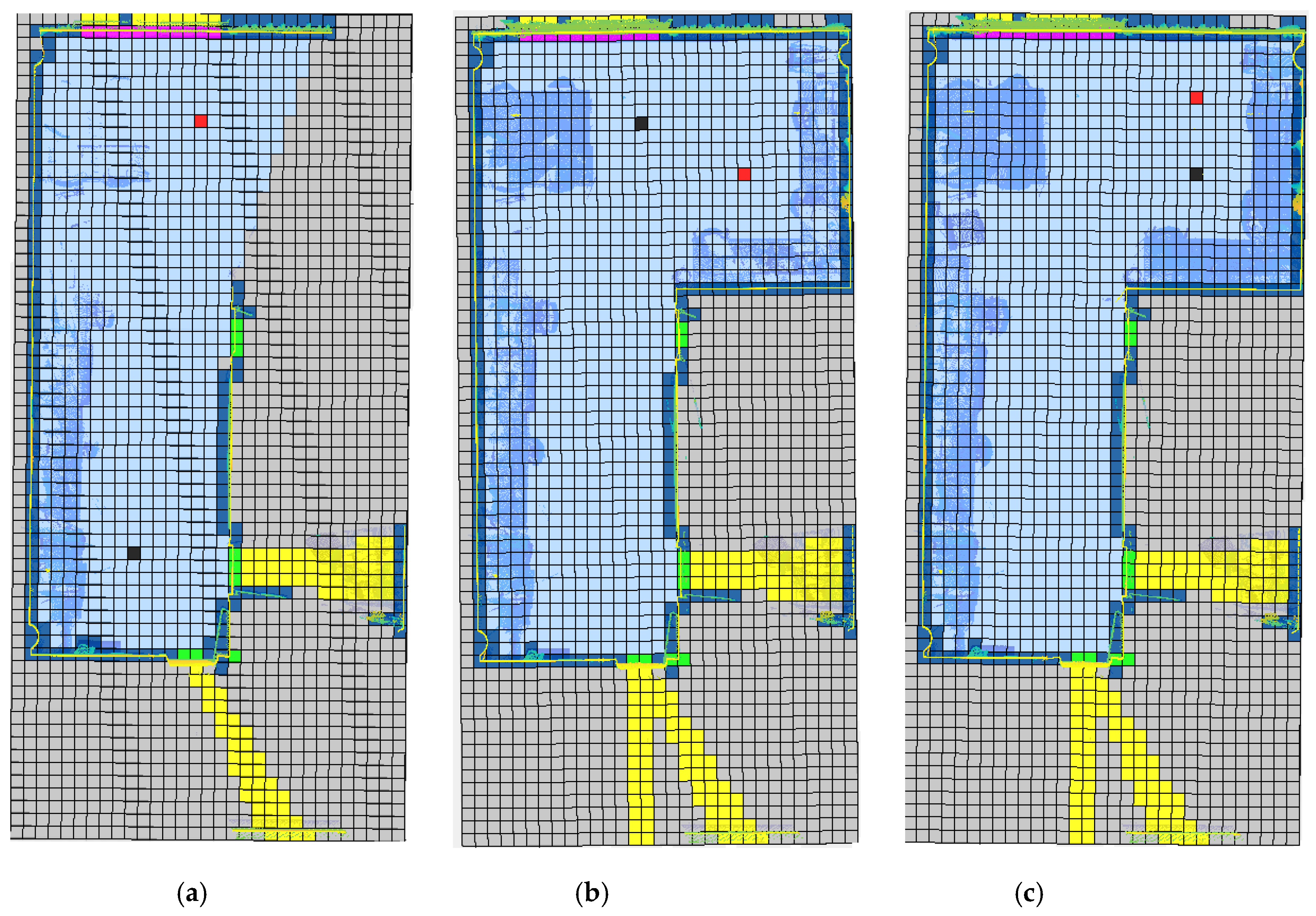
Case Study

This study was carried out in a laboratory of the Mining and Energy Engineering School at the University of Vigo. This laboratory has three doors and a large window with a semi-open curtain (Figure 16). The size of the study room was approximately 10 m × 6 m, with a stop percentage of 0.1%. A total of three scans were taken, which supposed approximately 1.4 million points of the pre-processed point cloud with the distance filter (20.4 million points without filtering). The voxelization of the discretized study room contains 34,255 voxels of 20 cm size. Pre-processing of the three point clouds, voxelization and calculation of the NBV took 1 m, 45 s using an Intel core i7 and 16 Gb of RAM. If we add in the scanning time, which in our case with the selected scanning parameters was 1 min, 30 s per scan, the total time for scanning the room was 6 min, 15 s. This does not take into account the travel time of the robotic system.

In Figure 17 we can see the value of the voxels in the horizontal plane in which the scanner moved for each scan. In Figure 18 we can see a 3D visualization of how the classification of the occluded voxels of the interior of the room changed in each scan.

All the algorithms for point cloud processing were implemented in MATLAB 2017b, using the Point Cloud Library. As mentioned before, the scanning process was carried out with a Faro Focus 3D X330 LiDAR scanner. Each point cloud had about 3.8 million points, which, after applying the filtering, remained at about 480,000 points. In

Table 1. Percentage of voxels of each type and total number for each scan.

Scan Number	V. Occluded	V. Occupied	V. Empty	V. Door	V. Window	V. Out	Total Voxels	V. Matrix Dimension
First Scan	55.69%	7.03%	34.16%	0.31%	0.14%	2.67%	34,255	65 × 32 × 17
Second Scan	43.49%	10.54%	42.14%	0.27%	0.13%	3.44%	34,255	65 × 32 × 17
Third Scan	42.35%	11.76%	42.15%	0.27%	0.13%	3.34%	34,255	65 × 32 × 17

we can see the percentage of voxels of each type, the total number of voxels and the dimensions of the voxelization matrix for each of the three point clouds. So, we can see how the number of occluded voxels decreased with each new scanning, while the number of empty and occupied voxels grew. It is very important to correctly select the threshold of number of points that a voxel must contain in order to be classified as occupied. This parameter depends on the previous filtering applied and the selected voxel size. For our case, we empirically verified that the value that best represented the reality was 20 points/occupied voxels for the selected voxel size (

Table 2. Number of occupied voxels in each scan for different numbers of points within an occupied voxel.

Scan Number	5 Points	10 Points	20 Points	30 Points	40 Points
First Scan	2782	2646	2408	2164	1946
Second Scan	4061	4060	3610	3394	3171
Third Scan	4319	4321	4030	3678	3483

).

For the selection of voxel size, we must bear in mind that a large voxel size, like 1 m, will not represent reality but will have a very fast processing, while a small voxel size, like 5 cm, will have good resolution but very slow processing. Therefore, we must have a voxel size that assures the wanted scan results. In this case, we focused on the geometric requirements to select the voxel size. For our case, we scanned not only the structural components of the room but also the furniture (i.e., tables, chairs). Also, for our robotic system to move safely, we chose a security radius of 0.6 m, because it needed a safety cylinder 1.2 m in diameter. Therefore, we chose a voxel size of 20 cm, which is the third part of the most critical measurement that we should capture and less than the half part of the standard sizes of tables and chairs.

We must bear in mind that there are occluded voxels outside the room, so we will never have direct or semi-direct vision of them from the NBV. In

Table 3. Number of occluded voxels with direct or semi-direct line of sight (LOS) from the NBV and stop percentage calculated.

Scan Number	nV Occluded	Stop Percentage
First Scan	549	3.5%
Second Scan	65	0.35%
Third Scan	18	0.09%

, we can see the number of occluded voxels of which we have direct or semi-direct vision from the NBV and stop percentage calculated for each scan.

In the pre-processing of the point cloud, we used a distance threshold for segmentation of the ceiling and floor. The chosen value of this threshold was 5 cm. This value was chosen because we adjusted the peaks of the z-histogram to a Gaussian distribution, where the value of the deviation σ was calculated as 2.5 cm. Therefore, we use 2σ as the threshold to be sure that 95% of the points belonging to the floor and ceiling were within the point cloud we segmented.

We aligned the longest wall of the first scan with the x-axis to optimize the voxelization. If we did not align this wall, we would have 51,646 voxels in a matrix of 62 × 49 × 17, compared to 34,255 voxels in a matrix of 56 × 32 × 17 if we aligned the wall (50.5% more voxels). This amount depends on the initial angle of the first point cloud. If the voxelization is not optimized, the method will work exactly the same but will be slower, because the voxelization matrix will be greater.

When we were detecting the doors and windows of the room in the fine classification, we had to define the dimensions of the search pattern. As we explained in Section 2.2, we used half the voxel size for the rectangle size in the discretization of walls, so the side size l of the rectangles was 10 cm. As we had to detect doors and the minimum standard size of doors is 70 cm, we used 50 cm as the size of the pattern. This dimension provided a margin of 20 cm to absorb the possible errors due to irregularities in the point cloud.

The value of the minimum threshold of variance to distinguish between door- and window-shaped holes on the wall and false positives was derived empirically. A case study was made and the variance was calculated for each pattern of doors and windows to be able to limit them with a threshold (Figure 19). As expected, the variance calculated for each door/window was low (

Table 4. Variance and area calculated for each pattern detected.

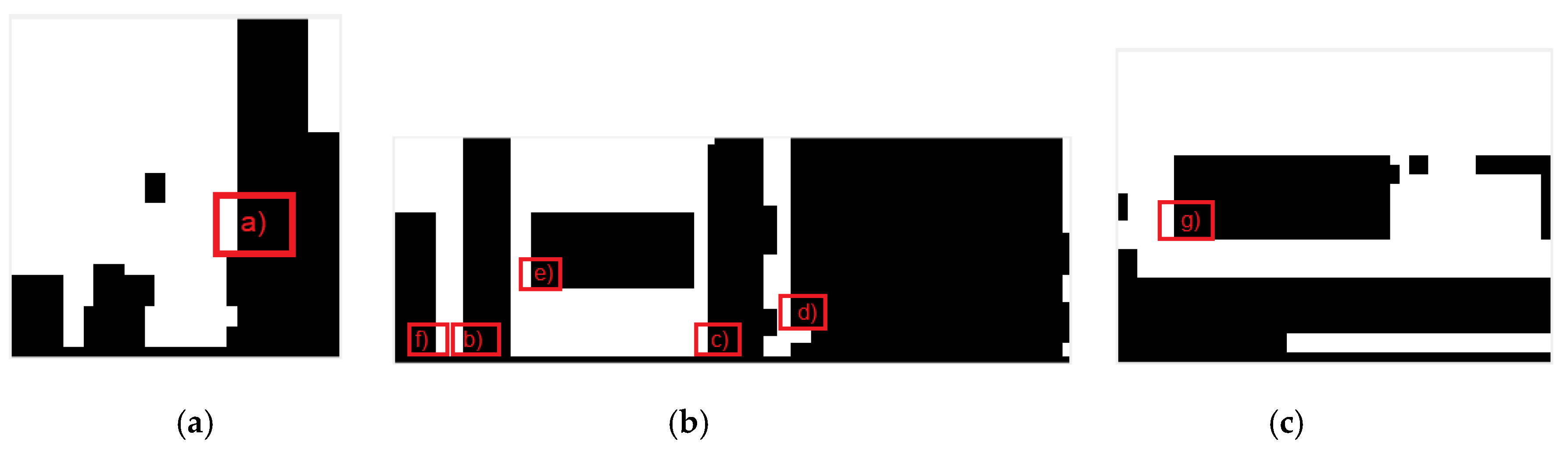
Pattern	var(nRowsBelow)	var(nRowsAbove)	var(nColumns)	Area (m2)	Door/Window
(a)	0	0	2.0625	3.3	True
(b)	0	0	0	2.31	True
(c)	0.1429	0	3.1894	2.64	True
(d)	0	7.14	6.2476	13.2	False
(e)	0	0	0	2.64	True
(f)	0	0	0	1.32	True
(g)	0	0	0.1944	2.07	True

), since we were looking for a well-defined rectangular pattern. The value used for this threshold was 10. Also, we have a maximum area value for a door/window, which for our case we define as $5 {\mathrm{m}}^2$. This way of detecting doors and windows will not be valid, for example, for detecting windows that occupy a whole wall or windows that do not have straight sides.

A good registration between two consecutive point clouds is very important to be able to pass all the information from the voxelization of one scan to another. With the registration method used, very good results were obtained, as can be seen in Figure 20, in which the distance between the closest points between consecutive point clouds were calculated after registration. In this figure, the blue areas represent the common areas between two point clouds, while the rest represents occluded areas or zones that only belong to one capture. As we can see in the second histogram of Figure 20, with this method of registration, the distance between the point clouds registered is approximately 1 cm, 20 times less than the voxel size used, so it is a valid method of registration for many AEC purposes.

The main weakness of this registration method is that we must have at least two common intersection points between consecutive captures. As the NBV is going to be in an area that has direct vision from the scanner position, this problem is not so important. This registration method will be effective in all rooms, where at least three walls can be seen from the two scan positions. It will not be effective if the three walls are not visible, because the method needs two intersection points between walls. In addition, for this method we can obtain more intersection points, using it for furniture such as lockers, or structural elements such as columns.

4. Conclusions

The use of 3D data from point clouds is an increasingly common practice in a wide variety of industries, so automating and optimizing the data acquisition process is fundamental.

Most of the works related to automatic scanning only include three types of voxels for space labelling, without locating the open doors and windows of the room, not giving more value to the occluded areas of the room, using an ICP algorithm for point cloud registration and without mentioning the system used for voxel growth.

The method presented here meets and improves on all these aspects, locating the doors and windows of the room, delimiting from them the study room, giving depth to the study of visibility for selection of the NBV, using the geometry of the room for the registration of point clouds and solving the growth of voxelization.

Many more things should be improved in the future, such as the design of a discretization system that allows us to improve the resolution without increasing the computational load. However, the presented method is already capable of completely automating the scanning of a room, locating the doors and windows and delimiting the room.

References

- Navon, R. Research in automated measurement of project performance indicators. Autom. Constr. 2007, 16, 176–188. [Google Scholar] [CrossRef]
- Boukamp, F.; Akinci, B. Automated processing of construction specifications to support inspection and quality control. Autom. Constr. 2007, 17, 90–106. [Google Scholar] [CrossRef]
- Akinci, B.; Boukamp, F.; Gordon, C.; Huber, D.; Lyons, C.; Park, K. A formalism for utilization of sensor systems and integrated project models for active construction quality control. Autom. Constr. 2006, 15, 124–138. [Google Scholar] [CrossRef] [Green Version]
- Bosché, F. Automated recognition of 3D CAD model objects in laser scans and calculation of as-built dimensions for dimensional compliance control in construction. Adv. Eng. Inform. 2010, 24, 107–118. [Google Scholar] [CrossRef] [Green Version]
- Xiao, Y.; Zhan, Q.; Pang, Q. 3D data acquisition by terrestrial laser scanning for protection of historical buildings. In Proceedings of the International Conference on Wireless Communications, Networking and Mobile Computing (WiCom 2007), Shanghai, China, 21–25 September 2007. [Google Scholar]
- Borrmann, D.; Hess, R.; Houshiar, H.; Eck, D.; Schilling, K.; Nüchter, A. Robotic mapping of cultural heritage sites. Int. Arch. Photogramm. Remote Sens. Spat. Inf. Sci. 2015, 40, 9. [Google Scholar] [CrossRef]
- Bosché, F.; Guenet, E. Automating surface flatness control using terrestrial laser scanning and building information models. Autom. Constr. 2014, 44, 212–226. [Google Scholar] [CrossRef]
- Díaz-Vilariño, L.; Conde, B.; Lagüela, S.; Lorenzo, H. Automatic detection and segmentation of columns in as-built buildings from point clouds. Remote Sens. 2015, 7, 15651–15667. [Google Scholar] [CrossRef]
- Bueno, M.; Díaz-Vilariño, L.; González-Jorge, H.; Martínez-Sánchez, J.; Arias, P. Quantitative Evaluation of CHT and GHT for Column Detection under Different Conditions of Data Quality. J. Comput. Civ. Eng. 2017, 31, 04017032. [Google Scholar] [CrossRef]
- Elberink, S.O.; Vosselman, G. Quality analysis on 3D building models reconstructed from airborne laser scanning data. ISPRS J. Photogramm. Remote Sens. 2011, 66, 157–165. [Google Scholar] [CrossRef]
- Soudarissanane, S.S.; Lindenbergh, R.C. Optimizing terrestrial laser scanning measurement set-up. In Proceedings of the ISPRS Workshop Laser Scanning, Calgary, AB, Canada, 29–31 August 2011; Volume XXXVIII (5/W12). [Google Scholar]
- López-Damian, E.; Etcheverry, G.; Sucar, L.E.; López-Estrada, J. Probabilistic view planner for 3D modelling indoor environments. In Proceedings of the 2009 IEEE/RSJ International Conference on Intelligent Robots and Systems (IROS), St. Louis, MO, USA, 11–15 October 2009. [Google Scholar]
- Budroni, A.; Boehm, J. Automated 3D reconstruction of interiors from point clouds. Int. J. Archit. Comput. 2010, 8, 55–73. [Google Scholar] [CrossRef]
- Previtali, M.; Scaioni, M.; Barazzetti, L.; Brumana, R. A flexible methodology for outdoor/indoor building reconstruction from occluded point clouds. ISPRS Ann. Photogramm. Remote Sens. Spat. Inf. Sci. 2014, 2, 119. [Google Scholar] [CrossRef]
- Adan, A.; Huber, D. 3D reconstruction of interior wall surfaces under occlusion and clutter. In Proceedings of the International Conference on 3D Imaging, Modeling, Processing, Visualization and Transmission (3DIMPVT), Hangzhou, China, 16–20 May 2011. [Google Scholar]
- Lee, Y.-C.; Park, S.-H. 3D map building method with mobile mapping system in indoor environments. In Proceedings of the 16th International Conference on Advanced Robotics (ICAR), Montevideo, Uruguay, 25–29 November 2013. [Google Scholar]
- Kotthauser, T.; Soorati, M.D.; Mertsching, B. Automatic reconstruction of polygonal room models from 3D point clouds. In Proceedings of the IEEE International Conference on Robotics and Biomimetics (ROBIO), Shenzhen, China, 12–14 December 2013. [Google Scholar]
- Blaer, P.S.; Allen, P.K. Data acquisition and view planning for 3-D modeling tasks. In Proceedings of the IEEE/RSJ International Conference on Intelligent Robots and Systems, San Diego, CA, USA, 29 October–2 November 2007. [Google Scholar]
- Potthast, C.; Sukhatme, G.S. A probabilistic framework for next best view estimation in a cluttered environment. J. Vis. Commun. Image Represent. 2014, 25, 148–164. [Google Scholar] [CrossRef] [Green Version]
- Xiao, J.; Owens, A.; Torralba, A. Sun3D: A database of big spaces reconstructed using Sfm and object labels. In Proceedings of the IEEE International Conference on Computer Vision (ICCV), Sydney, Australia, 1–8 December 2013. [Google Scholar]
- Maurovic, I.; Petrovic, I. Autonomous Exploration of Large Unknown Indoor Environments for Dense 3D Model Building. IFAC Proc. Vol. 2014, 47, 10188–10193. [Google Scholar] [CrossRef]
- Connolly, C. The determination of next best views. In Proceedings of the IEEE International Conference on Robotics and Automation, St. Louis, MO, USA, USA, 25–28 March 1985. [Google Scholar]
- Surmann, H.; Nüchter, A.; Hertzberg, J. An autonomous mobile robot with a 3D laser range finder for 3D exploration and digitalization of indoor environments. Robot. Auton. Syst. 2003, 45, 181–198. [Google Scholar] [CrossRef] [Green Version]
- Grabowski, R.; Khosla, P.; Choset, H. Autonomous exploration via regions of interest. In Proceedings of the 2003 IEEE/RSJ International Conference on Intelligent Robots and Systems, Las Vegas, NV, USA, 27–31 October 2003. [Google Scholar] [Green Version]
- Kawashima, K.; Yamanishi, S.; Kanai, S.; Date, H. Finding the next-best scanner position for as-built modeling of piping systems. Int. Arch. Photogramm. Remote Sens. Spat. Inf. Sci. 2014, 40, 313. [Google Scholar] [CrossRef]
- Albalate, M.T.L.; Devy, M.; Miguel, J.; Martin, S. Perception planning for an exploration task of a 3D environment. In Proceedings of the 16th International Conference Pattern Recognition, Quebec City, QC, Canada, 11–15 August 2002. [Google Scholar]
- Adán, A.; Quintana, B.; Vázquez, A.S.; Olivares, A.; Parra, E.; Prieto, S. Towards the automatic scanning of indoors with robots. Sensors 2015, 15, 11551–11574. [Google Scholar] [CrossRef] [PubMed]
- Prieto, S.A.; Quintana, B.; Adán, A.; Vázquez, A.S. As-is building-structure reconstruction from a probabilistic next best scan approach. Robot. Auton. Syst. 2017, 94, 186–207. [Google Scholar] [CrossRef]
- Robotnik. Available online: https://www.robotnik.es/robots-moviles/guardian/ (accessed on 26 March 2018).
- Weingarten, J.; Siegwart, R. EKF-based 3D SLAM for structured environment reconstruction. In Proceedings of the IEEE/RSJ International Conference on Intelligent Robots and Systems (IROS 2005), Edmonton, AB, Canada, 2–6 August 2005. [Google Scholar]
- Demim, F.; Nemra, A.; Louadj, K. Robust SVSF-SLAM for unmanned vehicle in unknown environment. IFAC-PapersOnLine 2016, 49, 386–394. [Google Scholar] [CrossRef]
- Schnabel, R.; Wahl, R.; Klein, R. Efficient RANSAC for point-cloud shape detection. Proc. Comput. Graph. Forum 2010, 26, 214–226. [Google Scholar] [CrossRef]
- Chen, Q.; Gong, P.; Baldocchi, D.; Xie, G. Filtering airborne laser scanning data with morphological methods. Photogramm. Eng. Remote Sens. 2007, 73, 175–185. [Google Scholar] [CrossRef]