Estimating the Performance of Random Forest versus Multiple Regression for Predicting Prices of the Apartments

Abstract

The goal of this study is to analyse the predictive performance of the random forest machine learning technique in comparison to commonly used hedonic models based on multiple regression for the prediction of apartment prices. A data set that includes 7407 records of apartment transactions referring to real estate sales from 2008–2013 in the city of Ljubljana, the capital of Slovenia, was used in order to test and compare the predictive performances of both models. Apparent challenges faced during modelling included (1) the non-linear nature of the prediction assignment task; (2) input data being based on transactions occurring over a period of great price changes in Ljubljana whereby a 28% decline was noted in six consecutive testing years; and (3) the complex urban form of the case study area. Available explanatory variables, organised as a Geographic Information Systems (GIS) ready dataset, including the structural and age characteristics of the apartments as well as environmental and neighbourhood information were considered in the modelling procedure. All performance measures (R² values, sales ratios, mean average percentage error (MAPE), coefficient of dispersion (COD)) revealed significantly better results for predictions obtained by the random forest method, which confirms the prospective of this machine learning technique on apartment price prediction.

1. Introduction

Over the last twenty years, there has been an increase in the number of empirical studies analysing prediction techniques for real estate property value. Recent years have brought a great interest in applying spatial statistics to hedonic price modelling, which was partially caused by increasing Geographic Information Systems (GIS) development and the applications of big data. The use of GIS tools has been particularly significant for the evaluation of the impact of environmental/spatial attributes in property values [1,2,3]. This has resulted in the introduction of advanced geostatistical methods and Geographically Weighted Regression (GWR) as efficient methodologies for capturing spatial heterogeneity and spatial autocorrelation in housing markets versus multiple regression as a global model [4,5]. Further developments in hedonic models of spatial housing economics that can be potentially facilitated with the GIS data environment include elements with extended spatial econometrics, neighbourhood and segregation models, housing market areas, models of segregation, migration, agent-based models and utilization of recently developed machine learning and data mining techniques [6].

In the last decade of the twentieth century, machine learning (ML) techniques were recognized as an alternative to the classical hedonic model [7,8,9]. These approaches are based on empirical models that determine transition rules and link correlations that are based on data input/output values as well as dependent/independent continual and categorical variables.

Most of the machine learning applications in real estate price estimation are based on Artificial Neural Networks (ANN) algorithms [2,10,11]. Fan et al. [12] used the decision tree technique for exploring the relationship between house prices and housing characteristics, which aided the determination of the most important variables of housing prices and predicted housing prices. In recent studies, there have also been other examples based on recent machine learning techniques, such as support vector machines (SVM) [13]. Improved performance of the SVM algorithm, when compared to the ANN algorithm, was achieved by Kontrimas and Verikas [14], although the multilayer perceptron ANN algorithm used in their study was outperformed by ordinary least square (OLS) regression. The authors of those studies found that the performance of the ML-based techniques was considerably higher than the official real estate models. These results were often accompanied with the conclusion that real estate price estimation is a nonlinear problem [14,15].

Lately, an ML technique known as random forest [16] was developed to represent the superstructure of a ready-made decision tree data mining technique. A variety of researchers have attempted to use random forest as a potential technique for real estate mass appraisal in recent times [17,18].

In this study, besides coupling GIS and ML techniques, we also focused on several issues: (a) how to employ diverse available data (mostly open access) that can be used as explanatory variables in mass appraisal processes concerning expected problems with collinearity, residual heteroscedasticity, and spatial dependency—especially when faced with typically nonlinear tasks in apartment value prediction; (b) the proposition of a more flexible explanatory variable selection procedure in an ML modelling environment; and (c) a discussion of the performance of models with respect to structural characteristics of apartments and their spatial amenities.

This paper is organized as follows: the next section reports the case study area and details of its real estate market followed by a description of how the data is utilized. The following sections present descriptions of two modelling techniques: (1) the ordinary least squares (OLS) linear regression as a benchmark method and (2) the random forest (RF) method, which is a novel technique in the domain of real estate value estimation as well as a Principal Component Analysis (PCA) solution for dealing with multicollinearity in multiple regression and the review of model validation measures. Hereafter, the interpretation of PCAs and their semantic relationships with the most informative predictive variables selected by RF are discussed. Conclusions and recommendations for future research are given in the closing section.

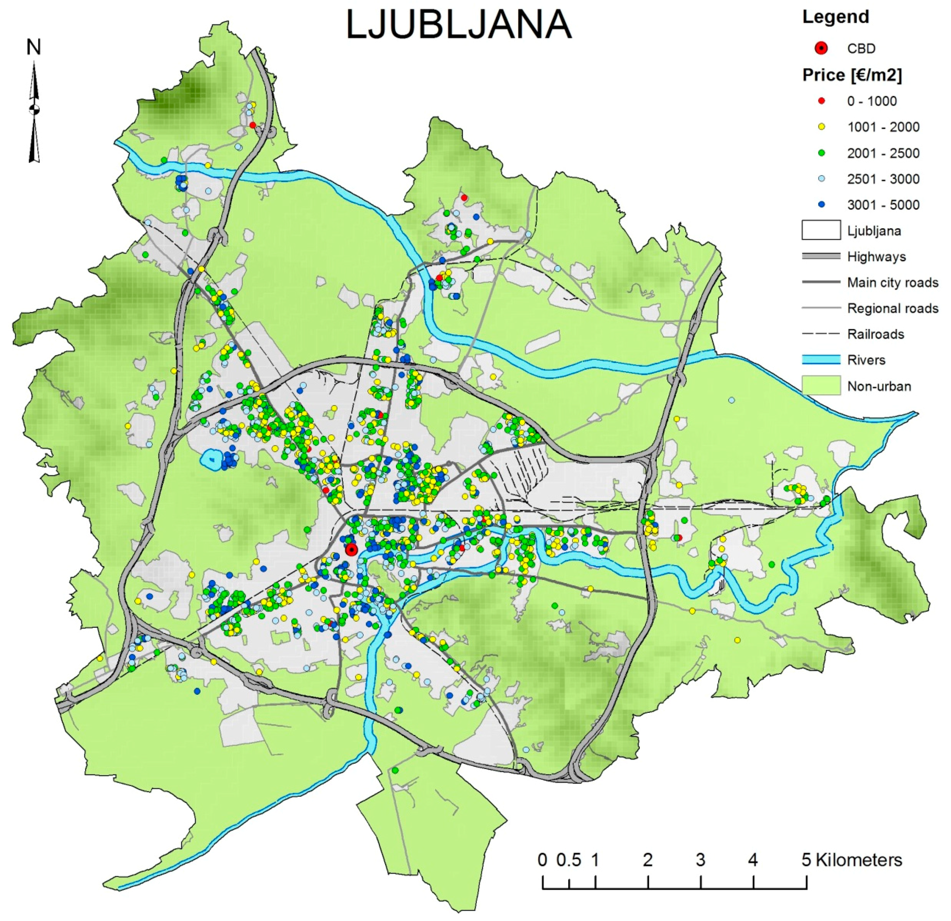
2. Case Study and Data Description

Ljubljana is the capital city of the Republic of Slovenia and is situated at the confluence of the Ljubljanica River and Sava River in central Slovenia. The administrative boundary of the city of Ljubljana encompasses 275 km² and has nearly 300,000 inhabitants in 40 settlements. The city morphology is very complex, since green wedges of forests and meadows on low hills, which serve as two large city parks, are incised towards the Central Business District (CBD) from the west and southeast (Figure 1). Regions of semi-agricultural, small gardens and recreational areas extend towards densely urbanised settlements in the center from the northeast and northwest.

Slovenian real estate prices peaked in the first half of 2008. In the study period of this analysis, which is from the year 2008 to the end of 2013, the prices of apartments in Ljubljana declined by a total of 28%, which represents the deepest fall in the Slovenian real estate market.

The original data set of 7407 records of apartment transactions, provided by the Mass Real Estate Valuation Office at the Surveying and Mapping Authority of the Republic of Slovenia, refers to real estate sales from 2008–2013, a period of six consecutive years. The transaction records are geocoded and include total transaction prices (€) and structural, time, environmental and neighbourhood information. The mean value of observed transactions is 2415 €, the minimum is 711 € and the maximum is 4934 € with a standard deviation of 575 € per square meter.

Explanatory Variables

When predicting prices as a dependent variable in the real estate market, the determinants of apartment prices can be divided into four groups [19]: (1) time/structural variables (e.g., age, the number of rooms in each house, etc.); (2) accessibility variables (e.g., the proximity of schools, bus routes, railway stations, shops, parks, and the Central Business District); (3) neighbourhood variables (e.g., local unemployment rates); (4) environmental variables (e.g., road noise and visibility impact).

In accordance with this apportionment, all available explanatory variables in our study were divided into those four groups (

Table 1. The list of explanatory variables used in study with corresponding variance inflation factor (VIF) values.

Variables	Description	Type	VIF
ID_cadas_com	Unique cadastral community ID	neighborhood	2.0803
ID_building	Building ID within cadas. community	neighborhood	1.6505
ID_appartment	Apartment ID within a building	structural	1.3362
floors_total	Total number of floors in the building	structural	4.2064
year built	Year of construction	time/structural	1.1748
year_ren_roof	Year of roof replacement	time/structural	3.1731
year_ren_face	Year of facade insulation	time/structural	1.4340
constr_type	Construction type (brick, concrete, wood)	structural	2.0259
Elevator	Elevator	structural	1.0439
house_type	Housing type (single, double, raw)	structural	2.8378
no_appart	Number of apartments in building	structural	1.0815
Northing	N coordinate (mathematical)	neighborhood	2.4851
Easting	E coordinate (mathematical)	neighborhood	667.249 *
trans_date	Date of transaction (contract)	time	46.5974 *
market zone	Real estate market zone	neighborhood	1.0117
floor_appartment	Apartment floor number	structural	1.8006
position_type	Position in building (basement, ground, middle, penthouse)	structural	7.4933 *
Duplex	Apartment in 2 floors	structural	1.4334
Rooms	Number of rooms in apartment	structural	1.0680
living_area	Apartment living area	structural	2.5412
total area	Apartment total area	structural	11.3511 *
year_ren_wind	Year of windows replacement	time/structural	9.6525 *
year_ren_inst	Year of installation replacement	time/structural	2.0041
floor_above_ground	Apartment above ground floor	structural	2.4321
dist_Airport	Prox. (Euclidian distance) to airport	accessability	5.2100 *
dist_Public transport	Prox. to city bus station	accessability	726.2465 *
Elevation	Elevation above sea level	environmental	2.1488
dist_Schools	Prox. to university facilities	accessability	6.8582 *
dist_Highway entr.	Prox. to highway entrance	accessability	1.2613
dist_Highway	Prox. to highway lane	environmental	68.622 *
dist_Railway	Prox. to railway	environmental	67.061 *
dist_Recreation	Prox. to green areas, forest	accessability	2.0475
dist_Main roads	Prox. to main city roads	accessability	3.5815
dist_Regional road	Prox. to regional roads	accessability	5.5086 *
dist_River	Prox. to river banks	environmental	3.3402

* VIF > 5; variable indicates high multicollinearity.

). The explanatory variables referring to accessibility and environment could be considered to be spatial determinants [5]. They were prepared as input grids with 20 m resolution using a proximity function within the SAGA (System for Automated Geoscientific Analyses) GIS environment (http://www.saga-gis.org/). The values assigned to each of the grid cells were calculated as Euclidean distances between each cell and the input features (airport, roads, recreation areas, etc.).

3. Methods

3.1. Hedonic Price Model

The theoretical foundation of the hedonic model is based on Lancaster’s theory of consumer demand [20]. Consumers make their purchasing decisions based on the number of good characteristics as well as the per unit cost of each characteristic. Rosen [21] was the first to present a theory of hedonic pricing. An item can be valued by its characteristics; an item’s total price can be considered as a sum of the price of each of its homogeneous attributes, where each attribute has a unique implicit price in an equilibrium market. This implies that an item’s price can be regressed on the characteristics to determine the way in which each characteristic uniquely contributes to the overall composite unit price.

The ordinary least squares (OLS) linear regression is the standard method used to build hedonic price models. The basic hedonic price function can be represented as [22]:

$$\mathrm{Y}=f\left(\mathrm{S}\mathsf{\beta },\mathrm{N}\mathsf{\gamma }\right)+\mathsf{\epsilon }$$

(1)

where Y is a vector of observed housing values; S is a matrix of structural characteristics of properties; N is a matrix of time/structural variables, accessibility variables, neighbourhood variables and environmental variables; β and γ are the parameter vectors corresponding to S and N; and ε is a vector of random error terms.

The given formula can be expressed like a common regression function:

$$\mathrm{Y}=\mathrm{X}\mathsf{\beta }+\mathsf{\epsilon }$$

(2)

where Y represents n × 1 vector of n observed apartment prices, X is an n × m matrix containing explanatory variables. β is an m × 1 vector of unknown regression coefficients, and ε is a vector representing the error term.

By using an ordinary least squares solution (OLS), the unknown regression coefficients are calculated as:

$$\widehat{\beta }={({\mathrm{X}}^T\mathrm{X})}^{-1}{\mathrm{X}}^T\mathrm{Y}$$

(3)

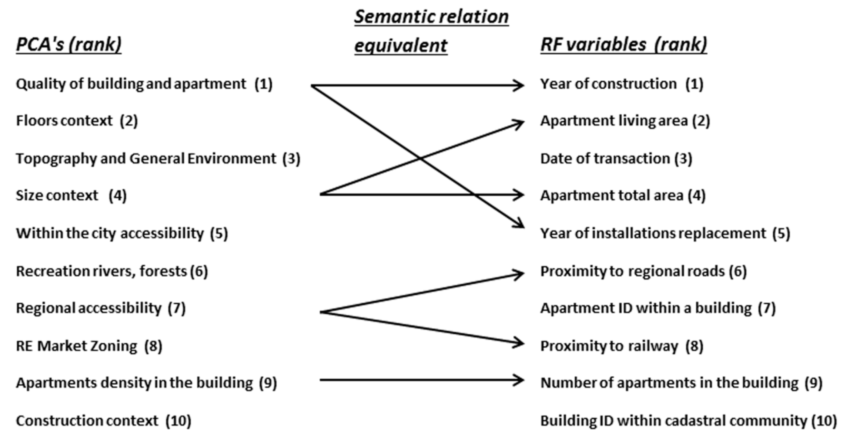
3.2. Principal Component Analysis

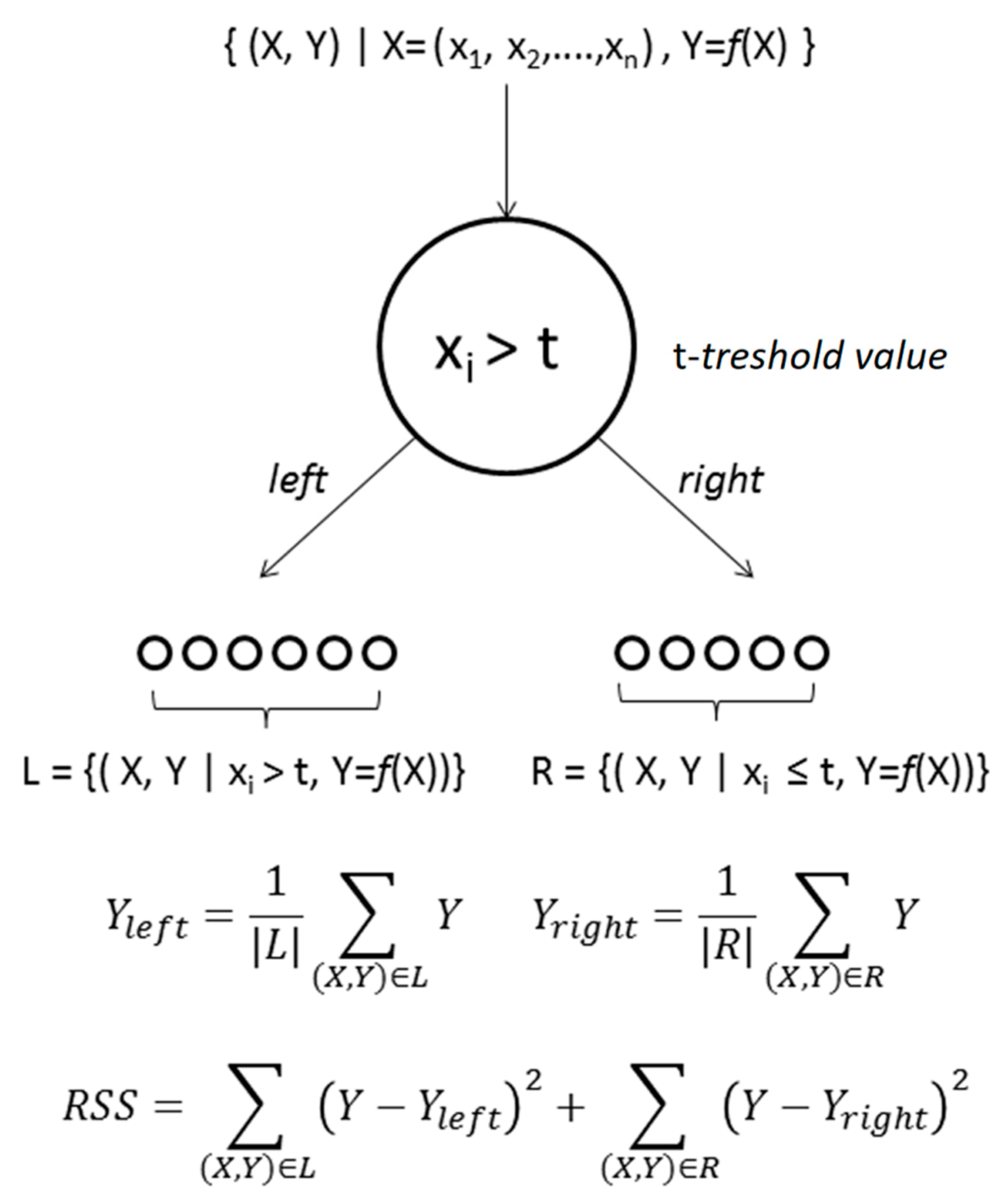
An indicator of multicollinearity between explanatory variables was inspected prior to performing the regression analysis. The variance inflation factor (VIF) test [23] indicates the presence of multicollinearity between predictors (Table 1). High multicollinearity might be a problem since it increases the variance of coefficient estimates and makes the estimates very sensitive to minor changes in the model. The resulting instability of coefficient estimates makes it difficult to interpret models. Principal Components Analysis (PCA) is often used with the aim of transforming a dataset with many intercorrelated variables (that are probably redundant) into a dataset consisting of a smaller number of uncorrelated variables, which are known as principal components (PCs) [19]. However, the main shortcoming of using PCA is that the newly generated components complicate the interpretation of the influence of the original variables. In our study, the interpretations of newly generated components of the original variables were expressed with the general real estate concepts (type of construction, age—quality of building and apartment, floors, topography and environment, size, accessibility, zoning and density)

Based on the Kaiser–Harris principle [24], only PCs with eigenvalues greater than 1 were retained, whereas the PCs with eigenvalues less than 1 explain less variance than a single explanatory variable.

3.3. Random Forest

Random forest [16] is a classification and regression algorithm based on the bagging [25] and random subspace methods [26]. The idea of bagging is to construct an ensemble of learners, each trained on a bootstrap sample (Db) obtained from the original dataset (D) using the following sampling procedure: given a D with N examples, one creates a Db by randomly choosing k examples from D with replacement (after selecting an example, it is immediately returned to D and can be selected again). After removing duplicates, if N is large and k = N, it is expected that Db contains approximately two-thirds of examples from D. The prediction of the ensemble is constructed from the separate decisions by majority voting (classification) or averaging (regression). It has been shown that bagging can reduce the variance in the final model when compared to the base models and can also avoid overfitting [25].

Regression trees are used as base learners in the RF regression algorithm. After selecting the number of trees in the forest, each regression tree is grown on a separate bootstrap sample derived from the initial training data. Each node in a tree represents a binary test against the selected predictor variable. The variable is selected to minimize the residual sum of squares for the examples flowing down both branches (left and right) (Figure 2). Terminal nodes contain no more than the specified maximal number of examples from which the target value is obtained by averaging. In order to avoid high correlations among the trees in a forest, a procedure of selecting the best splitting predictor in each node of a tree is modified to choose between only m randomly selected predictors—selecting a random subspace of the original n-dimensional problem. For a fixed parameter, m (m << n), the R package randomForest [27] uses m = n/3 by default when dealing with regression problems.

RF does not require an external cross-validation procedure to estimate the model accuracy. The example in the training data is not in the bootstrap sample containing about one third of the trees (the example is “out of bag”—OOB). Averaging the predictions of these trees produces the RF prediction on the example. The mean squared error (MSE) on the OOB samples gives the estimate for the general MSE on a separate test set. In addition, OOB can be used to estimate the i-th predictor variable’s importance by the following manner: (1) make a random permutation of values for the variable concerning the examples from the OOB, and then (2) record the increase in the MSE for the permuted OOB when compared to the original one. Here, an assumption is made that a more important variable, when permuted, will produce a greater increase in MSE when using the same regression model.

3.4. Model Performance Measures

The predicted prices of the apartments obtained by both models were compared with the observed prices in order to determine which model gives better prediction. In real estate valuation, the average sales ratio is often used as a basic measure for the evaluation of the model’s performance. The sales ratio (SR) represents the quotient between the predicted price and actual sale price for the particular apartment. However, due to the lack of normality distribution of SRs, the coefficient of dispersion (COD) is recommended for the assessment of the model prediction’s accuracy [28].

COD assesses the accuracy of the predictive model by measuring how closely each sales ratio is arrayed around the median sales ratio. The COD can be calculated using

$$\mathrm{COD}=\frac{100}{S{R}_m}\left(\frac{{\sum }_{i=1}^n\left|S{R}_i-S{R}_m\right|}{n}\right)$$

(4)

where SR_i is the sales ratio for each apartment, SR_m is the median sales ratio and n is the number of predicted apartment prices. The agreeable COD values for single-family homes and condominiums, according to the Guidance on International Mass Appraisal and Related Tax Policy document [29] range from 5% to 15%.

The mean average percentage error (MAPE) was also used to appraise the performance of the considered models:

$$\mathrm{MAPE}=\frac{100}{n}{\sum }_{t=1}^n\left|\frac{A_t-F_t}{F_t}\right|,$$

(5)

where A_t is the actual price value, and F_t is the predicted value.

3.5. R Language Environment

All of the utilized methods were implemented using the open-source R statistical computing environment with the following packages: randomForest [27] for classification and regression based on a forest of trees using random inputs, caret [30] for data splitting and generating stratified bootstrap samples, gstat for cross validation, psych for principal component analysis, as well as the sp package which provides classes and methods for dealing with spatial data in R. The results obtained in R can easily be converted into any of the standard GIS formats, which enables the manipulation and analysis of the results in commercial GIS packages afterwards.

4. Results and Discussion

4.1. OLS Model Interpretation

Before performing PCA on the set of explanatory variables, the whole data set was preprocessed, which included scaling, standardization and label encoding transformation of each categorical variable with n possible values into n binary values. The PC predictors were derived, and 10 PCs were selected in accordance with expected eigenvalues higher than 1 (Kaiser–Harris principle). The list of retained principal components is given in

Table 2. The list of component loadings (PCis) and correlations to observed explanatory variables.

Variables	PC1	PC2	PC3	PC4	PC5	PC6	PC7	PC8	PC9	PC10	h2
ID_cadas_com	−0.04	0.01	−0.05	0	0.09	0.84	0.09	−0.03	0	0.02	0.72
ID_builing	0.27	0.1	−0.25	0.05	0.1	0.16	−0.12	0.31	−0.6	−0.02	0.65
ID_appartment	0.07	0.23	−0.07	0	−0.06	0.02	−0.05	0.22	0.52	0.01	0.39
floors_total	0.05	0.83	0.05	−0.09	−0.14	0.1	0.03	−0.02	0.22	−0.08	0.78
floor_entrance	0	0.27	0.25	0	−0.22	0.05	0.17	−0.1	−0.05	0.22	0.28
year built	0.85	0.11	0	−0.03	0.13	0.04	−0.12	0	0.04	−0.01	0.76
year_ren_roof	0.62	−0.04	0.02	0.05	0.04	−0.09	−0.05	0.02	−0.08	−0.04	0.41
year_ren_face	0.75	0.1	0.06	−0.01	0.09	−0.12	−0.08	0.07	−0.02	−0.05	0.62
constr_type	−0.05	0.03	−0.06	−0.05	−0.02	0	0.04	−0.07	−0.1	0.64	0.44
elevator	0.28	0.7	0.07	0.01	−0.03	0.06	0.15	0.02	0.05	−0.09	0.61
house_type	−0.03	−0.07	0.12	0.04	−0.08	−0.04	0.09	−0.03	−0.08	0.51	0.31
no_appart	0.13	0.55	−0.11	−0.15	−0.07	0.01	−0.11	0.19	0.53	−0.14	0.71
northing	0.08	0.07	0.84	−0.03	0.3	0.09	−0.1	−0.16	0.14	−0.03	0.88
easting	−0.04	0.09	−0.49	−0.06	0.19	0.19	0.25	−0.41	0.42	0.05	0.73
trans_date	−0.03	0.02	0.07	−0.03	−0.03	−0.05	0.09	−0.04	−0.16	−0.46	0.26
market zone	−0.02	0.05	−0.07	−0.12	−0.09	0.16	−0.19	0.71	0.01	−0.09	0.6
floor_appartment	−0.03	0.91	0.02	−0.02	−0.05	0.02	−0.01	−0.02	0.02	−0.01	0.83
postion_type	−0.04	0.4	−0.02	0.05	−0.02	−0.06	−0.02	0	−0.29	0.15	0.28
duplex	0.02	−0.02	0	0.32	0.03	0	−0.02	−0.01	−0.1	0.05	0.12
rooms	0.02	−0.03	−0.01	0.85	0.02	−0.01	0	−0.02	0.06	−0.02	0.73
living_area	−0.02	−0.01	0	0.95	−0.02	−0.02	0.08	−0.02	0.02	−0.02	0.92
total area	0.02	−0.02	0	0.94	−0.01	−0.02	0.09	0	0.02	−0.02	0.89
year_ren_wind	0.83	0.01	0.01	0	0.02	0.06	−0.02	−0.05	0.04	0.05	0.7
year_ren_inst	0.86	0	0.01	0.02	0.06	0.03	−0.02	−0.02	0.05	0.06	0.75
floor_above_ground	−0.05	0.81	0	−0.03	−0.01	−0.03	−0.07	−0.01	0.04	−0.04	0.67
dist_Airport	−0.07	−0.06	−0.92	0.01	−0.17	−0.06	0.13	0.06	−0.04	0.04	0.91
dist_Public transport	0.1	−0.04	0.06	0.01	0.72	−0.02	0.11	−0.12	−0.12	−0.07	0.59
Elevation	−0.02	−0.01	0.82	0.04	−0.09	0.05	−0.22	0.29	−0.16	0.02	0.84
dist_Schools	0.15	−0.09	−0.07	0.05	0.34	−0.08	−0.05	0.26	−0.02	0.34	0.35
dist_Highway entr.	−0.13	−0.01	−0.24	0.08	0.05	−0.01	0.92	−0.13	−0.01	0.02	0.94
dist_Highway	−0.14	0.02	−0.24	0.06	−0.02	0.01	0.91	−0.12	0.01	0.02	0.93
dist_Railway	0.04	−0.09	0.26	0.06	0.21	−0.29	−0.02	0.54	0.2	0.08	0.54
dist_Recreation	0.08	−0.04	0.07	−0.01	0.75	0.33	−0.2	−0.05	0.01	−0.06	0.73
dist_Main roads	0.12	−0.17	0.2	0.05	0.82	−0.22	0.09	0.12	0.04	0.04	0.84
dist_Regional road	−0.23	0.07	0.09	0	−0.49	−0.07	0.5	0.5	0.04	0	0.81
dist_River	−0.07	0.08	0.42	−0.06	−0.13	0.74	−0.17	0.08	0	0	0.79
SS loadings	3.44	3.38	3.07	2.71	2.49	2.34	1.67	1.66	1.4	1.15
Proportion Var	0.1	0.09	0.09	0.08	0.07	0.07	0.05	0.05	0.04	0.03

.

The column labelled PCi contains the component loadings, which represent the correlations of the observed explanatory variables with the principal components. Component loadings are used to interpret the meaning of the components. The dark shaded table cells indicate strong correlations (over 0.60), while light shaded cells specify high or moderate correlations between the PCi and explanatory variable. The column labelled h2 contains the component communalities, which represent the amount of variance in a variable explained by the components (the proportion of each variable’s variance can be explained by the principal components).

The row labelled SS loadings contains the eigenvalues associated with the components. An eigenvalue is the standardized variance associated with a particular component (in this case, the value for the first component is 3.44). The row labelled Proportion Var represents the amount of variance accounted for by each component. Here, it can be seen that the first principal component, PCA1, includes a number of variables with high loadings and accounts for 10 percent of the variance in the 36 variables.

Component loadings indicate the relative contribution of the observed variables to each principal component, which can help in the interpretation of the meaning of PCAs in real-word settings.

Concerning component loadings for PC1 and strong correlations with predictors such as year of installations (pipelines, wires) replacement, year of construction, year of window replacement, year of facade insulation and year of roof replacement, PC1 could be interpreted as “age—quality of building and apartment”.

Due to its strong correlation to the apartment floor number, total number of floors in the building, apartment floor number (starting above the ground floor) and number of apartments in the building, PC2 is interpreted as “floors”.

PC3 is strongly positively correlated with the elevation of the building itself above sea level, the northing Y coordinate and the proximity to river banks, and negatively correlated with the easting X coordinate and the proximity to the airport.

The threat of flooding has been noted in Ljubljana, and buildings above common flood levels are highly valued. The main city business development axis is directed towards the north, which is followed by spatial price trends of housing. On the other hand, the Eastern part of the city is more industrialized, and a huge railway arrangement area extends from the downtown core to the Eastern direction. Distance to an airport (noise), as an environmental element, influences the prices negatively. The proximity to riverbanks and the lake shore, as an environmental amenity, influences apartment prices positively. PC3 is interpreted as “topography and general Environment”.

Due to its high component loadings on the apartment living area, apartment total area and number of rooms in an apartment, PC4 is recognized as the “Size” context.

PC5 has a high positive correlation with proximity to main city roads, distance to green areas such as forests, proximity to “city bus lines” stations, distance to university facilities, and its negative correlation with the distance from regional roads, and for that reason, can be interpreted as “accessibility within the city”.

PC6 is interpreted as the recreation rivers and forests context with respect to its high component loadings of distances to river banks and distances to green areas and forest. The river courses and forest boundaries coincide with cadastral community boundaries and for that reason, this principal component also has a strong correlation with cadastral community IDs.

An exceptionally high correlation (>0.9) with the distance to highway entrances and the distance to highway lane makes PC7 the “regional accessibility” context.

Provided that railway corridors represent the boundaries of real estate market zones in Ljubljana and that PC8 has a high correlation with the real estate market zoning and the distance to the railway, PCA8 is interpreted as “RE market zoning”.

PC9 is interpreted as “apartment density in the building” due to its correlation with the number of apartments in a building and the apartment ID within a building. Apartments IDs grow from the bottom to the top of a building.

PC10 is interpreted as the “construction” context owing to its component loading values of construction type (brick, concrete, wood) and housing type (single, double, raw houses).

The date of transaction is a time specific variable and indicates no significant correlation to any of the PCA components, which implies that the regression model in our case does not take into account the price differences over the considered time period. The summary output of the multiple regression model on the PCAs shows that the model explains only 23% of the variability and is statistically significant.

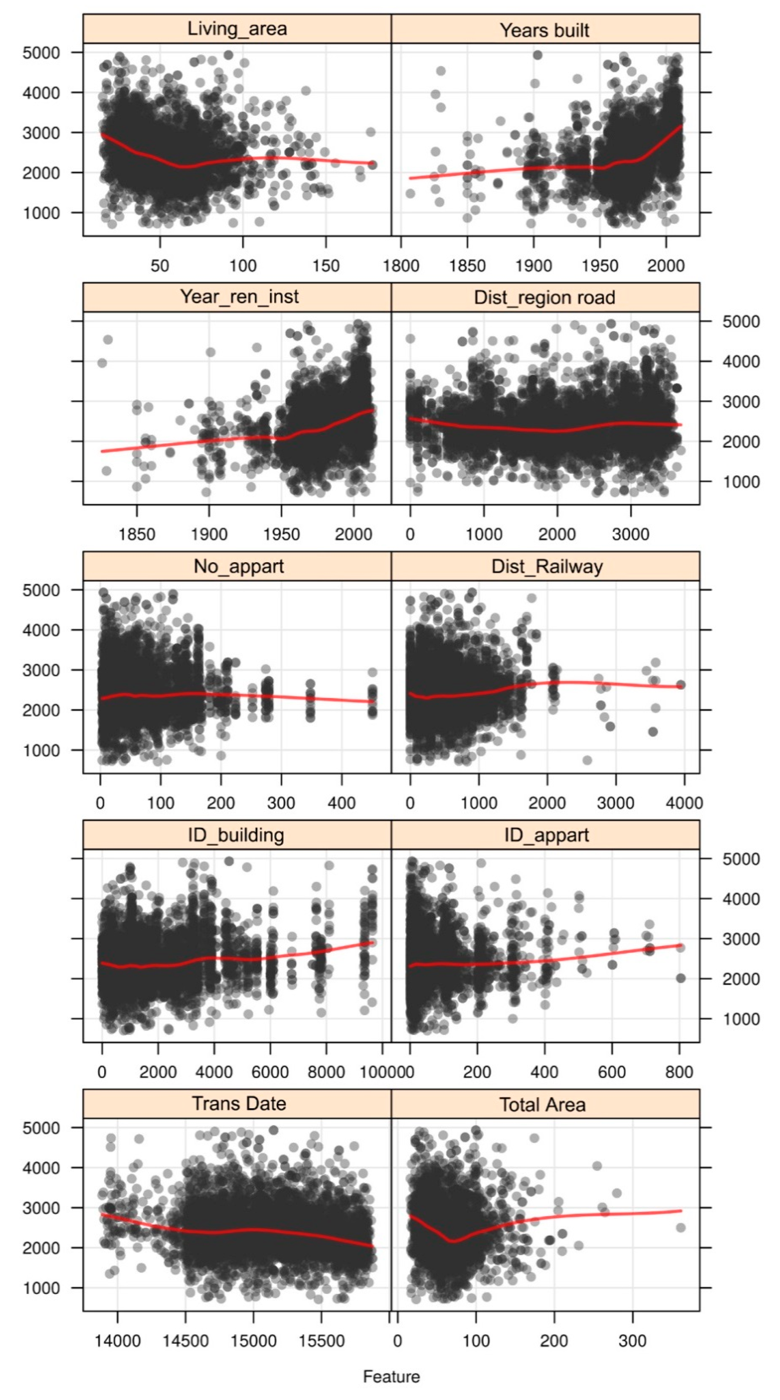
4.2. Random Forest Model Interpretation

Similar to the application method of the multiple regression model, we examined the importance of the predicting variables calculated from permuting the OOB data. We decided to only use the first ten ranked predictors (Figure 3) out of 36 by using a trial and error method to build the RF model on training data (70% bootstrap sample).

The scatter plots (Figure 3) were used in order to depict a bivariate relationship (predictors’ values versus price/m²). Since the overlap of data points in scatter plots makes it difficult to discern the relationship, a smoothed curve through the cloud of points was fitted to describe the general relationship between the variables and apartment prices.

The interpretation of the relationships between particular variables and apartment price is given in ranked order of importance:

1. Year built (year of construction): recently built apartments have higher prices per m², in general. Nowadays, prices for apartments in buildings built from the year 1900 to the period before the end of World War II (WW2) have risen. The prices are lower for apartments in the buildings built in the period just after WW2 as the economic standard of living at that period was low and consequently, a lower quality of construction generally appeared in Slovenia and in Ljubljana. Apartment prices of buildings built after 1950, rising from an average of 2100 €/m² up to 3200 €/m² for newly-built buildings.

2. Living_area (apartment living area): smaller apartment living areas (studios and one room apartments for young couples or single households are most frequently exchanged on the market) indicate a higher price per square meter. The price per m² of an apartment declines from around 3000 €/m² to about 2100 €/m² for smaller living area between 20 m² and 65 m² in Ljubljana (19.5 €/m² for each additional m² on above mentioned interval). Apartment prices then rapidly rise per each additional m² of living area, up to 2300 €/m² (for 115 m² apartments), which might indicate the apartment market of higher income households of families with kids and both parents employed. Larger apartments (from 115 m² to 200 m²) decline in their value per square meter for each additional m².

3. Trans_date (date of transaction): represents the change in price/m² in time (days) on the relative timescale from the beginning of 2008 until the middle of 2013 (1989 days)—a period of recession in Slovenia. The graph of price changes corresponds to the reported decline of the market price, from about 3000 €/m² to about 2000 €/m² in four and a half years.

4. Total_area (Aaartment total area): represents the sum of an apartment’s living area and the additional area for storage and the balcony. It is highly correlated by the predictor, apartment living area. For that reason, changes in price/m² have approximately the same trend as the apartment living area but the influence of an enlarged area is reduced by about 200 €/m².

5. Year_ren_inst (year of installations’ replacement): The utilities and installations in the apartment physically deteriorate or depreciate over time and must be replaced. The younger the replacements are, the higher the average price/m² of apartments in the sample is. Apartments with old installations have an average price of 1700 €/m², whereas apartments with new replacements of gas, electrical and plumbing installations have an average price of 2800 €/m².

6. Dist_Reginal road (proximity to regional roads) Regional roads bring traffic to the city of Ljubljana from surrounding regions and are connected to the ring motorway built around the city. Their influence on the housing price decreases slightly at up to 2 km of distance and then increases to a distance of approximately 3 km. The price then decreases again over larger distances from the ring motorway.

The decline in average prices from 2600 €/m² to 2300 €/m² compared to the growing distance from regional roads might be understood as a negative influence of increased walking distances to public transportation flow, which is usually located along regional roads.

7. ID_apartment (apartment ID within a building): apartments in Slovenia are strictly numbered from the bottom to the top of the building. The prices are fairly constant with the growing number of apartment ID but begin to plateau at around ID number 300. Only high rise condominiums have apartment IDs over 300. Slightly growing prices above building unit 300 represent top floor positions of apartments in the buildings and penthouse positions with excellent views over lower condominiums. In Ljubljana, these higher positions mean beautiful views over the Kamnik–Savinja Alps mountain range to the north or views onto the nice medieval city centre and Castle Hill, surrounded by the river Ljubljanica. This predictor is, as expected, correlated with the predictors, nu_flt_in_build (number of apartments in the building), flt_floor (apartment floor number) and flt_floor_base (number of apartments above the ground floor). There are some underground and half underground apartments which are not desirable on the market and therefore, they do not reach high prices.

8. Dist_Railway (proximity to railway) In general, apartments closer to railroad yield lower prices; the average price/m² closer to railroads is about 2250 €/m² and the (environmental noise) influence of railroad proximity to housing disappears after about 1.5 km, where the average prices are above 2.700 €/m² in Ljubljana. However, there is special situation in Ljubljana, where degraded land and abandoned buildings in several locations close to railroads were recently replaced by modern condominiums with high quality construction with the average price at around 2400 €/m².

9. No_apart (Number of apartments in the building): the price/m² grows from 2100 €/m² to about 2300 €/m² for buildings with up to 20 apartments. In this building size, about 83% of the 1550 buildings are not equipped with an elevator. The remaining 17% of the buildings have higher apartment prices. From 20 to about 100 apartments per building, the price is almost stabilised. However, the price/m² declines for buildings with huge numbers of apartments.

10. ID_building (building ID within cadastral community): new buildings have the largest available number in the sequence within the cadastral community, and apartment prices/m² for newly built structures are higher than older ones. However, there is an anomaly in the graph for the interval from approximately ID 3000 to ID 5000, which is the result of random chance. The ID numbers of buildings from the abovementioned interval (in four cadastral communities) correspond to the neighbourhoods of higher prices (Zupančičeva jama, Trnovski bloki, Vič south of Cesta na Brdo and Šiška elite settlement Koseze pond).

Comparing, semantically, the set of interpretations of the top ten PCAs with the set of top ten ranked predictors selected by RF (importance calculated from permuting OOB data), we can conclude that the two models have equivalent ratings for 7 out of 10 variables (Figure 4).

4.3. The Comparison of OLS and RF Performance

The comparison of OLS and RF performance was conducted in an out of sample prediction context using a stratified five-fold cross validation procedure with training sets consisting of 70% of all transactions and test sets consisting of 30% of all transactions. In “stratified” cross-validation, training and test sets have the same spatial and price value distribution as the full dataset [31]. In addition, “stratified” is a variant of the k-fold within training data and also ensures that each fold has the right proportion of samples in regard to spatial location and price values.

Predefined performance measures for both sets of data are given in

Table 3. Prediction accuracy for ordinary least square (OLS) and RF training and test data sets.

	OLS		RF
	Train	Test	Train	Test
SR	1.0447	1.0465	1.0191	1.0197
MAPE [%]	16.85	17.48	7.04	7.27
COD [%]	16.52	17.12	7.05	7.28
R2	0.23		0.57

. All performance measures (SR, MAPE, COD) indicate that significantly better results were obtained by RF in comparison to OLS. Considering the R² values for OLS and RF (0.23 and 0.57, respectively) and the noticeably lower MAPE and COD values for the RF model, it can be concluded that we are facing a non-linear problem. RF outperforms the OLS model in this non-linear situation; even COD values for OLS are above the recommended upper limit (17% > 15%). The obtained results for the sales ratio (SR) were adequate for both applied methods for both the training and test data sets in accordance with the approved range of 0.9–1.1 [29].

The effects of predictions performed by two methods were also compared by detailed visual inspection of differences between the sales ratios (SR) of OLS and RF predictions at identical locations. Figure 5a. shows the kernel density [32] of the differences between the average sales ratio values of the OLS and RF models for the apartments in each building (SR(OLS)—SR (RF)). The spatial distribution of the kernel density of sales ratio differences is shown within seven classes, from −0.100 to 0.100 (from dark brown to azzuro blue, middle class is transparent). The locations representing positively signed differences between sales ratios of OLS and RF assessments, coloured azzuro blue, are predominantly situated at the north of the CBD (north, northeast and northwest), which are the main directions of business activity development. They are also located in smaller quantity towards the east (at the confluence of the river Ljubljanica) and southwest and are radially dispersed from the CBD along the regional connecting roads.

Most interesting is the distribution of negatively signed differences between the average sales ratios (RF sales ratios values are higher than OLS sales ratios). The locations of negative differences represent contemporary settlements of apartments, and they are marked by a red check mark symbol (Figure 5a).

In order to obtain more insight into how the prediction models behave over the case study area, the Hot Spot Analysis was performed by calculating Getis–Ord Gi statistics [33]. The best way to interpret the Getis–Ord Gi statistic is in the context of the standardized Z-score values. A positive Z-score of Gi statistics (red points, H-H, high clustering of high values) appears when the spatial clustering is formed by similar, but high, values (in our case average SR > 1). If the spatial clustering is formed by low values (in our case average SR < 1), the Z-score (blue points, L-L, high clustering of low values) tends to be negative. A Z-score of around 0 (transparent points, Insignificant clustering) indicates no apparent spatial association pattern.

The hot spot spatial clusters of average SR were mapped over the massive appraisal map obtained by kriging interpolation of the considered transactions (Figure 5b,c).

It is obvious that both models followed similar spatial patterns over the case study area. Both methods underestimated the higher prices of apartments (SR < 1, blue points over orange areas), and overestimated the lower prices of apartments (SR > 1, red points over light green areas).

By coupling the results of the Hot Spot Analysis results with the kernel density of the difference between average SRs for OLS and RF, it is evident that blue points where RF underestimated actual prices are coincided with dark brown areas (areas where SR(RF) > SR(OLS)). Therefore, it can be concluded that RF predictions are closer to actual prices than OLS predictions in those areas. Those particular areas are the CBD area as well as areas with contemporary locations, i.e., the areas with high apartment prices.

On the basis of the above facts, and considering the obtained performance metrics, it is suggested that RF predictions outperform OLS predictions. Namely, at the locations of higher differences in sales ratios (where the values are slightly higher), the RF model shows more sensitivity than the OLS model for capturing differences in values.

5. Conclusions

The objective of this research was to empirically compare the predictive power of the OLS hedonic model with a random forest model for predicting apartment prices in Ljubljana, for the period between 2008 and 2013.

Before OLS modelling was performed, the initial set of 36 predicting variables was transformed into a Principal Components Analysis feature space in order to avoid immanent multicollinearity between variables. The 10 extracted PCAs were analysed by component loadings and clustering of initial explanatory variables in the component space in order to obtain an interpretation and semantic description in the original feature space.

Analogous to the OLS model, the random forest (RF) and out of the bag (OOB) permuting error estimate was adopted to select 10 of the most important predicting variables that were used for RF modelling.

We discovered a relatively high rate of equivalent semantic relationships (approximately 70%) between the set of interpretations of the top ten PCAs with the set of top ten ranked predictors selected by RF.

The commonly applied adjustment of prices over time for the sales data was purposely skipped in order to examine the sensitivity of the predictive models to the influence of time variability. Hence, the time period with the greatest change of prices in Slovenia, the six consecutive years between 2008 and 2013 that showed a 28% decline, was chosen for this research. The OLS model did not account for the time specific variable, “date of transaction”, which represents the basic information for adjustment of prices over time. However, the “date of transaction” variable was considered strongly by RF and was determined to be the third most influential variable and is effectively used for time adjustment.

All performance measure—R² values (0.23 for OLS and 0.57 for RF), the sales ratios (1.04 for OLS and 1.02 for RF), the MAPE (17% for OLS and 7% for RF) and the COD (17% for OLS and 7% for RF)—revealed significantly better results with random forest. The low R² value for the OLS model indicated that non-linear modelling was required.

Visual inspection of the differences between the sales ratios (SR) of the OLS and RF predictions showed that the models perform similarly at identical locations. Both methods underestimated the higher prices of apartments (SR < 1) and overestimated the lower prices of apartments (SR > 1). However, we found that the RF predictions were closer to actual prices than the OLS predictions by combining results of kernel density for the differences of average of sales ratios between OLS and RF (SR (OLS)-SR (RF)) for the apartments in the buildings and the results of the Hot Spot Analysis. In addition, negative values of differences between the average SR (sales ratios of RF are larger than OLS sales ratios) were located at the spots where elite groups of condominium buildings are raised. Apartments in these specific locations would be under-valued using OLS predictions. In contrast, RF captures their differences due to amenities attributed to them.

Finally, the entire analysis of the spatial distribution of sales ratios for both methods has revealed that the random forest algorithm could provide better detection of the variability in apartment values and predicts them more effectively than multiple regression in complex urban forms like the city of Ljubljana, Slovenia.

References

1. Lake, I.R.; Lovett, A.A.; Bateman, I.J.; Day, B. Using GIS and large-scale digital data to implement hedonic pricing studies. Int. J. Geogr. Inf. Sci. 2000, 14, 521–541. [Google Scholar] [CrossRef]
2. Din, A.; Hoesli, M.; Bender, A. Environmental variables and real estate prices. Urban. Stud. 2001, 38, 1989–2000. [Google Scholar] [CrossRef]
3. Zhang, Y.; Dong, R. Impacts of Street-Visible Greenery on Housing Prices: Evidence from a Hedonic Price Model and a Massive Street View Image Dataset in Beijing. ISPRS Int. J. Geo-Inf. 2018, 7, 104. [Google Scholar] [CrossRef]
4. Schernthanner, H.; Asche, H.; Gonschorek, J.; Scheele, L. Spatial modeling and geovisualization of rental prices for real estate portals. In Computational Science and Its Applications—ICCSA 2016; Gervasi, O., Ed.; Springer: Cham, Switzerland, 2016; Volume 9788. [Google Scholar] [CrossRef]
5. Bajat, B.; Kilibarda, M.; Pejović, M.; Samardžić Petrović, M. Spatial Hedonic Modeling of Housing Prices Using Auxiliary Maps. In Spatial Analysis and Location Modeling in Urban and Regional Systems; Thill, J.C., Ed.; Springer: Berlin/Heidelberg, Germany, 2017; pp. 97–122. [Google Scholar]
6. Meen, G. Spatial housing economics: A survey. Urban. Stud. 2016, 53, 1987–2003. [Google Scholar] [CrossRef]
7. Tay, D.P.; Ho, D.K. Artificial intelligence and the mass appraisal of residential apartments. J. Prop. Valuat. Invest. 1992, 10, 525–540. [Google Scholar] [CrossRef]
8. Do, A.Q.; Grudnitski, G. A neural network approach to residential property appraisal. Real Estate Appraiser 1992, 58, 38–45. [Google Scholar]
9. Borst, R.A. Artificial neural networks in mass appraisal. J. Prop. Tax Assess. Adm. 1995, 1, 5–15. [Google Scholar]
10. Chiarazzo, V.; Caggiani, L.; Marinelli, M.; Ottomanelli, M. A Neural Network based model for real estate price estimation considering environmental quality of property location. Transp. Res. Proc. 2014, 3, 810–817. [Google Scholar] [CrossRef]
11. Yalpir, S.; Durduran, S.S.; Unel, F.B.; Yolcu, M. Creating a Valuation Map in GIS Through Artificial Neural Network Methodology: A Case Study. Acta Montan. Slovaca 2014, 19, 89–99. [Google Scholar]
12. Fan, G.Z.; Ong, S.E.; Koh, H.C. Determinants of house price: A decision tree approach. Urban. Stud. 2006, 43, 2301–2315. [Google Scholar] [CrossRef]
13. Vapnik, V. The Nature of Statistical Learning Theory; Springer: New York, NY, USA, 1995; p. 768. [Google Scholar]
14. Kontrimas, V.; Verikas, A. The mass appraisal of the real estate by computational intelligence. Appl. Soft Comput. 2011, 11, 443–448. [Google Scholar] [CrossRef]
15. Yu, D.; Wu, C. Incorporating Remote Sensing Information in Modeling House Values. Photogramm. Eng. Remote Sens. 2006, 72, 129–138. [Google Scholar] [CrossRef]
16. Breiman, L. Random forests. Mach. Learn. 2001, 45, 5–32. [Google Scholar] [CrossRef]
17. Antipov, E.A.; Pokryshevskaya, E.B. Mass appraisal of residential apartments: An application of Random forest for valuation and a CART-based approach for model diagnostics. Expert Syst. Appl. 2012, 39, 1772–1778. [Google Scholar] [CrossRef]
18. Yoo, S.; Im, J.; Wagner, J.E. Variable selection for hedonic model using machine learning approaches: A case study in Onondaga County, NY. Landsc. Urban Plan. 2012, 107, 293–306. [Google Scholar] [CrossRef]
19. Lake, I.R.; Lovett, A.A.; Bateman, I.J.; Langford, I.H. Modelling environmental influences on property prices in an urban environment. Comput. Environ. Urban. Syst. 1998, 22, 121–136. [Google Scholar] [CrossRef]
20. Lancaster, K.J. A new approach to consumer theory. J. Polit. Econ. 1966, 74, 132–157. [Google Scholar] [CrossRef]
21. Rosen, S. Hedonic Prices and Implicit Markets: Product Differentiation in Pure Competition. J. Polit. Econ. 1974, 82, 34–55. [Google Scholar] [CrossRef]
22. Se Can, A.; Megbolugbe, I. Spatial dependence and house price index construction. J. Real Estate Financ. Econ. 1997, 14, 203–222. [Google Scholar] [CrossRef]
23. Zuur, A.F.; Ieno, E.N.; Elphick, C.S. A protocol for data exploration to avoid common statistical problems. Methods Ecol. Evol. 2010, 1, 3–14. [Google Scholar] [CrossRef]
24. Kaiser, H.F. The application of electronic computers to factor analysis. Educ. Psychol. Meas. 1960, 20, 141–151. [Google Scholar] [CrossRef]
25. Breiman, L. Bagging predictors. Mach. Learn. 1996, 24, 123–140. [Google Scholar] [CrossRef]
26. Ho, T.K. The random subspace method for constructing decision forests. IEEE Trans. Pattern Anal. 1998, 20, 832–844. [Google Scholar] [CrossRef]
27. Liaw, A.; Wiener, M. Classification and regression by random Forest. R News 2002, 2, 18–22. [Google Scholar]
28. Moore, J.W. Performance comparison of automated valuation models. J. Prop. Tax Assess. Adm. 2006, 3, 43–59. [Google Scholar]
29. International Association of Assessing Officers. Guidance on International Mass Appraisal and Related Tax Policy. 2014. Available online: http://www.iaao.org/media/Standards/International_Guidance.pdf (accessed on 3 March 2018).
30. Kuhn, M. Caret package. J. Stat. Softw. 2008, 28, 1–16. [Google Scholar]
31. Orton, T.; Pringle, M.; Bishop, T. A one-step approach for modelling and mapping soil properties based on profile data sampled over varying depth intervals. Geoderma 2016, 262, 174–186. [Google Scholar] [CrossRef]
32. Silverman, B.W. Density Estimation for Statistics and Data Analysis; Chapman and Hall: New York, NY, USA, 1986; p. 175. [Google Scholar]
33. Getis, A.; Ord, J.K. The Analysis of Spatial Association by Use of Distance Statistics. Geogr. Anal. 1992, 24, 189–206. [Google Scholar] [CrossRef]
Figure 1. Observed transactions of apartments in Ljubljana in the period from 2008–2013.
Ijgi 07 00168 g001
Figure 2. Regression tree node.
Ijgi 07 00168 g002
Figure 3. The scatter plots of predictor values versus price/m2 values.
Ijgi 07 00168 g003
Figure 4. Semantic comparison of the top ten Principal Components (PCs) with the set of top ten ranked predictors selected by random forest (RF).
Ijgi 07 00168 g004
Figure 5. (a) Kernel density of the difference between sales ratios of OLS and RF; (b) Hot Spot Analysis of average sales ratio (SR)(OLS); (c) Hot Spot Analysis of average SR(RF).
Ijgi 07 00168 g005