2DPR-Tree: Two-Dimensional Priority R-Tree Algorithm for Spatial Partitioning in SpatialHadoop


1
Department of Information Systems, Kafr El-Sheikh University, Kafr El-Sheikh 33511, Egypt
2
Department of Information Systems, Mansoura University, Mansoura 35516, Egypt
*
Author to whom correspondence should be addressed.
ISPRS Int. J. Geo-Inf. 2018, 7(5), 179; https://doi.org/10.3390/ijgi7050179
Submission received: 23 March 2018
/
Revised: 1 May 2018
/
Accepted: 7 May 2018
/
Published: 9 May 2018
(This article belongs to the Special Issue Cognitive Aspects of Human-Computer Interaction for GIS)
Abstract
:Among spatial information applications, SpatialHadoop is one of the most important systems for researchers. Broad analyses prove that SpatialHadoop outperforms the traditional Hadoop in managing distinctive spatial information operations. This paper presents a Two Dimensional Priority R-Tree (2DPR-Tree) as a new partitioning technique in SpatialHadoop. The 2DPR-Tree employs a top-down approach that effectively reduces the number of partitions accessed to answer the query, which in turn improves the query performance. The results were evaluated in different scenarios using synthetic and real datasets. This paper aims to study the quality of the generated index and the spatial query performance. Compared to other state-of-the-art methods, the proposed 2DPR-Tree improves the quality of the generated index and the query execution time.
1. Introduction
The rapid and continuous growth of geospatial information generated from devices such as smartphones, satellites, and other Internet of Things (IoT) devices means that traditional Geographic Information System (GIS) cannot support such a large amount of data [1,2]. GIS is insufficient in this situation because of poor adaptability of the basic incorporated frameworks. Therefore, blending both GIS and cloud computing represents a new era for the advancement of data storage and processing, and their applications in GIS [3,4].
Recently, Hadoop [5,6] has become the most well-known open source cloud-computing platform. Hadoop provides a solution for the problem of data processing of huge datasets in many fields. Hadoop employs MapReduce [7,8,9,10] to produce an efficient data processing framework. MapReduce is a simplified distributed processing programming paradigm that has been utilized for a variety of applications, such as constructing indexes, data classification and clustering, and different types of information analysis [11]. MapReduce was developed to give an effective distributed parallel processing paradigm with a high degree of fault tolerance and adequate scalability mechanisms. However, Hadoop has some deficiencies in terms of effectiveness, especially when dealing with geospatial data [8]. A primary inadequacy is the absence of any indexing mechanism that could support specific access to spatial information in particular areas due to the demands for effective query processing. Because of this issue, an expansion of Hadoop, called SpatialHadoop, has been developed. SpatialHadoop [12,13] is a Hadoop system that is suited for spatial operations. It adds spatial constructs and geospatial information into the Hadoop core functionality.
In SpatialHadoop, spatial data are purposely fractioned and distributed to Hadoop cluster nodes. From that point, information that has spatial nearness is congregated in the same partition, which will be indexed later. All SpatialHadoop indexing structures are based on a set of partitioning techniques. All of these partitioning techniques are built-in to the Hadoop Distributed File System (HDFS). Consequently, SpatialHadoop provides efficient query processing algorithms that access just a particular area of the information and give the correct query result. As exhibited in the paper by Ahmed Eldawy and Mohamed Mokbel [12], many spatial operations are proposed, such as range query [14,15,16], kNN query [17,18], spatial joins [19,20,21], and skyline query [22].
The contributions of this paper are summarized as follows: (1) the Two-Dimensional Priority R-Tree (2DPR-Tree) is proposed as a version of the PR-Tree with some enhancements that make it applicable in SpatialHadoop. (2) Unlike other techniques, the 2DPR-Tree algorithm achieves simultaneous partitioning of the input shapes into the desired number of partitions and highly preserved spatial proximity of these shapes. (3) A broad arrangement of experiments on different datasets (synthetic and real) was executed to illustrate the efficiency and scalability of the 2DPR-Tree indexing technique. (4) Compared to other techniques, the 2DPR-Tree has a superior performance and functionality for range and kNN queries.
The rest of the paper is organized as follows: Section 2 discusses related works on SpatialHadoop and SpatialHadoop indexing techniques. Section 3 illustrates the overall architecture of SpatialHadoop. Section 4 presents a description of the Priority R-Tree (PR-Tree). Section 5 presents a description of the proposed 2DPR-Tree partitioning technique in SpatialHadoop. Section 6 presents the experimental setup, configurations, and the performance measures. The representative results of the extensive experimentation performed are also included in this section. Finally, Section 7 concludes the work and discusses future research directions.
2. Related Work
Since files in Hadoop are not indexed, they must be sequentially filtered and scanned. To overcome this issue SpatialHadoop utilizes spatial indexes inside the Hadoop Distributed File System as a method for the efficient recovery of spatial information [23]. Indexing is the key difference of SpatialHadoop in terms of achieving a better execution than Hadoop and the other systems [24].
SpatialHadoop provides various indexing algorithms that mainly differ in data partitioning techniques. As shown in Table 1, SpatialHadoop provides space partitioning techniques such as a grid and Quadtree, space-filling curve (SFC) partitioning techniques such as the Z-curve and Hilbert curve, and data partitioning techniques such as Sort-Tile-Recursive (STR), STR+, and KD-Tree [23].
The grid technique [25] is a uniform data partitioning technique. This technique divides the spatial space into equal-sized rectangles using a uniform grid of cells, where is the desired number of partitions, and data located on the boundaries between partitions are redundantly allocated to those overlapping partitions. The simple process and calculations of the grid technique allow a minimal index creation time. The grid partitioning technique is simple to implement, however it causes non-uniform data distribution through the cluster nodes. This affects load balancing and therefore the efficiency of the query. The spatial query efficiency is not optimal because of the unorganized data, and the consequent time taken to search the data for the query [26].
The Quadtree technique is a Quadtree-based data partitioning technique. It preserves the adjacent relationship of objects and provides a space uniform recursive decomposition into partitions (four partitions in each iteration) until each partition has the object’s defined number limit. Therefore, there is no way to control the generated partition number to satisfy the desired number of partitions. Similar to the grid partitioning technique, data located on the partition boundaries are redundantly allocated to those overlapping partitions. The Quadtree technique is extremely suited for parallel processing. However, high data transfer and high I/O costs are required, and it is hard to apply in higher dimensions [27].
The Z-curve technique sorts the input points based on their order on the Z-curve and then separates the curve into partitions. Boundary objects that overlap in different partitions are assigned to the partition with maximal overlap. The Z-curve technique generates almost equal sized partitions with a linear complexity of the mapper’s input, but the spatial neighborhood relationships are not always well preserved as it generates a high degree of overlap between partitions [26,28].
The Hilbert curve is a space-filling curve technique that uses the Hilbert-curve to bulk-load the R-Tree on MapReduce [29]. The partitioning function puts objects in the same partition to keep spatial proximity by using the sorted minimum boundary rectangle (MBR) values of object nodes from the Hilbert-curve, and transforms them into a standard and proven multi-dimensional index structure—R-Tree—through parallelization in MapReduce. Hilbert packing reduces the data transfer overhead through the network and thersefore the query response time [30]. Similar to the Z-curve, boundary objects that overlap in more than one partition are assigned to the maximal overlap partition.
The STR technique is an R-Tree packing algorithm [31,32]. It divides the input spatial data based on a random sample into an R-Tree [33,34] and each node in the tree has objects, where k is the random sample size and is the desired number of partitions. All leaf node boundaries are used as partition boundaries. Boundary objects that overlap in more than one partition are assigned to the maximal overlap partition.
The STR+ technique is the same as the STR technique. However, boundary objects that overlap in more than one partition are redundantly assigned to the overlapping partitions [35].
The KD-Tree technique transforms multidimensional location information into one-dimensional space. SpatialHadoop utilizes the KD-Tree partitioning method in the paper by Jon Louis Bentle [36] to partition the input dataset into partitions. The KD-Tree technique begins with the input MBR as one partition and partitions it times to produce n partitions. Boundary objects that overlap in more than one partition are redundantly assigned to overlapping partitions.
3. The Overall Architecture of SpatialHadoop
A SpatialHadoop cluster has one master node that divides a map-reduce job into smaller tasks, distributed to and executed by slave nodes. As shown in Figure 1, users access SpatialHadoop through The Pigeon Language in the Language layer to process their datasets. The Pigeon is an SQL-like language that supports the Open Geospatial Consortium (OGC) standard that was developed to simplify spatial data processing [37].
The operations layer consists of the various computational geometry operations, as mentioned in the paper by Ahmed Eldawy, et al. [9], and a set of spatial queries such as the range query and kNN query. The range query [14] takes the spatial input dataset SR and a query area QA as information and returns all objects in SR that are located within QA. In Hadoop, the input dataset is stored as a sequential heap file. Thus, all spatial input objects must be examined to get the result. SpatialHadoop attains a faster performance by exploiting the spatial index. In SpatialHadoop, the range query executes in two stages. In the first stage, the file blocks that should be handled are chosen. This stage exploits the index to choose blocks that are located within the specified area QA. Blocks that are completely located in the area QA are considered a part of the result without needing further processing. The other blocks, which are partially located in the specified area, are sent to a second stage that searches the index to get objects covered by the specified area. Each block that needs to be processed is assigned to a map function that searches its index to get the matching records [12]. The kNN query [14,18] takes a query point Q and an integer k to find the k closest points to Q in the input dataset. In Hadoop, the kNN query checks all the input points in the input dataset, finds the distances between them and Q, and then the top-k points are returned as the result [7]. In SpatialHadoop, the kNN query is performed in three stages. The first stage returns an initial answer of the k nearest points to Q within the same partition (the same file block). First, a filter function, which obtains only the covering partition, is utilized to locate the partition that includes Q. At that point, the initial result is found by applying the traditional kNN to the chosen partition index. The second stage checks if the initial result can be considered a final result by sketching a test circle centered on the query point with a span equivalent to the distance from the query point to its kth remotest neighbor from the initial result. On the off chance that the test circle does not cover any partition other than the query point partition, the initial result is considered the final result. Otherwise, we continue to the third stage. The third stage runs a range query to find all points inside the MBR of the test circle. At that point, the final result is prepared by gathering the initial result from the first stage and the result from the second stage to get the nearest k points [23].
The MapReduce layer has two new components: the SpatialFileSplitter removes file blocks that are not part of the result utilizing the global index, while the SpatialRecordReader gets the partial result efficiently from each file block utilizing local indexes [12].
In the storage layer, the MapReduce job constructs the SpatialHadoop index in three phases: partitioning, local indexing, and global indexing [23]. In the partitioning phase, a file is spatially parceled into the desired number of partitions. Each partition is represented in a rectangle with a size equal to one file block (64 MB) as the default. This phase runs in three stages; the initial stage is fixed, and the other two stages are repeated for each partitioning technique. The initial stage figures out the number of partitions needed, which is fixed for all partitioning techniques. The second stage takes an arbitrary specimen and examines the proportionof the partitions to such an extent that the number of arbitrary specimen points in each partition is at most , where k is the arbitrary specimen size. The third stage segments the input file by allocating every record to at least one partition. In the local indexing phase, a local index is constructed for each partition separately according to the index type and saved to a file with one HDFS block, which is defined by the MBR of the partition. In the global indexing phase, the local index files are grouped into one file. The global index is stored in the master node main memory to index all partitions utilizing their MBRs as keys [23].
4. The Priority R-Tree
The PR-Tree is considered one of the best R-Tree variants for distributed extreme data. The PR-Tree is the first R-Tree variant that can answer any window query in the optimal I/Os, where N is the number of d-dimensional (hyper) rectangles stored in the R-Tree, is the disk block size, and T is the output size [38].
The PR-Tree works by considering each rectangle as a four dimensional point in a KD-Tree. The PR-Tree has a structure like the original R-Tree in which the input rectangles are stored in the leaves, and each interior node contains the MBR for each of its children . However, the PR-Tree structure is different from the original R-Tree in that not all the leaves are on the same level of the tree and the interior nodes only have six degrees [38].
The idea of the PR-Tree is to deal with the input rectangle as a four-dimensional point . The PR-Tree is then only a KD-Tree on N rectangles that are sampled at N points. Aside from that, four additional leaves are included underneath each interior node; these leaves have the most extraordinary B rectangles in each of the four dimensions, where B is the number of rectangles that fit one partition (leaf). These leaves are called priority leaves [39].
The definition of the structure of the PR-Tree is as follows: If is a set of N rectangles, is defined as the representation of a rectangle, is a four dimensional point, and S* is the N four dimensional points corresponding to S.
As mentioned in the paper by Lars Arge, et al. [38], Algorithm 1 illustrates how to construct a PR-Tree on a set of four dimensional points S*. It is characterized recursively: If S* contains four-dimensional points less than B then consists of a solitary leaf. Otherwise, consists of a node with six children, four priority leaves, and two recursive PR-Trees. The node and the priority leaves beneath it are created as follows:
- Extract the B four-dimensional points in S* with minimal xmin-coordinates and store them in the first priority leaf .
- Extract the B four-dimensional points among the rest of the points with minimal ymin-coordinates and store them in the second priority leaf .
- Extract the B four-dimensional points among the rest of the points with maximal xmax-coordinates and store them in the third priority leaf .
- Finally, extract the B four-dimensional points among the rest of the points with maximal ymax-coordinates and store them in the fourth priority leaf .
Consequently, the priority leaves contain the extraordinary four-dimensional points in S*. In the wake of building the priority leaves, the set Sr* of the remaining four-dimensional points are partitioned into two subsets; S*< and S*>. These are of a roughly similar size and recursively develop the PR-Trees < and >. The division is performed utilizing the xmin; ymin; xmax, or ymax-coordinates in a round-robin model, as if building a four-dimensional KD-Tree on Sr*. Table 2 shows the description of symbols that are used in the presented algorithms.
| Algorithm 1 PR-tree index creation working steps. | |
| 1 | Function PRTreeIndex(S, PN) |
| 2 | Input: S = {R1, ...., RN}, PN |
| 3 | Output: A priority search tree (Stack of nodes) |
| 4 | Method: |
| 5 | B← np / PN |
| 6 | Foreach rectangle R 𝛜 S do // prepare S* |
| 7 | R* ← (RXmin, Rymin, Rxmax, Rymax) |
| 8 | S*← R* // store R* in S* |
| 9 | End For |
| 10 | RN ← Initial node with start_index = 0,end_index = S*.length and depth = 0 |
| 11 | STACK.push(RN) |
| 12 | While (STACK is not empty) |
| 13 | Nd← pop(STACK) |
| 14 | If (Nd.size ≤ B) // where Nd.size = Nd.end_index - Nd.start_index |
| 15 | leaf ←create a single leaf // TS consists of a single leaf; |
| 16 | Else If (Nd.size ≤ 4B) |
| 17 | b←⌈(Nd.size)/4⌉ |
| 18 | Recursively sort and extract the B points in S* in a leaf node according to xmin, ymin, xmax and ymax |
| 19 | Else |
| 20 | Recursively sort and extract the B points in S* in a leaf node according to xmin, ymin, xmax, and ymax |
| 21 | µ← (Nd.size - 4B)/2 |
| 22 | TS< (Nd.start_index + (4*B), Nd.start_index + (4*B) + µ,Nd.depth+1) |
| 23 | TS> (Nd.start_index + (4*B) + µ, Nd.end_index,Nd.depth+1) |
| 24 | STACK.push (TS< and TS>) |
| 25 | End if |
| 26 | End while |
5. The 2DPR-Tree Technique in SpatialHadoop
Within all of the various SpatialHadoop partitioning techniques, all records from the input dataset, no matter the spatial data type (point, line, or polygon), are changed into 2D points as they are sampled to make the in-memory bulk-loading step unsophisticated and more effective [23]. This operation of approximation of all input shapes into points is achieved by getting the MBR of each shape, converting the input dataset to a set of rectangles, and then getting the center point of each rectangle. Motivated by this observation, Algorithm 2 was proposed to develop the 2DPR-Tree Technique—a PR-Tree that has its index points on the two-dimensional plane [40]—in SpatialHadoop, as a new partitioning and indexing technique.
The 2DPR-Tree employs a top-down approach to bulk loading an R-Tree with the input shapes. The tree may have sub-trees that contain fewer than four nodes or empty sub-trees with no nodes at all, so this was handled in the search procedure.
Algorithm 2 begins with calculating B by dividing the total number of shapes in the input dataset by the desired number of partitions, starting from the root node that contains the MBR of all data shapes. If the number of shapes is less than or equal to B, a scalar priority leaf is created. Otherwise, the priority leaf is created and stores the left-extreme B shapes with minimal x-coordinates. After that, if the rest of the shapes are less than or equal to B, then the second priority leaf is created and stores the remaining shapes. Otherwise, the second priority leaf is created and stores the bottom-extreme B shapes with minimal y-coordinates. Again, the rest of the shapes are checked for if they are less than or equal to B and, if so, the third priority leaf is created and stores the remaining shapes. Otherwise, the third priority leaf is created and stores the right-extreme B shapes with maximal x-coordinates and the fourth priority leaf stores the remaining top-extreme B shapes with maximal y-coordinates.
On the other hand, if the number of shapes under the root node is higher than 4B, a four-priority leaf and two sub-P-Trees are created, as follows:
- The first priority leaf stores the left-extreme B shapes with minimal x-coordinates.
- The second priority leaf stores the bottom-extreme B shapes with minimal y-coordinates.
- The third priority leaf stores the right-extreme B shapes with maximal x-coordinates.
- The fourth priority leaf stores the top-extreme B shapes with maximal y-coordinates.
- In separating the rest of the n-4B shapes into two parts in light of our present tree depth, the first part contains the number of shapes equal to µ calculated as in line 32, and the second part contains the rest of the n-4B shapes. The same plan is utilized in finding the KD-Tree:
- (a)
- If ((depth % 4) == 0) split based on the ascending order of the x-coordinate (left extraordinary).
- (b)
- If ((depth % 4) == 1) split based on the ascending order of the y-coordinate (bottom extraordinary).
- (c)
- If ((depth % 4) == 2) split based on the descending order of the x-coordinate (right extraordinary).
- (d)
- If ((depth % 4) == 3) split based on the descending order of the y-coordinate (top extraordinary).
Recursively applying this calculation will make two sub-trees in the parceled parts. Stop when no shapes remain to be filed (e.g., stop when n-4B? 0).
| Algorithm 2 2DPR-Tree index creation working steps. | |
| 1 | Function 2DPRTreeIndex (S, PN) |
| 2 | Input:S = {R1, ...., RN}, PN |
| 3 | Output: A 2DPR-tree(Stack of nodes) |
| 4 | Method: |
| 5 | B ← np / PN |
| 6 | Foreachrectangle R𝛜S do // prepare S* |
| 7 | R* ← R.getCenterPoint(); // converting each rectangle to a 2D point |
| 8 | ← R* // store R* in S* |
| 9 | End For |
| 10 | RN← Initial node with start_index = 0 and end_index = S*. length and depth = 0 |
| 11 | STACK.push (RN) |
| 12 | While (STACK is not empty) |
| 13 | Nd ← pop (stack) |
| 14 | If(Nd.size ≤ B) //where Nd.size = Nd.end_index - Nd.start_index |
| 15 | leaf ← create a single leaf //TS comprises a single leaf; |
| 16 | Else If (Nd.size ≤ 4B) |
| 17 | Sort (the S* points, X, ASC) |
| 18 | Extract (the B points in S* with the minimal X coordinate, leaf ) |
| 19 | If ((Nd.size – B) ≤ B) |
| 20 | Sort (the rest S* points, Y, ASC) |
| 21 | leaf ← create a leaf with the rest S* points |
| 22 | Else |
| 23 | Sort (the rest S* points, Y, ASC) |
| 24 | Extract (the B points in S* with the minimal Y coordinate, leaf |
| 25 | If ((Nd.size – 2B) ≤ B) |
| 26 | Sort (the rest S* points, X, DESC) |
| 27 | leaf ← create a leaf with the rest S* points |
| 28 | Else |
| 29 | Sort (the rest S* points, X, DESC) |
| 30 | Extract (the B points in S* with the maximal X coordinate, leaf ) |
| 31 | Sort (the rest S* points, Y, DESC) |
| 32 | leaf ← create a leaf with the rest S* points |
| 33 | End if |
| 34 | End if |
| 35 | Else |
| 36 | µ← |
| 37 | If ((Nd.depth % 4) == 0) |
| 38 | split by the x coordinate (left extraordinary) |
| 39 | Else If ((Nd.depth % 4) == 1) |
| 40 | split by the y coordinate (bottom extraordinary) |
| 41 | Else If ((Nd.depth % 4) == 2) |
| 42 | split by the x coordinate backward (right extraordinary) |
| 43 | Else |
| 44 | split by the y coordinate backward (top extraordinary) |
| 45 | End If |
| 46 | TS< (Nd.start_index + (4*B), Nd.start_index + (4*B) + µ, Nd.depth+1) |
| 47 | TS>(Nd.start_index + (4*B) + µ, Nd.end_index, Nd.depth+1) |
| 48 | STACK.push (TS< and TS>) |
| 49 | End if |
| 50 | End while |
The proposed 2DPR-Tree in Algorithm 2 is different from the traditional PR-Tree described in Algorithm 1 in two situations. The first is when the Nd.size is less than 4B. In line 17 in Algorithm 1 the Nd.size is divided by four to generate four leaves with a capacity less than B, which will cause the generated leaves to be partially filled with shapes. On the other hand, lines 12–30 in Algorithm 2 guarantee that all generated leaves are filled with shapes. The second situation occurs while calculating µ, which determines the number of shapes in each of the generated subtrees. In Algorithm 1, µ is calculated to produce two subtrees with shapes of roughly similar sizes. In Algorithm 2, µ is calculated as multiples of 4B. As a result, the proposed Algorithm 2 fills all available leaves with shapes except in the worst case scenario in which one leaf is partially filled. This in turn guarantees that the number of generated leaves satisfies the desired number of partitions and achieves 100% space utilization.
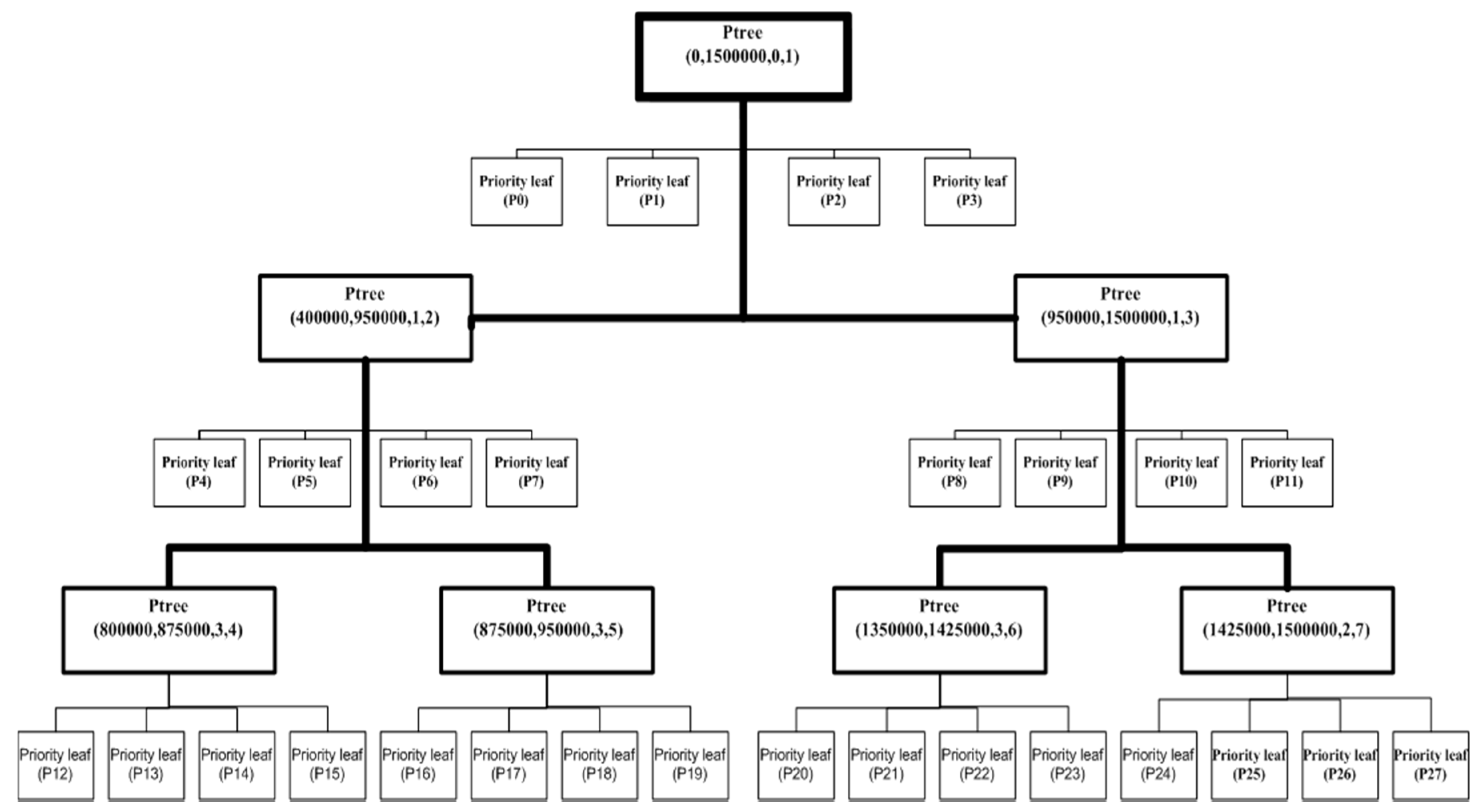
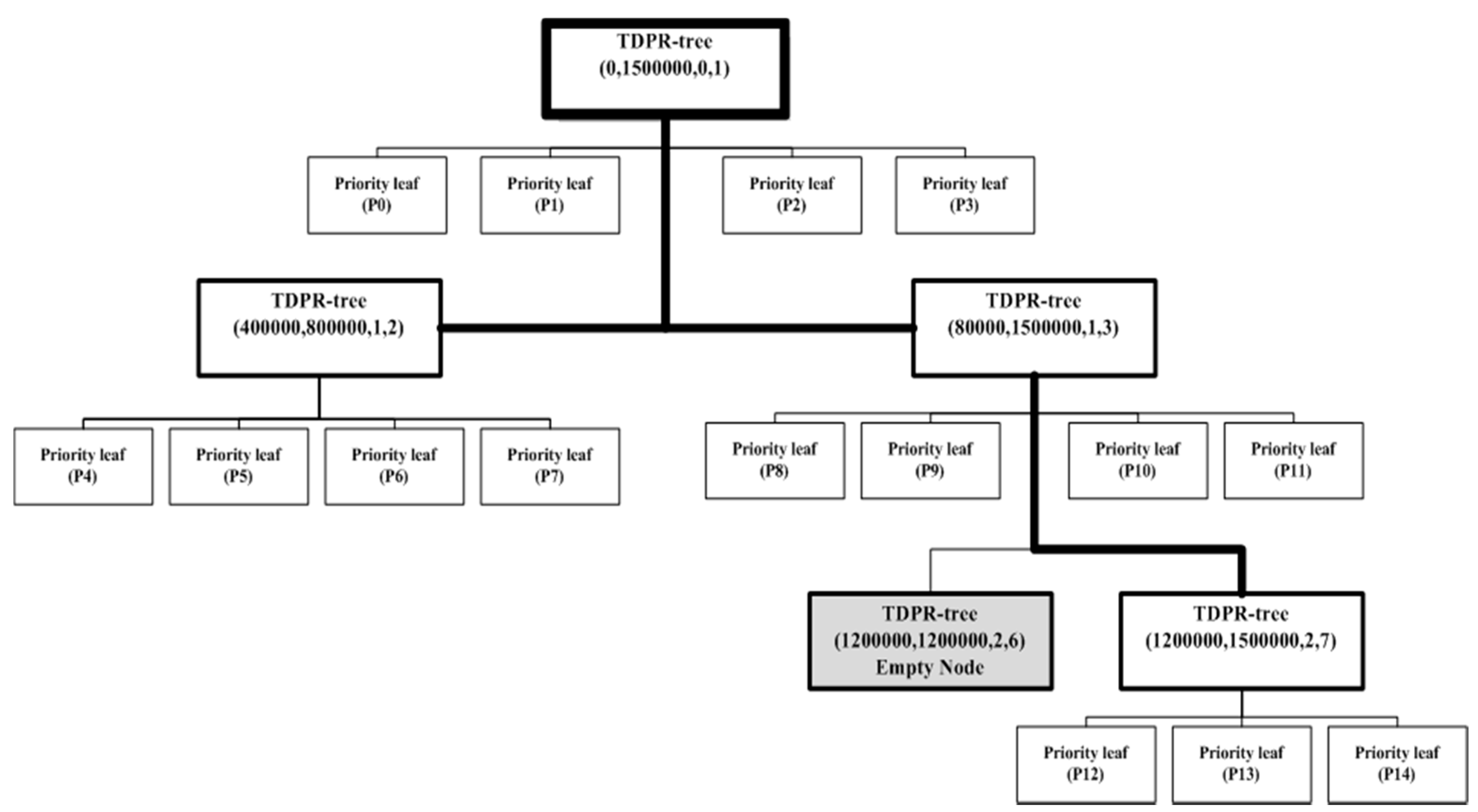
As an example, assuming that a file has 1.5 M records and B—the maximum capacity of the partition—is equal to 100,000 records, the desired number of partitions should be 15 partitions. Figure 2 shows the structure of the traditional PR-Tree of the file using Algorithm 1. It generates 12 partitions with a full capacity (100,000 records) and 16 partitions with 18,750 records each. Therefore, the traditional PR-Tree divides the input file into 28 partitions. Figure 3 shows the structure of the 2DPR-Tree for the same file. It generates 15 partitions at full capacity, achieving 100% space utilization and satisfying the desired number of partitions .
6. Experimentation
6.1. Experimental Setup
All experiments were performed on an EMR Amazon cluster of five ‘m3.xlarge’ nodes, which have a high-frequency 4vCPU Intel Xeon processor, 15 GB of main memory, 2 × 40 GBSSD storage running a Linux operating system, Hadoop2.7.2, and Java 8 [41]. We used synthetic datasets with a uniform distribution in 1 M × 1 M units of area. Each object in the datasets is a rectangle. The synthetic datasets consist of several files with different sizes (1, 2, 4, 8, and 16 GB) that were generated using the SpatialHadoop built-in uniform generator [24]. Additionally, we used real datasets, representing non-uniformly distributed and skewed data, that was extracted from OpenStreetMap, specifically a Buildings data file that had 115 M records of buildings, a Cities data file that had 171 K records of the boundaries of postal code areas (mostly cities), and a Sports data file that had 1.8 M records of sporting areas [12]. Table 3 shows a detailed description of the real datasets.
6.2. Experimental Results
An experimental study comparing the performances of different SpatialHadoop indexing algorithms and the 2DPR-Tree is presented. The experiments show that spatial query processing is very reliant on the size and nature of the dataset, and the indexes demonstrate diverging performance with the alternative dataset types.
Figure 4a shows the graphical representation of the Cities dataset that has been partitioned and indexed into 14 partitions by the 2DPR-Tree using Algorithm 2. Figure 4b–f shows its representation with the other partitioning techniques. It is noted that the spatial locality in the Hilbert and Z-curve techniques is not always well preserved as they generate a high degree of overlap between partitions.
From applying the different partitioning techniques to the uniformly distributed synthetic datasets, an interesting finding is that although all partitioning techniques should partition the input dataset into the same specific number of partitions as mentioned in Section 3, the Quadtree, STR, and STR+ techniques have divided the input datasets into a different number of partitions that are much bigger than desired (Table 4). Table 5 shows that Quadtree divided the Sports, Cities, and Buildings datasets into 25, 34, and 705 partitions, respectively, when the desired number of partitions are 6, 14, and 252 partitions. On the other hand, the 2DPR-Tree, KD-Tree, Z-curve, and Hilbert techniques adhered to the desired number of partitions.
Figure 5 shows the performance measures that assess the indexing time for uniformly distributed synthetic datasets using different techniques. All techniques have approximately the same indexing time for the datasets that are 1, 2, and 4 GB in size. The KD-Tree and Quadtree have the best indexing time for the 8 GB dataset and the 2DPR-Tree has the best indexing time for the 16 GB dataset. For real datasets, Figure 6 shows that 2DPR-Tree has the better indexing time for the datasets of Cities and Buildings.
The range and kNN queries, as presented in the paper by Ahmed Eldawy and Mohamed Mokbel [12], were performed on the partitioned data to quantify and examine the performance of the diverse partitioning strategies. For the range query, the rectangular area A is revolved over arbitrary records from the input dataset. The measure of A is balanced with the end goal that the query area is equal to the selection ratio (σ) multiplied by the total area of the working file, as shown in Equation (1):
where the choice proportion σ ∈ (0, 1] is a parameter we change in our analysis and Area(InMBR) is the region of the MBR of the working file.
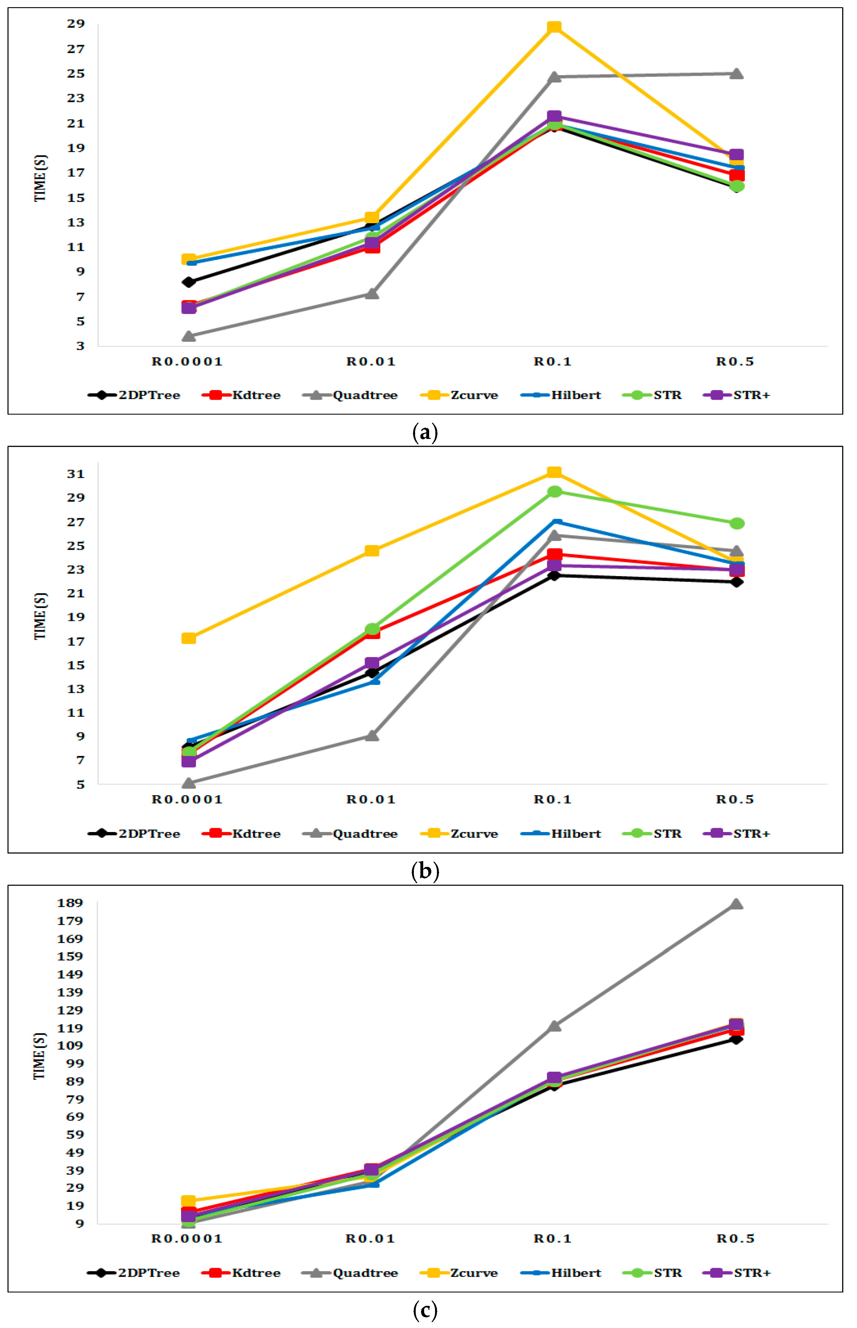
Figure 7a shows the range query processing performance on the indexed synthetic datasets with a query window area equal to 0.01% of the input dataset area. The performance of the 2DPR-Tree and KD-Tree is stable and roughly unchanged through different dataset sizes. On the other hand, the Quadtree, Z-curve, Hilbert, and STR techniques showed varying performances with the change of the input dataset sizes. Figure 7b shows that changing the query window area to 1% of the input dataset area did not have an effect on the performance of the different partitioning techniques for the small size datasets of 1 GB, 2 GB, and 4 GB. For the 8 GB and 16 GB datasets, the range query takes a long time as it must access a greater number of partitions to obtain the query answer. The 2DPR-Tree and KD-Tree take 101 and 103 s, respectively, to answer the range query with 1% query window area on a 16 GB input dataset, which is an excellent result compared to the Quadtree, Z-curve, and Hilbert methods that take 132.5, 127.5, and 112 s, respectively, to answer the same query.
In order to show the effect of changing the size of the query window area on the performance of different partitioning techniques, a range query with a query window area equal to the input dataset area was performed. That query returned all objects in the input dataset and requires the indexing and partitioning technique to access all dataset partitions to obtain the query answer. By comparing results from Figure 7b,c, we find that answering a range query with a query window area equal to the whole input dataset area takes only three times the length of time that it takes to answer a range query with a query window area equal to 1% of the input dataset area. Therefore, the query window area does not have a significant effect on the performance of the range query with different indexing and partitioning techniques. The size of the input dataset, the number of partitions that are generated by the partitioning techniques, and the number of partitions that need to be accessed to get the result have the largest effect on the performance of the range query with different partitioning techniques. As shown in Figure 7b,c, the Quadtree method that divides the 8 GB and 16 GB input datasets into 256 partitions takes much more time to answer the query than the other techniques that divide the 8 GB and 16 GB input datasets into 77,154 partitions.
Figure 8a,b shows the range query processing performance on the Sports and Cities datasets with different query window areas. Quadtree has the best time performance for the range queries with small query window areas equal to 0.01% and 1% of the input dataset area. However, for the range queries with larger query window areas equal to 10% and 50% of the input dataset area, the Quadtree performance rapidly decreased. This is because when the query window area is increased, the number of partitions that is required to be processed to answer the range query is increased, especially for the Quadtree as it partitions the input datasets into a greater number of partitions than the other techniques. On the other hand, the 2DPR-Tree has the best time performance for the range query with query window areas equal to 10% and 50% of the input dataset area, as the 2DPR-Tree divides the input dataset into the desired number of partitions and the spatial proximity of the input shapes is always well preserved. The results shown in Figure 8c confirm our earlier claims as the 2DPR-Tree and the KD-Tree answer the range query with a query window area equal to 50% of the Buildings dataset area in 111 and 120 s, respectively, and Quadtree takes approximately twice the time to answer the same query.
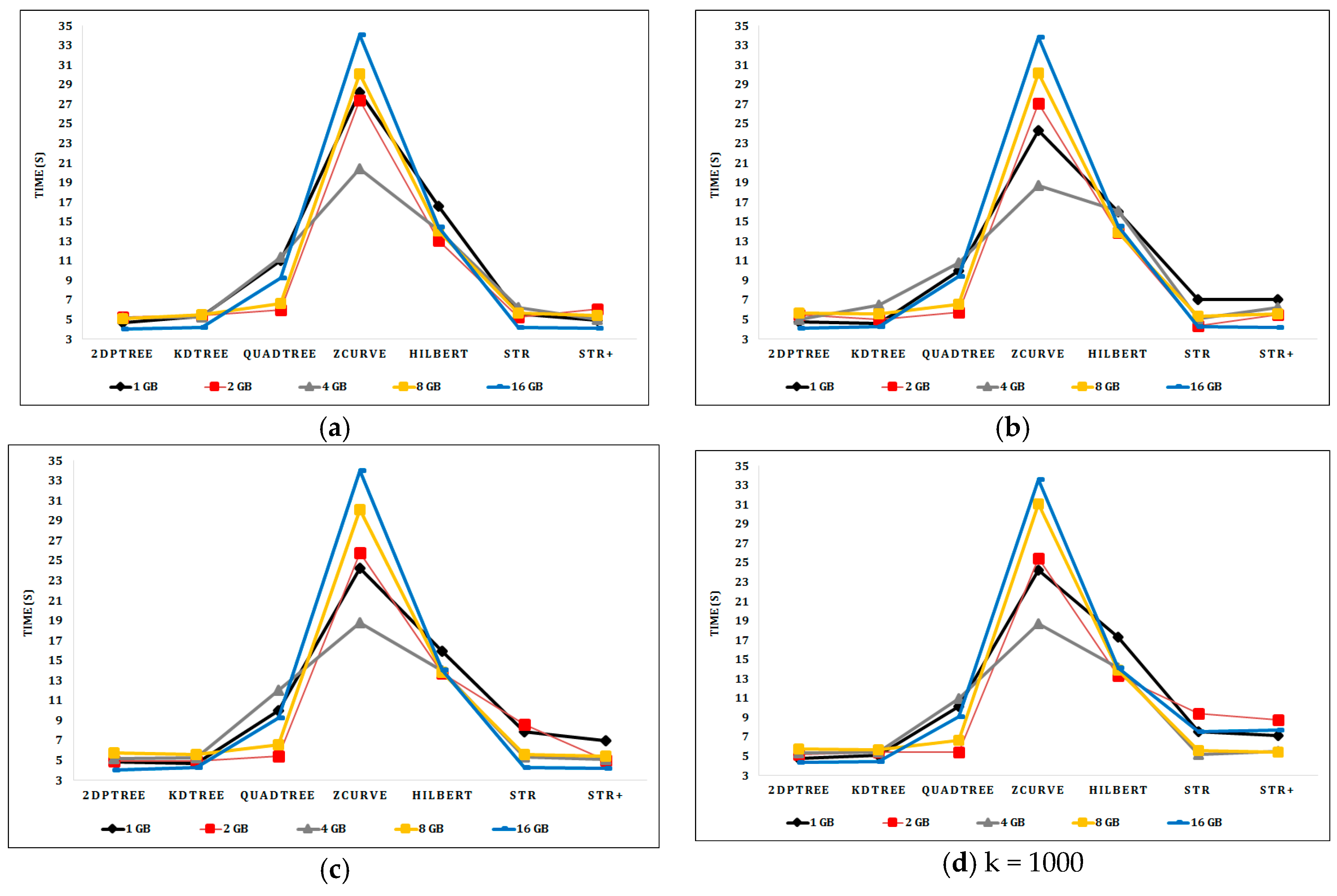
For the kNN query, query locations are arbitrarily chosen from points sampled from the input dataset. Figure 9a–d shows the kNN query performance over the indexed synthetic datasets as the input file size is increased from 1 to 16 GB and k varied from 1–1000. In the uniformly distributed synthetic data, all algorithms have roughly the same performance with different k values. The 2DPR-Tree and KD-Tree techniques, respectively, have the best query execution time for the synthetic datasets.
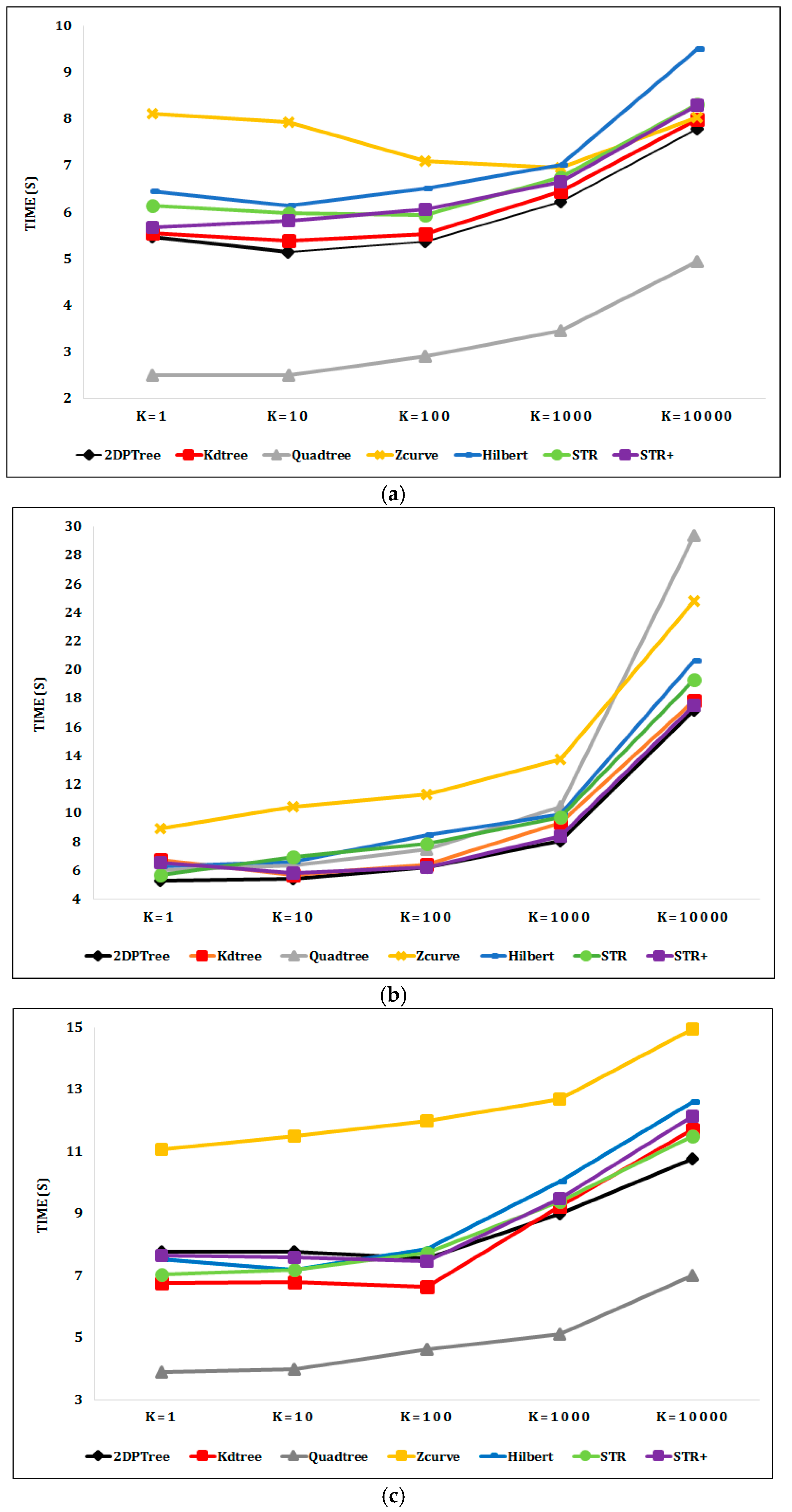
Figure 10a shows the kNN query performance on the Sports dataset as k is varied from 1 to 10,000. Quadtree outperforms the other techniques in performing the kNN queries as it divides the Sports dataset into 25 smaller partitions, in contrast with the other techniques that divide the Sports dataset into six larger partitions. The partition access time of Quadtree is therefore much lower than that of the other techniques, and the kNN query requires a smaller number of partitions to be accessed to get the query result. However, the 2DPR-Tree performs best at the level of techniques that are committed to the desired number of partitions, which is calculated in the initial stage of the partitioning phase and should be fixed for all partitioning techniques. Figure 10b shows the 2DPR-Tree has the best performance for the kNN queries on the Cities dataset with different k values. For the Buildings dataset, Figure 10c shows that Quadtree outperforms the other techniques. However, the KD-Tree has the best kNN query execution time for k equal to 1, 10, and 100 points and the 2DPR-Tree has the best kNN query execution time for k equal to 1000 and 10,000 points, among the techniques that are committed to the desired number of partitions.
7. Conclusions
In this paper, we presented the 2DPR-Tree as a new partitioning technique in SpatialHadoop. An extensive experimental study was performed to compare the proposed 2DPR-Tree with state-of-the-art SpatialHadoop techniques. Various techniques were experimentally evaluated using different types of datasets (synthetic and real) with different distributions (uniformly and non-uniformly distributed data). The Quadtree, STR, and STR+ techniques were not restricted with the desired number of partitions, so they required much more time to build the index. The proposed 2DPR-Tree outperforms other techniques in indexing time for a 16 GB synthetic dataset and for the Cities and Buildings real datasets. For the range query, the performance of the 2DPR-Tree and KD-Tree was stable and roughly unchanged throughout use of the different synthetic datasets. On the other hand, the Quadtree, Z-curve, Hilbert, and STR showed varying performances with the changing of the synthetic dataset sizes. For the real datasets, Quadtree performed best for the range queries with small query window areas equal to 0.01% and 1% of the input dataset area. However, for range queries with larger query window areas equal to 10% and 50% of the input dataset area, the performance of this method rapidly decreased. On the other hand, the 2DPR-Tree performed best for range queries with large query window areas. The 2DPR-Tree and KD-Tree answer the range query with a query window area equal to 50% of the Buildings dataset area in 111 and 120 s, respectively, and Quadtree takes approximately twice the amount of time to answer the same query. For the kNN query, all partitioning techniques have roughly the same performance with different k values for the synthetic datasets. For real datasets, Quadtree outperforms other techniques as it divides the input datasets into a large number of small partitions, in contrast with the other techniques that are restricted to a specific number of larger partitions. Therefore, the partition access time of Quadtree is much lower than that of the other techniques. In addition, the kNN query requires a small number of partitions to be accessed to achieve the result. However, the 2DPR-Tree performs best for the kNN queries with high k values among the techniques that are committed to the desired number of partitions. Therefore, the proposed 2DPR-Tree is significantly better than the other partitioning techniques. As part of our future work, we will develop new multi-dimensional spatial data types on SpatialHadoop, and a new indexing technique for these data types will be developed with the goal of further enhancing query response time and query result accuracy.
Author Contributions
A.E. came up with the original research idea; A.M.R. advised A.E., A.S., and A.A.-F. on the experiment design and paper structure; A.E. and A.S. designed the experiments, deployed the experiment environment, developed the scripts for experiments, and conducted the experiments. Al.M.R. and A.A.-F. analyzed the experiment results; all authors drafted the manuscript; and read and approved the final manuscript.
Acknowledgments
The authors would like to thank the editor and the anonymous reviewers for their systematic reviews, valuable comments and suggestions to improve the quality of the paper.
Conflicts of Interest
The authors declare no conflict of interest.
References
- Cary, A.; Yesha, Y.; Adjouadi, M.; Rishe, N. Leveraging cloud computing in geodatabase management. In Proceedings of the IEEE International Conference on Granular Computing, San Jose, CA, USA, 14–16 August 2010. [Google Scholar]
- Li, Z.; Hu, F.; Schnase, J.L.; Duffy, D.Q.; Lee, T.; Bowen, M.K.; Yang, C. A spatiotemporal indexing approach for efficient processing of big array-based climate data with mapreduce. Int. J. Geogr. Inf. Sci. 2017, 31, 17–35. [Google Scholar] [CrossRef]
- Haynes, D.; Ray, S.; Manson, S. Terra populus: Challenges and opportunities with heterogeneous big spatial data. In Advances in Geocomputation: Geocomputation 2015–the 13th International Conference; Griffith, D.A., Chun, Y., Dean, D.J., Eds.; Springer International Publishing: Cham, Switzerland, 2017; pp. 115–121. [Google Scholar]
- Katzis, K.; Efstathiades, C. Resource management supporting big data for real-time applications in the 5g era. In Advances in Mobile Cloud Computing and Big Data in the 5g Era; Mavromoustakis, C.X., Mastorakis, G., Dobre, C., Eds.; Springer International Publishing: Cham, Switzerland, 2017; pp. 289–307. [Google Scholar]
- White, T. Hadoop: The Definitive Guide; O’Reilly Media: Scbastopol, CA, USA, 2015. [Google Scholar]
- Thusoo, A.; Sarma, J.S.; Jain, N.; Shao, Z.; Chakka, P.; Anthony, S.; Liu, H.; Wyckoff, P.; Murthy, R. Hive: A warehousing solution over a map-reduce framework. Proc. VLDB Endow. 2009, 2, 1626–1629. [Google Scholar] [CrossRef]
- Li, F.; Ooi, B.C.; Ozsu, M.T.; Wu, S. Distributed data management using mapreduce. ACM Comput. 2014, 46, 31–42. [Google Scholar] [CrossRef]
- Doulkeridis, C.; Nrvag, K. A survey of large-scale analytical query processing in mapreduce. VLDB J. 2014, 23, 355–380. [Google Scholar] [CrossRef]
- Eldawy, A.; Li, Y.; Mokbel, M.F.; Janardan, R. Cg_hadoop: Computational geometry in mapreduce. In Proceedings of the 21st ACM SIGSPATIAL International Conference on Advances in Geographic Information Systems, Orlando, FL, USA, 5–8 November 2013; pp. 294–303. [Google Scholar]
- Dean, J.; Ghemawat, S. Mapreduce: Simplified data processing on large clusters. Commun. ACM 2008, 51, 107–113. [Google Scholar] [CrossRef]
- Wang, K. Accelerating spatial data processing with mapreduce. In Proceedings of the 2010 IEEE 16th International Conference on ICPADS, Shanghai, China, 8–10 December 2010. [Google Scholar]
- Eldawy, A.; Mokbel, M.F. Spatialhadoop: A mapreduce framework for spatial data. In Proceedings of the ICDE Conference, Seoul, Korea, 13–17 April 2015; pp. 1352–1363. [Google Scholar]
- Maleki, E.F.; Azadani, M.N.; Ghadiri, N. Performance evaluation of spatialhadoop for big web mapping data. In Proceedings of the 2016 Second International Conference on Web Research (ICWR), Tehran, Iran, 27–28 April 2016; pp. 60–65. [Google Scholar]
- Aly, A.M.; Elmeleegy, H.; Qi, Y.; Aref, W. Kangaroo: Workload-aware processing of range data and range queries in hadoop. In Proceedings of the Ninth ACM International Conference on Web Search and Data Mining, San Francisco, CA, USA, 22–25 February 2016; pp. 397–406. [Google Scholar]
- Zhang, S.; Han, J.; Liu, Z.; Wang, K.; Feng, S. Spatial queries evaluation with mapreduce. In Proceedings of the 2009 Eighth International Conference on Grid and Cooperative Computing, Lanzhou, China, 27–29 August 2009; pp. 287–292. [Google Scholar]
- Ma, Q.; Yang, B.; Qian, W.; Zhou, A. Query processing of massive trajectory data based on mapreduce. In Proceedings of the First International Workshop on Cloud Data Management, Hong Kong, China, 2 November 2009; pp. 9–16. [Google Scholar]
- Akdogan, A.; Demiryurek, U.; Banaei-Kashani, F.; Shahabi, C. Voronoi-based geospatial query processing with mapreduce. In Proceedings of the 2010 IEEE Second International Conference on Cloud Computing Technology and Science, Indianapolis, IN, USA, 30 November–3 December 2010; pp. 9–16. [Google Scholar]
- Nodarakis, N.; Rapti, A.; Sioutas, S.; Tsakalidis, A.K.; Tsolis, D.; Tzimas, G.; Panagis, Y. (a)knn query processing on the cloud: A survey. In Algorithmic Aspects of Cloud Computing: Second International Workshop, Algocloud 2016, Aarhus, Denmark, August 22, 2016, Revised Selected Papers; Sellis, T., Oikonomou, K., Eds.; Springer International Publishing: Cham, Switzerland, 2017; pp. 26–40. [Google Scholar]
- Ray, S.; Simion, B.; Brown, A.D.; Johnson, R. A parallel spatial data analysis infrastructure for the cloud. In Proceedings of the 21st ACM SIGSPATIAL International Conference on Advances in Geographic Information Systems, Orlando, FL, USA, 5–8 November 2013; pp. 284–293. [Google Scholar]
- Ray, S.; Simion, B.; Brown, A.D.; Johnson, R. Skew-resistant parallel in-memory spatial join. In Proceedings of the 26th International Conference on Scientific and Statistical Database Management, Aalborg, Denmark, 30 June–2 July 2014; pp. 1–12. [Google Scholar]
- Vo, H.; Aji, A.; Wang, F. Sato: A spatial data partitioning framework for scalable query processing. In Proceedings of the 22nd ACM SIGSPATIAL International Conference on Advances in Geographic Information Systems, Dallas, TX, USA, 4–7 November 2014; pp. 545–548. [Google Scholar]
- Pertesis, D.; Doulkeridis, C. Efficient skyline query processing in spatialhadoop. Inf. Syst. 2015, 54, 325–335. [Google Scholar] [CrossRef]
- Eldawy, A.; Alarabi, L.; Mokbel, M.F. Spatial partitioning techniques in spatialhadoop. In Proceedings of the International Conference on Very Large Databases, Kohala Coast, HI, USA, 31 August–4 September 2015. [Google Scholar]
- Eldawy, A.; Mokbel, M.F. The ecosystem of spatialhadoop. SIGSPATIAL Spec. 2015, 6, 3–10. [Google Scholar] [CrossRef]
- Randolph, W.; Chandrasekhar Narayanaswaml, F.; Kankanhalll, M.; Sun, D.; Zhou, M.-C.; Yf Wu, P. Uniform Grids: A Technique for Intersection Detection on Serial and Parallel Machines. In In Proceedings of the Auto Carto 9, Baltimore, Maryland, 2–7 April 1989; pp. 100–109. [Google Scholar]
- Singh, H.; Bawa, S. A survey of traditional and mapreduce based spatial query processing approaches. SIGMOD Rec. 2017, 46, 18–29. [Google Scholar] [CrossRef]
- Tan, K.-L.; Ooi, B.C.; Abel, D.J. Exploiting spatial indexes for semijoin-based join processing in distributed spatial databases. IEEE Trans. Knowl. Data Eng. 2000, 12, 920–937. [Google Scholar]
- Zhang, R.; Zhang, C.-T. A brief review: The z-curve theory and its application in genome analysis. Curr. Genom. 2014, 15, 78–94. [Google Scholar] [CrossRef] [PubMed]
- Meng, L.; Huang, C.; Zhao, C.; Lin, Z. An improved hilbert curve for parallel spatial data partitioning. Geo-Spat. Inf. Sci. 2007, 10, 282–286. [Google Scholar] [CrossRef]
- Liao, H.; Han, J.; Fang, J. Multi-dimensional index on hadoop distributed file system. In Proceedings of the 2010 IEEE Fifth International Conference on Networking, Architecture, and Storage, Macau, China, 15–17 July 2010; pp. 240–249. [Google Scholar]
- Guttman, A. R-trees: A dynamic index structure for spatial searching. SIGMOD Rec. 1984, 14, 47–57. [Google Scholar] [CrossRef]
- Beckmann, N.; Kriegel, H.-P.; Schneider, R.; Seeger, B. The r*-tree: An efficient and robust access method for points and rectangles. SIGMOD Rec. 1990, 19, 322–331. [Google Scholar] [CrossRef]
- Leutenegger, S.T.; Lopez, M.A.; Edgington, J. Str: A simple and efficient algorithm for r-tree packing. In Proceedings of the 13th International Conference on Data Engineering, Birmingham, UK, 7–11 April 1997; pp. 497–506. [Google Scholar]
- Giao, B.C.; Anh, D.T. Improving sort-tile-recursive algorithm for r-tree packing in indexing time series. In Proceedings of the the 2015 IEEE RIVF International Conference on Computing & Communication Technologies–Research, Innovation, and Vision for Future (RIVF), Can Tho, Vietnam, 25–28 January 2015; pp. 117–122. [Google Scholar]
- Sellis, T. The r+-tree: A dynamic index for multidimensional objects. In Proceedings of the 13th International Conference on Very Large Data Bases, Brighton, UK, 1–4 September 1987; pp. 507–518. [Google Scholar]
- Bentley, J.L. Multidimensional binary search trees used for associative searching. Commun. ACM 1975, 18, 509–517. [Google Scholar] [CrossRef]
- Olston, C.; Reed, B.; Srivastava, U.; Kumar, R.; Tomkins, A. Pig latin: A not-so-foreign language for data processing. In Proceedings of the 2008 ACM SIGMOD International Conference on Management of Data, Vancouver, BC, Canada, 9–12 June 2008; pp. 1099–1110. [Google Scholar]
- Arge, L.; Berg, M.D.; Haverkort, H.J.; Yi, K. The priority r-tree: A practically efficient and worst-case optimal r-tree. ACM Trans. Algorithms 2008, 4, 9. [Google Scholar] [CrossRef]
- Agarwal, P.K.; Berg, M.D.; Gudmundsson, J.; Hammar, M.; Haverkort, H.J. Box-trees and r-trees with near-optimal query time. Discre. Comput. Geom. 2002, 28, 291–312. [Google Scholar] [CrossRef]
- Davies, J. Implementing the Pseudo Priority r-Tree (pr-tree), a Toy Implementation for Calculating Nearest Neighbour on Points in the x-y Plane. Available online: http://juliusdavies.ca/uvic/report.html (accessed on 18 August 2017).
- Amazon. Amazon ec2. Available online: http://aws.amazon.com/ec2/ (accessed on 10 January 2018).
Figure 1.
SpatialHadoop system architecture [12].
Figure 1.
SpatialHadoop system architecture [12].
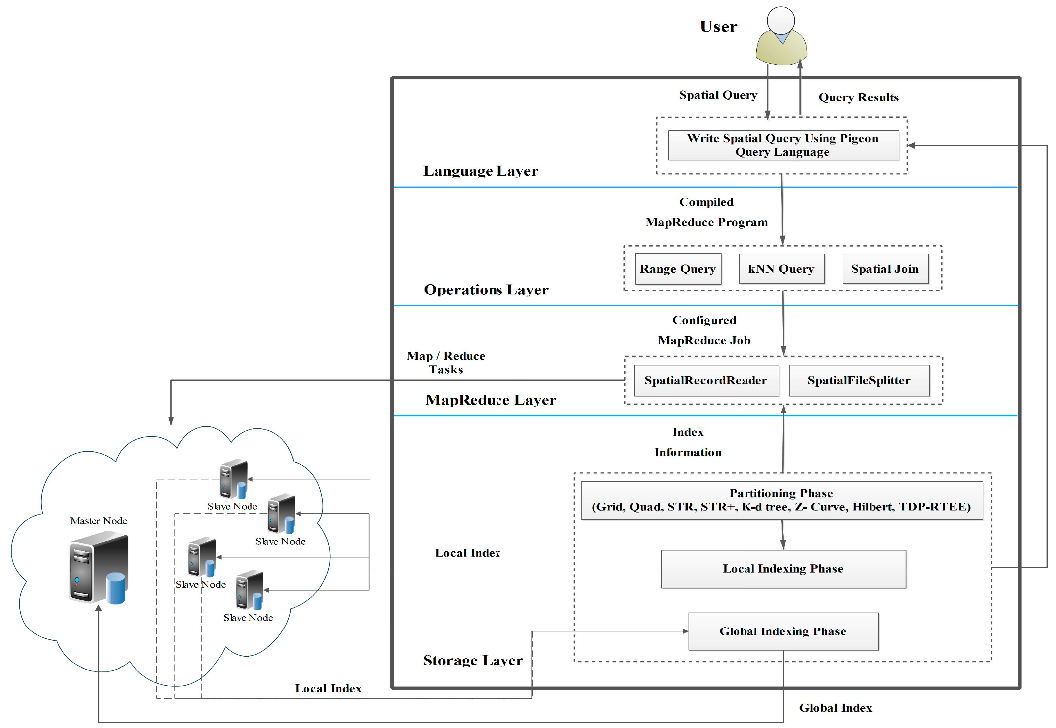
Figure 2.
PR-Tree structure for a file with a 1.5 M rectangle.

Figure 3.
2DPR-Tree structure for a file with a 1.5 M rectangle.

Figure 4.
The Cities dataset indexed with different SpatialHadoop indexing techniques: (a) Cities indexed with the 2DPR-Tree; (b) Cities indexed with the KD-Tree; (c) Cities indexed with the Quadtree; (d) Cities indexed with the Hilbert-Curve; (e) Cities indexed with the Z-Curve; (f) Cities indexed with the STR and STR+.

Figure 5.
Indexing time for the synthetic datasets.
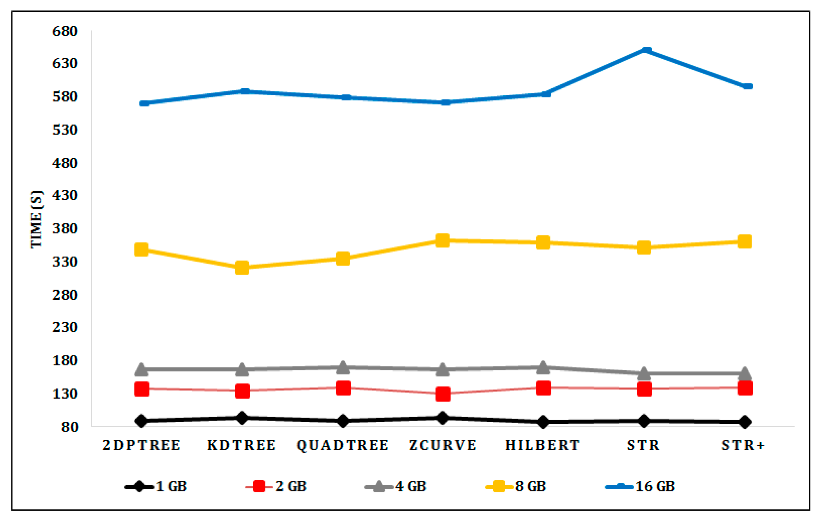
Figure 6.
Indexing time for the real datasets (Sports, Cities, and Buildings).
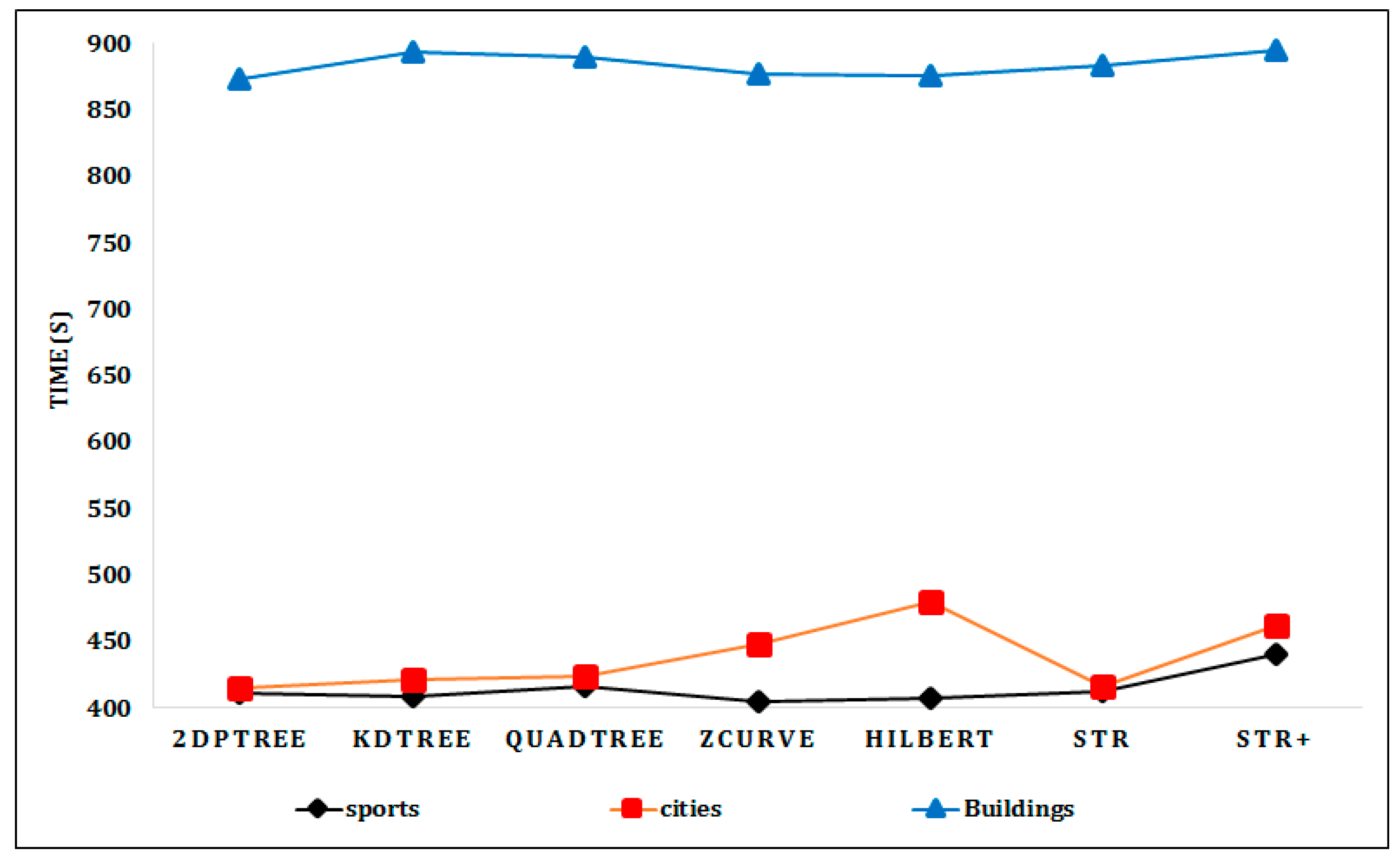
Figure 7.
Range query execution time on indexed synthetic datasets: (a) Range query with a 0.0001 query window area; (b) range query with a 0.01 query window area; (c) range query with a query window area equal to the file area.
Figure 7.
Range query execution time on indexed synthetic datasets: (a) Range query with a 0.0001 query window area; (b) range query with a 0.01 query window area; (c) range query with a query window area equal to the file area.
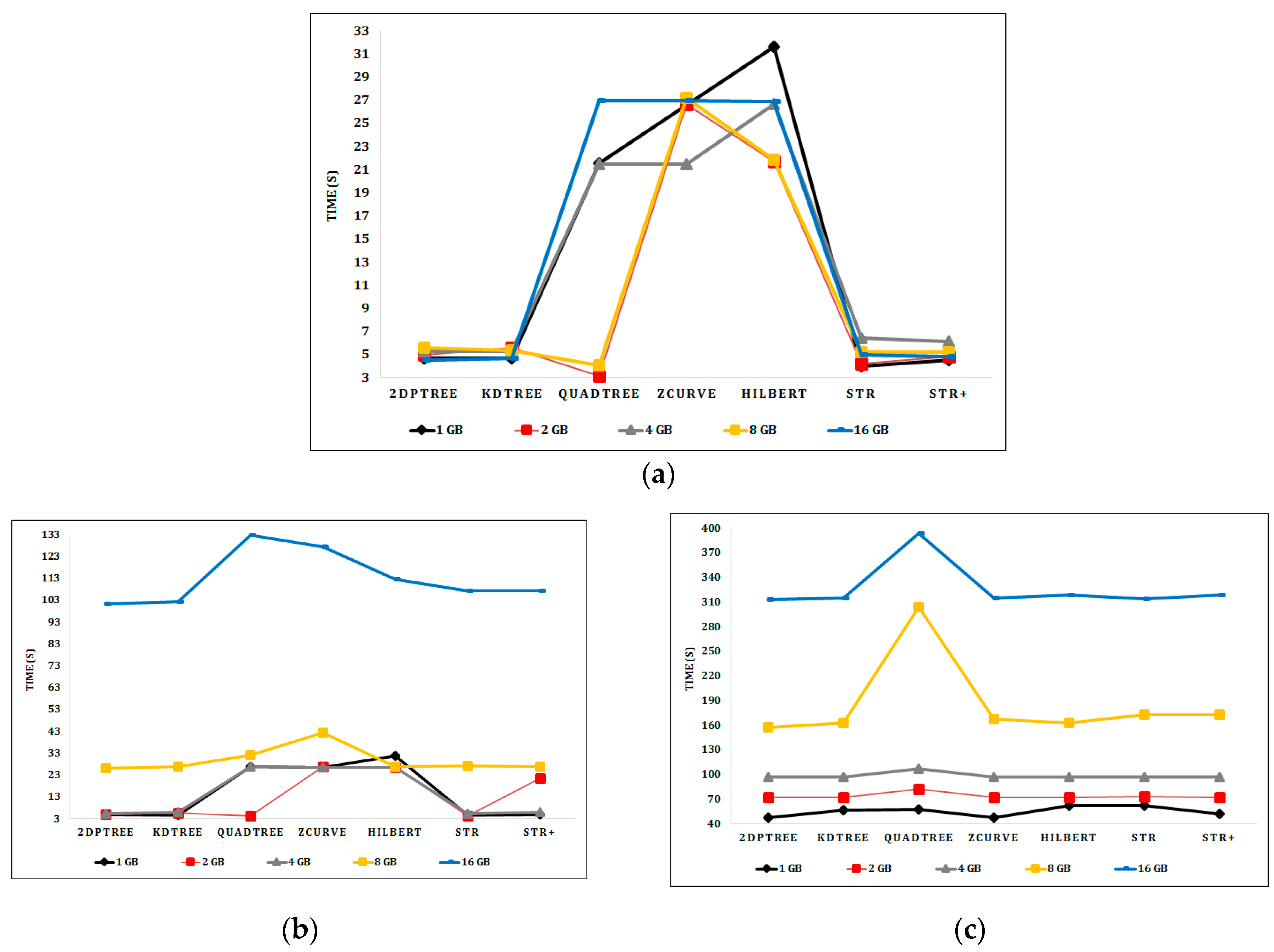
Figure 8.
Range query execution time for indexed real datasets: (a) Query window area equal to 0.01%, 1%, 10%, and 50% of the Sports dataset area; (b) query window area equal to 0.01%, 1%, 10%, and 50% of the Cities dataset area; (c) query window area equal to 0.01%, 1%, 10%, and 50% of the Buildings dataset area.

Figure 9.
kNN query execution time for indexed synthetic datasets: (a) With k = 1; (b) with k = 10; (c) with k = 100; (d) with k = 1000.
Figure 9.
kNN query execution time for indexed synthetic datasets: (a) With k = 1; (b) with k = 10; (c) with k = 100; (d) with k = 1000.

Figure 10.
kNN query execution times for indexed real datasets: (a) kNN on the Sports dataset with k equal to 1, 10, 100, 1000, and 10,000 points; (b) kNN on the Cities dataset with k equal to 1, 10, 100, 1000, and 10,000 points; (c) kNN on the Buildings dataset with k equal to 1, 10, 100, 1000, and 10,000 points.


Table 1.
A general classification of SpatialHadoop partitioning techniques.
| Dimension | Category | Grid | Quad Tree | Z Curve | Hilbert Curve | STR | STR+ | KD-Tree | 2DPR-Tree |
|---|---|---|---|---|---|---|---|---|---|
| Partition Boundary | overlapping | √ | √ | √ | √ | ||||
| non-overlapping | √ | √ | √ | √ | |||||
| Search Strategy | top-down | N/A | N/A | √ | √ | ||||
| bottom-up | N/A | N/A | √ | √ | √ | √ | |||
| Split Criterion | space-oriented | √ | √ | ||||||
| space-filling curve (SFC)-oriented | √ | √ | |||||||
| data-oriented | √ | √ | √ | √ |
Table 2.
Description of symbols that are used in the algorithms.
| Symbol | Description |
|---|---|
| S | Set of rectangles in the working file |
| N | Rectangles number in S. |
| np | The number of shapes/points to be indexed |
| PN | Partition number calculated by dividing the size of working file by the file block size as each partition should fit into only one file block |
| B | Number of shapes/points assigned for each partition or file block calculated as np/PN |
| Set of 4D points (a point for each rectangle in S) | |
| Set of 2D points (a 2D point for each rectangle in S) | |
| RN | Initial node (root) with start index = 0 and end index = S*. length and depth = 0 |
| µ | Median (the divider that splits the rest of the points into two almost equal sized subsets) |
Table 3.
Real spatial datasets.
| Name | Data Size | Records No. | Average Record Size | Description |
|---|---|---|---|---|
| Buildings | 28.2 GB | 115 M | 263 bytes | Boundaries of all buildings |
| Cities | 1.4 GB | 171 K | 8.585 KB | Boundaries of postal code areas (mostly cities) |
| Sports | 590 MB | 1.8 M | 343 bytes | Boundaries of sporting areas |
Table 4.
Partition number generated by indexing techniques in the synthetic datasets.
| File Size (GB) | Partitions NO | ||||
|---|---|---|---|---|---|
| 1 GB | 2 GB | 4 GB | 8 GB | 16 GB | |
| 2DPR-Tree | 10 | 20 | 39 | 77 | 154 |
| KD-Tree | 10 | 20 | 39 | 77 | 154 |
| Quadtree | 16 | 64 | 64 | 256 | 256 |
| Z-curve | 10 | 20 | 39 | 77 | 154 |
| Hilbert | 10 | 20 | 39 | 77 | 154 |
| STR & STR+ | 12 | 20 | 42 | 81 | 156 |
Table 5.
Partition number generated by indexing techniques in the real datasets.
| Real Dataset | Partitions NO | ||
|---|---|---|---|
| Sports | Cities | Buildings | |
| 2DPR-Tree | 6 | 14 | 252 |
| KD-Tree | 6 | 14 | 252 |
| Quadtree | 25 | 34 | 705 |
| Z-curve | 6 | 14 | 252 |
| Hilbert | 6 | 14 | 252 |
| STR & STR+ | 6 | 18 | 252 |
© 2018 by the authors. Licensee MDPI, Basel, Switzerland. This article is an open access article distributed under the terms and conditions of the Creative Commons Attribution (CC BY) license (http://creativecommons.org/licenses/by/4.0/).
Share and Cite
MDPI and ACS Style
Elashry, A.; Shehab, A.; Riad, A.M.; Aboul-Fotouh, A. 2DPR-Tree: Two-Dimensional Priority R-Tree Algorithm for Spatial Partitioning in SpatialHadoop. ISPRS Int. J. Geo-Inf. 2018, 7, 179. https://doi.org/10.3390/ijgi7050179
AMA Style
Elashry A, Shehab A, Riad AM, Aboul-Fotouh A. 2DPR-Tree: Two-Dimensional Priority R-Tree Algorithm for Spatial Partitioning in SpatialHadoop. ISPRS International Journal of Geo-Information. 2018; 7(5):179. https://doi.org/10.3390/ijgi7050179
Chicago/Turabian StyleElashry, Ahmed, Abdulaziz Shehab, Alaa M. Riad, and Ahmed Aboul-Fotouh. 2018. "2DPR-Tree: Two-Dimensional Priority R-Tree Algorithm for Spatial Partitioning in SpatialHadoop" ISPRS International Journal of Geo-Information 7, no. 5: 179. https://doi.org/10.3390/ijgi7050179
Note that from the first issue of 2016, this journal uses article numbers instead of page numbers. See further details here.