Article

Evaluating the Open Source Data Containers for Handling Big Geospatial Raster Data

1
NSF Spatiotemporal Innovation Center and Department of Geography and GeoInformation Science, George Mason University, Fairfax, VA 22030, USA
2
NASA Goddard Space Flight Center, Greenbelt, MD 20771, USA
*
Author to whom correspondence should be addressed.
ISPRS Int. J. Geo-Inf. 2018, 7(4), 144; https://doi.org/10.3390/ijgi7040144
Submission received: 26 February 2018 / Revised: 5 April 2018 / Accepted: 5 April 2018 / Published: 7 April 2018

Abstract

:
Big geospatial raster data pose a grand challenge to data management technologies for effective big data query and processing. To address these challenges, various big data container solutions have been developed or enhanced to facilitate data storage, retrieval, and analysis. Data containers were also developed or enhanced to handle geospatial data. For example, Rasdaman was developed to handle raster data and GeoSpark/SpatialHadoop were enhanced from Spark/Hadoop to handle vector data. However, there are few studies to systematically compare and evaluate the features and performances of these popular data containers. This paper provides a comprehensive evaluation of six popular data containers (i.e., Rasdaman, SciDB, Spark, ClimateSpark, Hive, and MongoDB) for handling multi-dimensional, array-based geospatial raster datasets. Their architectures, technologies, capabilities, and performance are compared and evaluated from two perspectives: (a) system design and architecture (distributed architecture, logical data model, physical data model, and data operations); and (b) practical use experience and performance (data preprocessing, data uploading, query speed, and resource consumption). Four major conclusions are offered: (1) no data containers, except ClimateSpark, have good support for the HDF data format used in this paper, requiring time- and resource-consuming data preprocessing to load data; (2) SciDB, Rasdaman, and MongoDB handle small/mediate volumes of data query well, whereas Spark and ClimateSpark can handle large volumes of data with stable resource consumption; (3) SciDB and Rasdaman provide mature array-based data operation and analytical functions, while the others lack these functions for users; and (4) SciDB, Spark, and Hive have better support of user defined functions (UDFs) to extend the system capability.

1. Introduction

Over the past decade geospatial raster data have grown exponentially due to the recent advancements in data acquisition technology and high-precision simulations of geophysical phenomena [1,2]. For example, the Landsat archive holds over five million images of the Earth’s surface in 5 PB [3]. The National Aeronautics and Space Administration (NASA) will host about 350 petabytes of climate data by 2030 [4].
The big volume with the computational intensive nature of multi-dimensional raster data pose grand challenges to the storage technologies for effective big data management [5,6]. Meanwhile, the special features of geospatial raster data (e.g., varied formats, different coordinate systems, and various resolutions) bring additional challenges [7]. For example, when storing and accessing geospatial data, the coordinate information needs to be kept in the system for spatial queries, and the system needs to transform the coordinate systems for the data from different resources. To address these challenges for massive Earth observation and simulation data management and processing, various big data container software/solutions/infrastructures have been developed by geoscience communities and other communities to facilitate the storage, retrieval, and analysis of big data. Such open source data containers include Spark, ClimateSpark, Hive, Rasdaman, SciDB, and MongoDB [8,9,10,11,12]. Spark (2014, Apache v2.0 License) and Hive (2014, Apache v2.0 License) are two of the most popular Apache projects with active code contribution from the open source community and industry companies. ClimateSpark (2015) is a research project in collaboration between the NSF Spatiotemporal Innovation Center (STC) and NASA Center for Climate Simulation (NCCS). Both Rasdaman (1989, GNU LGPL for client libraries, GNU GPL v3.0 for servers) and SciDB (2008, AGPL v3.0) were incubated in universities and then start-up companies were built behind the projects. They have both the community edition and the enterprise edition with more functionality and support. MongoDB (2007, various licenses with GNU AGPL v3.0 and Apache License for no cost) is mainly developed by MongoDB Inc. and shifted to an open source development model in 2009. These containers optimize their performance from different aspects, such as data organization modeling, indexing, and data pipelines. However, there are few studies to comprehensively evaluate these technologies and tools in supporting the archive, discovery, access, and processing of the large volume of geospatial raster data. This paper investigates and systematically compares the features and performances of these six popular data containers by using different types of spatial and temporal queries for the geospatial datasets stored in common scientific data formats (e.g., NetCDF and HDF). The runtime and computing resources (e.g., CPU, memory, hard drive, and network) consumption are assessed for their performance evaluation and analysis.
Section 2 reviews related research on geospatial data management and processing, while Section 3 compares the features of the selected data containers for geospatial data. Section 4 evaluates the capabilities of different data containers in geospatial data storing, managing, and querying, and Section 5 summarizes this study and discusses future work.

2. Related Work

There are different data containers used to manage big geospatial raster data. The data containers can be categorized into relational database-management system (RDBMS), Array-based DBMS, and NoSQL DBMS [13].

2.1. Relational DBMS

A relational database management system (RDBMS) is built on the relational model, which is not suitable for multi-dimensional data (e.g., scientific raster data, spatial or temporal ordering data). However, since RDSMSs have been widely used, researchers developed fixes to its shortcoming of storing spatial data. For example, PostGIS is a free spatial database extension for PostgreSQL, allowing users to create location-aware queries in SQL format and build their own backend for mapping purposes, raster analyses, and routing applications. Davies et al. (2009) successfully implemented a use case using PostGIS extension to store MODIS fire archive [14]. The utilization of MySQL as the backend to manage large raster data for WebGIS is another application of RDBMSs for spatial data [15,16,17,18]. Scalability is another indicator measuring how a database supports big data [19,20]. RDBMSs can scale up with expensive hardware, but cannot work well with commodity hardware in parallel [21]. To overcome this problem, The Apache Hadoop project develops open-source software to allow the distributed processing of large datasets to work on clusters of commodity computers using simple programming models (http://hadoop.apache.org/). As two of the most popular data containers in the Apache Hadoop ecosystem, Hive and Spark have been used to process geospatial data [11,22]. For example, SciHive extends Hive to implement a scalable, array-based query system to process raw array datasets in parallel with a SQL-like query language [23]. Hadoop-GIS integrates global partition indexing and customizable local spatial indexing techniques into Hive to improve the efficiency of spatial data query on Hive [24]. SciSpark utilizes Spark to develop a scalable scientific processing platform that makes interactive computation and exploration of large volume of raster data [25]. To improve the query performance, Hu et al. (2017) developed a multi-dimensional index to enable Spark to natively support the array-based dataset stored in HDFS. Although the previously mentioned frameworks (e.g., SciHive and SciSpark) achieve scalability, they are not as mature as the traditional RDBMS in terms of system stability, usability, and maintenance [25,26]. For example, Spark’s reliance on the JVM with its greedy usage of memory introduces significant source of latency and impact the cluster’s performance and stability [25].

2.2. Array-Based DBMS

Since the traditional RDBMSs cannot efficiently handle the intrinsically ordered raster data (e.g., satellite images and climate simulation data), Array DBMSs have become a popular area of research for big scientific data management [13,26]. The PICDMS is one of the pioneering Array DBMSs to process image datasets with grid-based database structure [27]. Another pioneering Array DBMS, Rasdaman (“raster data manager”), has a 24-year history and has matured implementation on storage layout, query language, performance optimization, and query evaluation [26]. With the development of GIScience research, more libraries and software (e.g., PostGIS Raster, Oracle generator, ESRI ArcSDE, and SpatiaLite) support array-based datasets. To ease the operation for array datasets, SciQL, an array extension to the column-store MonetDB system, initially designed the SQL-based declarative query language for scientific applications to bridge the gap between the needs of big array data processing and the current DBMS technologies [28]. It seamlessly integrates the array-, set-, and sequence-interpretations by extending the value-based grouping of SQL:2003 with structural grouping [22]. Another new open-source data management system, SciDB, has been developed primarily for the scientific domains involving very large (petabyte) scale array data, such as astronomy, remote sensing, climate modeling, and bio-science information. It supports nested-array data model, science-specific operations, uncertainty, lineage, and named versions [11,29]. User-defined functions provide the users with the flexible capabilities to implement their own array functions for their specific projects. For example, EarthDB utilized SciDB’s support for user-defined functions to implement complex analyses for MODIS data [30].

2.3. NoSQL DBMS

NoSQL (Not Only SQL) refers to the databases built for providing higher performance, elastic scalability, and flexible data modeling. The widely-acknowledged NoSQL database categories are key-value, document, column, and graph, and each has a distinct set of characteristics while all store large volumes of semi-structured or unstructured data with high Read/Write throughput [31]. Aniceto et al. (2014) presented a key-value based NoSQL database (Cassandra) approach to treat genomic data, which involves large volume of data insertion and deletion [32]. They evaluated both persistency and I/O operations with real data and found performance gain compared to the relational database system. However, key-value databases (e.g., Cassandra) provide limited functionality beyond key-value storage and have no support for relationships. Other representative key-value systems include Memcached, Aerospike, Redis, Riak, Kyoto Cabinet, Amazon DynamoDB, and CouchDB. A document-based NoSQL database such as MongoDB is used for managing geospatial data more effectively than key-value database, because geospatial data inside the document database can be retrieved using more flexible queries than key-value based database, and many document databases support geospatial data natively, for example, through GeoJSON format. In addition, proximity queries can be efficiently implemented using document database [31]. Using MongoDB to store and access climate satellite data, Ameri et al. (2014) compared the results with a SQL database (MySQL) [33]. The performance was improved up to a factor of 46 using 11 threads on a 12-core system. However, relationships and joins are not supported as in relational databases, and such systems lack native support for multidimensional data. Other document databases include Couchbase, RavenDB, and FatDB. For the column-based NoSQL databases, the queries are limited to keys and, in many cases, do not have a way to query by column or value, requiring a mapping layer to handle highly connected geospatial data, which is not efficient [31]. Han and Stroulia (2013) demonstrated a data model of stored location data based on column database (HBase) [34]. Although it does not have clear advantages regarding query response time, it scales well and supports efficient performance for range and k-nearest neighbor queries. Other systems in this category include Google BigTable, Cloudata, and Cassandra (also a key-value database).

2.4. Review Summary

There are a few studies that summarize and analyze the above-mentioned data containers [6,13,35]. For example, Rusu and Cheng (2013) provided a guide for past, present, and future research in array processing from the aspects of array storage, array query, and real systems for array processing, but no benchmarking result is provided to measure the performance of different data containers [13]. Merticariu et al. (2015) presented a systematic benchmark of the array-based DBMS on the storage access components, but they did not evaluate NoSQL and Hadoop-based systems [24]. This paper selects six of the above-mentioned data containers (Rasdaman, SciDB, MongoDB, Spark, Hive, and ClimateSpark) for evaluation by considering their popularity and technical features. They cover the mainstream database types. Rasdaman and SciDB are representatives of array-based databases; MongoDB is a classic No-SQL database with high scalability and popular community; Spark and Hive are two of the most popular data warehouses built on top of Hadoop for large-scale data query and analytics; and ClimateSpark develops a multi-dimensional indexing strategy to enable Spark to natively support some array-based datasets (e.g., HDF and NetCDF). Their architectures, technologies, capabilities, and performances are compared and evaluated using the real geospatial raster data, from two perspectives: (a) system design and architecture (distributed architecture, logical data model, physical data model, and data operations); and (b) practical usage experience and performance (data preprocessing, data uploading, query speed, and resource consumption).

3. Data Container Comparison

The six containers (Spark, ClimateSpark, Hive, Rasdaman, SciDB, and MongoDB) are compared for their handling of geospatial data from the perspective of architecture, logical data model, physical data model, and data operations. Among the six compared, Rasdaman was developed by the geoscience community and ClimateSpark is enhanced from Spark for geoscience community.

3.1. Distributed Architecture

All data containers support the standalone and distributed deployment fashion. Distributed architecture is required for handling big geospatial data. In distributed architecture data containers consist of client node, master node, and worker node (Figure 1). The client node is for user interaction of query input and results retrieval. The master node translates queries into tasks and coordinates the worker nodes to conduct the tasks in parallel. The worker nodes receive the assigned tasks from the master node, extract and analyze the specified data, and return them to the master node. Different containers adopt different design theories and techniques to implement the system. The layout of the specific terminologies for each data container uses for client node, master node, and worker/data node is provided (Table 1).

3.1.1. Spark, ClimateSpark, and Hive on YARN and HDFS

Spark utilizes YARN to manage the computing resources and HDFS to support distributed data storage (Figure 2). Each work node launches a NodeManager for computing resource management, scheduling, and monitoring but also serves as a data node for HDFS to achieve high data locality. Different from other containers, the Spark cluster enables users to specify the computing resource requirement when submitting the Spark jobs. ClimateSpark is deployed on the top of Spark cluster with the similar workflow but customized with spatiotemporal index for array-based data to improve query performance.
Hive is built on top of Hadoop for querying and analyzing data stored in various databases and file systems compatible with Hadoop using a declarative query language (HiveQL) (Figure 3). Based on the architecture of Yarn and HDFS, it automatically translates SQL queries to MapReduce jobs by its compiler (including parser, semantic analyzer, logical plan generator, and query plan generator), and executes them over distributed data. The master node (HiveServer2) communicates with MetastoreDB to inventory statistics and schema and then compiles queries from clients to generate query executions, which includes a series of map-reduce serializable tasks. These plans are submitted to YARN and run in parallel as MapReduce tasks. A Tez Application Master (AM) monitors the queries while they are running.
As the distributed file system for Spark and Hive, HDFS (http://hadoop.apache.org/docs/current/hadoop-project-dist/hadoop-hdfs/HdfsDesign.html) is highly fault-tolerant and can be deployed on low-cost hardware, while still providing reliable and high throughput access to data stored accross the cluster. It can automatically detect hardware failure and recover lost data from duplications.

3.1.2. Rasdaman

The master node in Rasdaman (Figure 4) is called Rasdaman host, which serves as the central Rasdaman request dispatcher and controls all server processes. The Rasdaman manager accepts client requests and assigns the server processes to these requests. The server process resolves the assigned requests and then generates calls to the relational server on the database host. According to the calls, the relational server retrieves the specified data from a relational database store. The retrieved data will be sent back to the client node via the network.

3.1.3. SciDB

The master node (coordinator node) of SciDB (Figure 5) serves as the build host to automatically install SciDB across the cluster and host the PostgreSQL server managing the SciDB system catalog. To handle petabyte data, SciDB uses a shared nothing engine, meaning each worker node talks to locally attached storage only for query processing. When an external application connects to SciDB, it connects to one of the nodes in the cluster, but all nodes in the SciDB cluster participate in query execution and data storage. Data are equally distributed in each SciDB node, inclusive of the master node.

3.1.4. MongoDB

Compared with other containers, MongoDB requires an extra Config server (Figure 6) to store the metadata for the shard distribution information (e.g., how the chunks spread among the shards) [36,37]. The master node (Mongos node) caches metadata (e.g., routing table and shard list) from the Config servers and acts as a query router to assign client operations to the appropriate shard node and return results to the client. Data are stored in the worker nodes (shard nodes), and each shard node contains a database portion. When inserting data in a database, the data are uploaded to a random shard server as the primary node, while chunking service distributes data chunks to the rest shards in the cluster.

3.2. Logical Data Model

3.2.1. Array-Based Data Model

The array-based data model is the fundamental data structure in Rasdaman, SciDB, and ClimateSpark to organize datasets (Table 2). An array is a set of elements sorted in multi-dimensional space, and these dimensions are flexible during its definition to allow dynamic growth and reduction over their lifecycle. Each cell/element along the dimensions contains a single or composite value, but all cells share the same structure, and the value position is calculated from the index.
However, there are differences in supporting projections and data types as follows:
  • In Rasdaman, the index of each dimension can only be integer and does not support a geographic coordinate projection. Each cell of the array is defined as the base and composite data types, including nested structures. Arrays are grouped into collections, and collections form the basis for array handling just as tables do in relational database technology.
  • The array in SciDB is specified by dimensions and attributes of the array and supports the geographic coordinate systems. Each dimension consists of a name, a range, a chunk size, and a chunk overlap. The sorted list of dimensions defines the array’s shape, and the cell in the array is a single value or a composition of multiple attributes.
  • ClimateSpark support HDF and NetCDF natively as the default data format. HDF/NetCDF (e.g., HDF4, HDF5, NetCDF 4) is a set of machine-independent data formats to create, access, and share multi-dimensional array-based data. ClimateSpark leverages the array data model in HDF and NetCDF to abstract the array-based raster data. The geo-referencing coordinate system in HDF/NetCDF is supported to identify the coordinates of the data arrays. Variables share dimensions and attributes with each other. The related variables can be collected as a group includes variables, shared attributes, and nested Groups.

3.2.2. Relational Data Model

Spark and Hive use their SQL engine to process geospatial data, so the relation data model represents the geospatial data at the logical level. A relational data model is treated as an array without dimensions but with attributes because the relation table only supports two-dimensional structure. The loss of dimensions requires using dimension attributes to form a key in the corresponding relation. Compared with the array-based model, one views the relational data model as a process that decomposes the array into a set of points with coordinate indices, and store each point as a record in a table.

3.2.3. Key-Value Data Model

MongoDB utilizes the document-oriented data model to store data as collections in documents [38]. Different from RDBMS, there is no fixed schema in MongoDB. MongoDB documents consist of key-value pairs in JavaScript Object Notation (JSON) format, which can be accessed as an object by an object-oriented language [33]. The MongoDB approach begins by identifying the demand queries and then structures the data model to best support these queries [39]. For array-based data, they are mapped into basic tables and then broken down into rows into documents to be stored in MongoDB. The rows of tables are stored as embedded documents or values, and documents have fields with values as arrays. The unique key or ID of each document is generated automatically, however, an additional key or hashed key needs to be generated manually to sharding databases. Inside each document, data are stored as key-value format, where the field names are the keys, and the field content hold corresponding values. There is no fixed schema, which means the fields for each document are not required to be identical among the collections inside the database. The maximum document size is 16 megabytes which helps to ensure the performance when caching the files in memory.
Table 3 illustrates how the array-based datasets are represented in the above three logical data models.

3.3. Physical Data Model

The data containers partition the datasets into small pieces and store them in their own specially designed physical data models to obtain the high query performance and scalability. Table 4 summarize the features of the physical data models of Spark, ClimateSpark, Hive, Rasdaman, SciDB, and MongoDB.

3.3.1. Rasdaman, SciDB, and ClimateSpark

Rasdaman, SciDB, and ClimateSpark use arrays to represent data, but the default array size is usually too large to fit entirely in memory, and the entire array is required to be read whenever an element is queried. Thus, the array is often partitioned into smaller chunks as a basic I/O unit organized on disk, like the page for file systems and the block for relational databases [13], and the chunking structure is invisible to the query client. With the chunking strategy the query process is more efficient since only the involved chunks need to be read instead of the entire array.
Although Rasdaman, SciDB, and ClimateSpark support chunking storage, there are differences when storing data. Rasdaman offers an array storage layout language in its query language to enable users to control the important physical tuning parameter (e.g., chunk size and chunk scheme). The chunk schemes include regular, aligned, directional, and area of interest chunking. The regular chunking method is to equally split array-based datasets into multiple chunks with same dimension size and no overlapping. After users set the chunking parameters, Rasdaman automatically partitions the input data to chunks in the data loading process and stores them with the metadata in local database. Rasdaman also supports different indices for different chunking schemes. Both R+ tree and directory index work with all chunking schemes, whereas the regular computed index only works with regular tiling but is faster than the other indexes.
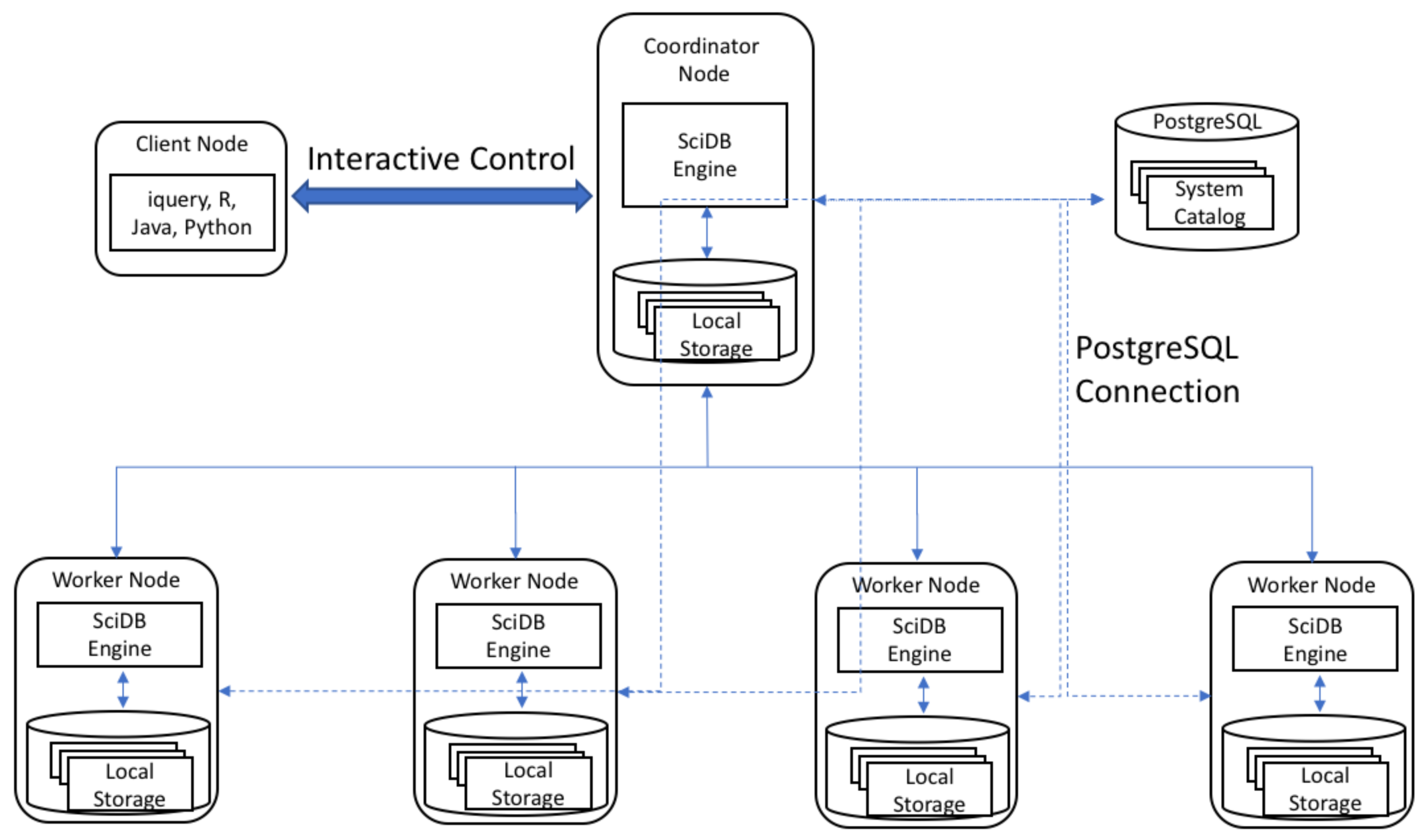
Data stored in SciDB uses a SciDB-specific binary format. The SciDB version (15.12) adopted in this paper utilizes PostgreSQL to store system catalogued data and the metadata of arrays (e.g., names, dimensions, attributes, residency). Chunk size is optional, and using chunks may enlarge the storage size for an array while enhancing the query speed. To ensure a balance between storage size and query speed, the amount of data in each chunk is recommended to be between 10 and 20 MB. Multidimensional Array Clustering (MAC), the mechanism for organizing data loaded into SciDB, keeps data close to each other in the user defined system stored in the same chunk in the storage media. Data with MAC are split into rectilinear chunks. Within the simple hash function, chunks are stored into different SciDB instances, and the hash function allows SciDB to quickly find the right chunk for any piece of data based on a coordinate. After the chunk size is defined, data are split into chunks continuously. When executing a range search, this minimizes the reads across chunks. Run-length encoding is applied when storing data into SciDB, reducing the array size and producing better performance. Different attributes in one array are stored separately, so a query looking for an attribute does not need to scan for another attribute, saving time for data reading and movement.
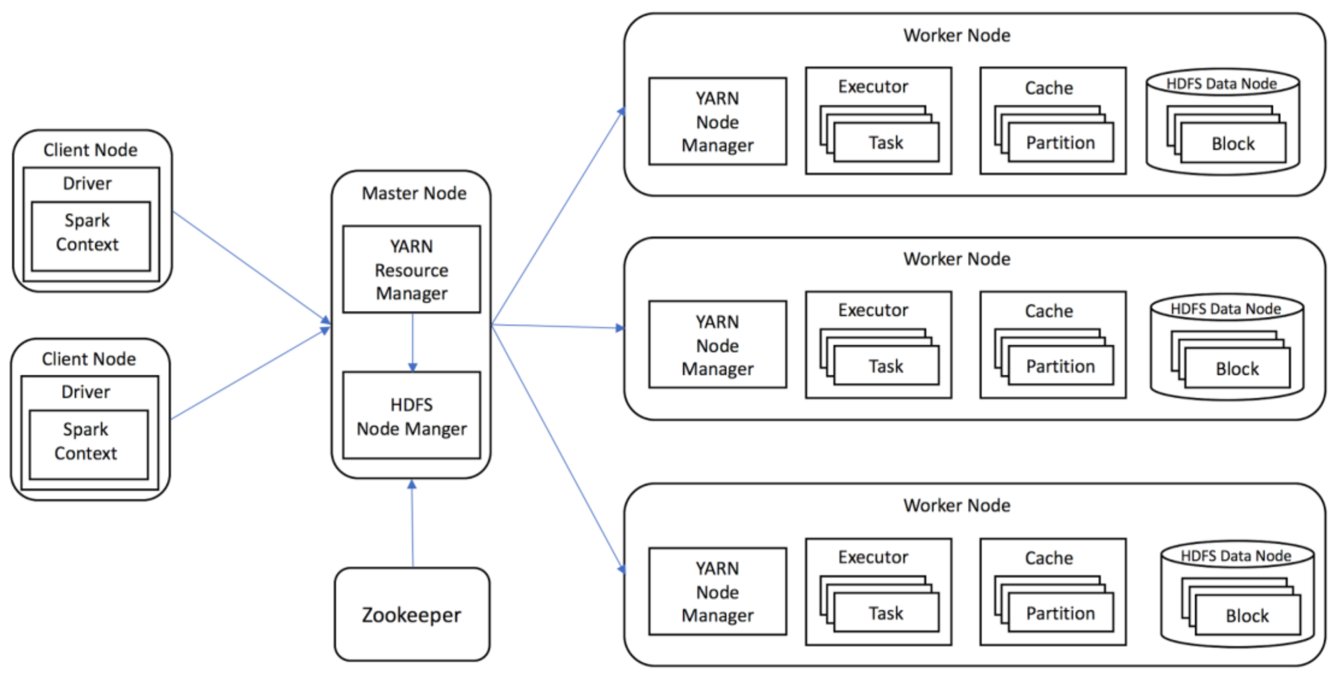
ClimateSpark stores the collection of arrays in HDF/NetCDF file, taking advantages of HDF/NetCDF (e.g., chunking, indexing, and hierarchical structure). ClimateSpark supports the regular chunking, and the chunks are stored in any order and any position within the file, enabling chunks to be read individually, while the cells in a chunk are stored in “row-major” order. ClimateSpark utilizes HDFS to get the scalable storage capability for fast increasing data volume. The HDF/NetCDF files are uploaded into HDFS without preprocessing. However, HDFS automatically splits a file into several blocks, usually 64 MB or 128 MB, and distributes them across the cluster. To better manage these chunks and improve data locality, ClimateSpark builds a spatiotemporal index to efficiently organize distributed chunks, and the index exactly identifies the chunk location information at the node, file, and byte. level. These characteristics greatly improves the partial I/O efficiency with high data locality and avoids unnecessary data reading.
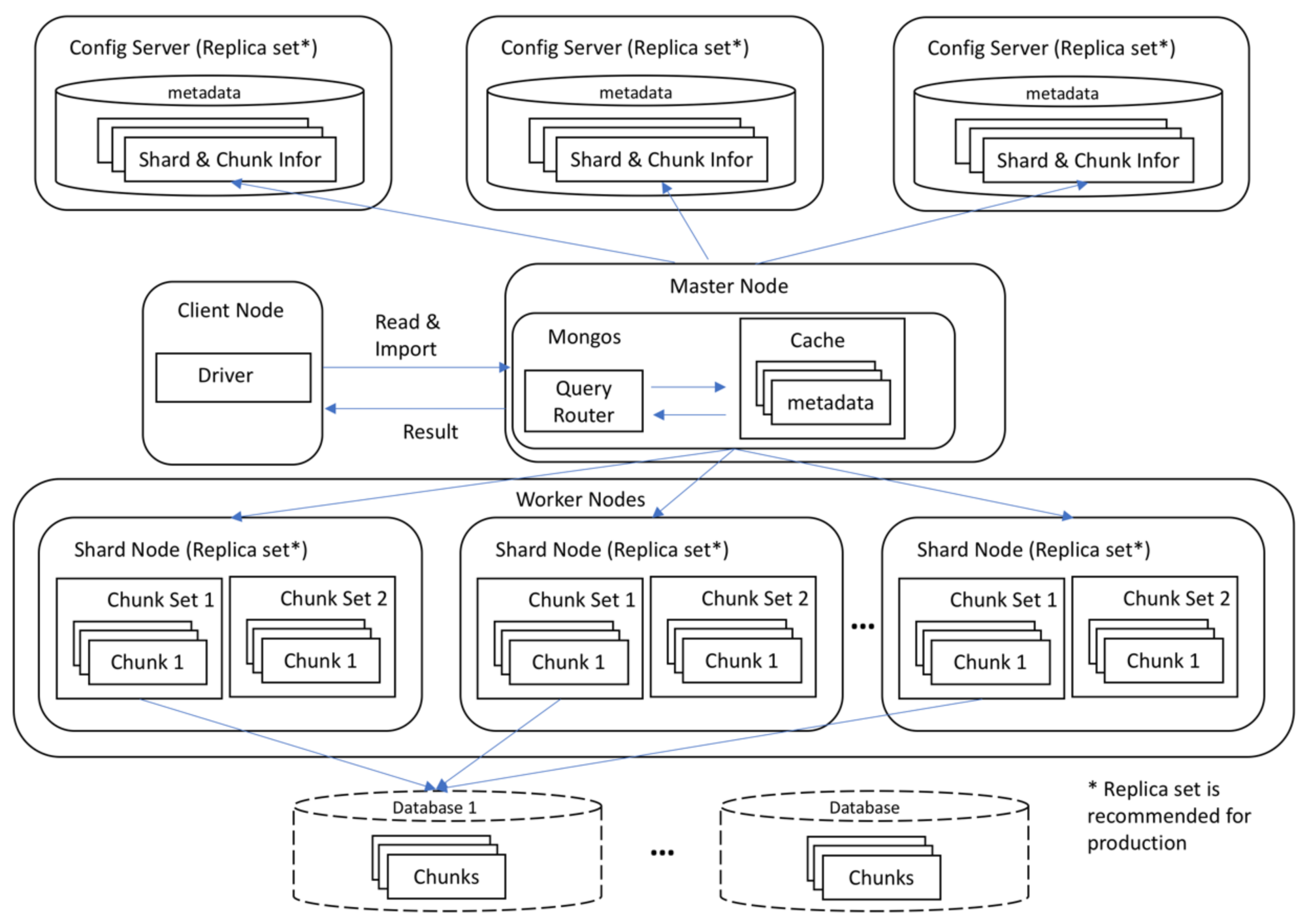
3.3.2. MongoDB

MongoDB does not support multidimensional data natively, and the array data need to be projected into key-value pairs and stored in a binary-encoded format called BSON behind the scenes. Chunking is achieved by splitting data into smaller pieces and spreading them equally among shard nodes in collection level. MongoDB supports chunking natively in sharding with a default size of 64 megabytes. However, smaller chunk sizes (e.g., 32 MB, 16 MB) is recommended for spreading the data more evenly across the shards. MongoDB defines indices at the collection level and supports indices on any field or sub-field of the documents [36]. It provides six types of indices: single field, compound, multi-key, geospatial, test and hashed index. The index is created automatically for the target field, irrespective of the kind of index performed. The purpose is to allow MongoDB to process and fulfill queries quickly by creating small and efficient representations of the documents in a collection [36]. Loading balance is conducted at chunk level to keep chunks equally distributed across the shard nodes.

3.3.3. Spark and Hive

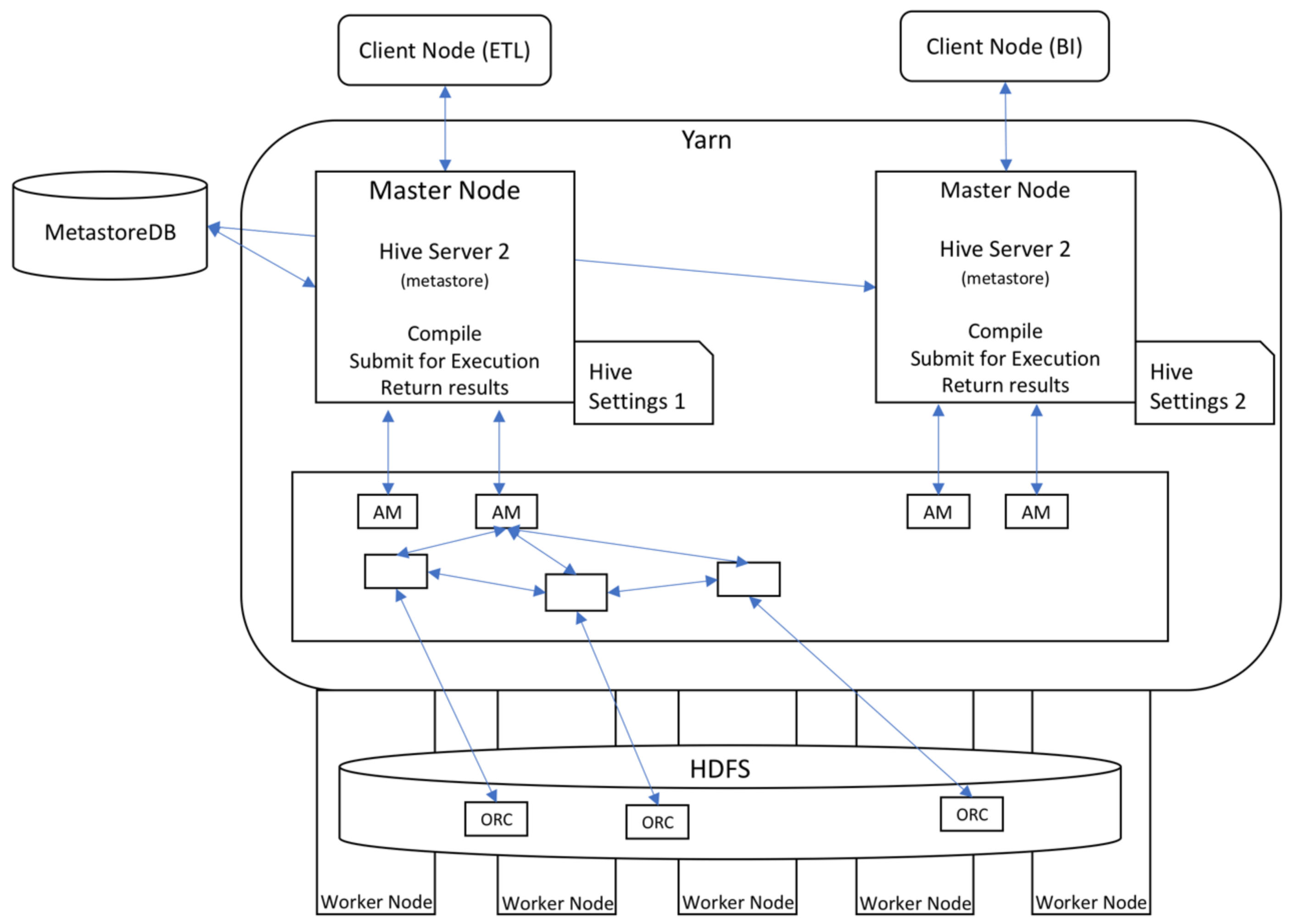
Spark and Hive leverage Parquet, a columnar storage format, to store the data in a relation table. Compared with the traditional row-oriented table (e.g., csv text files), Parquet is more disk saving and efficient in queries. In a Parquet table each column is stored and loaded separately, and this has two advantages: (1) the columns are efficiently compressed using the most suitable encoding schemes to save storage space; and (2) queries only need to read the specific columns rather than the entire rows. Meanwhile, each column is split into several column chunks with a column chunk containing one or more pages. The page is an indivisible unit in terms of compression and encoding and is composed of the header information and encoded values. Spark SQL and Hive SQL natively support Parquet files in HDFS and reads them with high data locality, an efficient and convenient way to query Parquet files in HDFS using Spark/Hive SQL.

3.4. Data Operations

Aiming to improve the usability and ease data operations, all containers develop their strategies for the users at different levels. However, these strategies (e.g., query language, API, extensibility, and support data format) are dissimilar (Table 5) due to their different design purpose and targeted user groups.
Spark and Hive need to convert the input array datasets into the support data formats (e.g., CSV and Parquet), but the projection coordination is kept in the relation table for geospatial queries. They also support the standard SQL and enable users to extend SQL functions by using user-defined-function APIs.
The ClimateSpark develops a HDFS-based middleware for HDF/NetCDF to natively support HDF and NetCDF datasets and keeps the projection information to support geospatial query. It provides the basic array operations (e.g., concatenation, average, max, conditional query) available at Spark-shell terminal in Scala API. The array can be visualized as PNG or GIF file. Users develop their own algorithms based on Scala and Java API. The Spark SQL is extended by using user-defined functions to support SQL operation on the geospatial data, but its operation is designed for the points rather than the array because Spark SQL does not support array data structure yet.
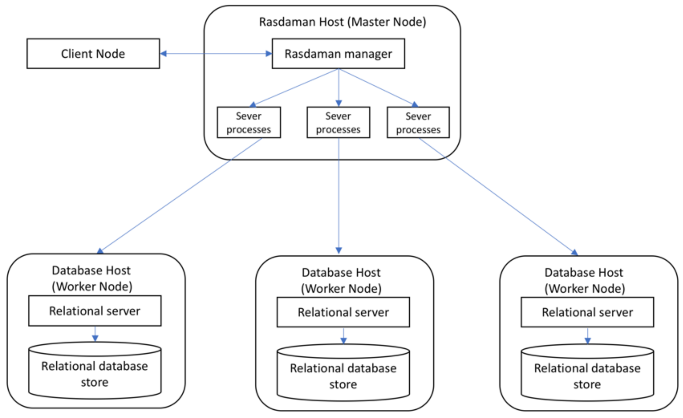
The Rasdaman provides the query language, rasql, to support retrieval, manipulation, and data definition (e.g., geometric operations, scaling, concatenation). It implements various data loading functions based on GDAL to natively support different raster data formats, including GeoTiff, NetCDF, and HDF. Users do not need to preprocess their original datasets, which are automatically loaded as multi-dimensional arrays. It also enables users to customize their functions via C++, Java, and Python API. However, it cannot automatically distribute the input data across the cluster, and users need to specify which data are loaded into which node. The project coordination information is lost after the data are imported.
The SciDB provides two query language interfaces, Array Functional Language (AFL) and prototype Array Query Language (AQL). Both work on the iquery client, a basic command line for connecting SciDB. Scripts for running AQL are similar to SQL for relational databases, while AFL is a functional language using operators to compose queries or statements. In AFL, operators are embedded according to user requirements, meaning each operator takes the output array of another operator as its input. The SciDB not only provides resourceful operators for satisfying users’ expectations, but it is also programmable from R and Python and support plugins as extension to better serve the needs (e.g., dev tools support installations of SciDB plugins from GitHub repositories). The CSV files, SciDB-formatted text, TSV files, and binary files are date formats currently supported by SciDB.
The query language in MongoDB is an object-oriented language, and similar to other NoSQL databases, it does not support join operation. Conversely, it supports dynamic queries on documents and is nearly as powerful as SQL. Since it is a schema-free database, the query language allows users to query data in a different manner which would have higher performance in some special cases. “Find” method in MongoDB, which is similar to “select” in SQL but limited to one table, is used to retrieve data from a collection. Different from traditional SQL, the query system in MongoDB is from top to bottom, operations take place inside a collection, and one collection contains millions of records. The MongoDB also supports aggregation operations, which groups values from multiple documents and performs as many operations as needed to return results. The aggregation framework is modeled on the concept of data processing pipelines [40]. Finally, map-reduce operation is supported, using custom JavaScript functions to perform map and reduce operations.

4. Experiment Design and Performance Evaluation

4.1. Experiment Setup and Design

4.1.1. Test Environment

To evaluate the performance of the data containers, each is deployed onto the same number of worker nodes. The cluster node is configured with 24 CPU cores (2.35 GHz) and 24 GB RAM on CentOS 7.2 and connected with 12 GB Ethernet (GPS). The architectures for the selected data containers are the following: (1) Spark (v1.5.2), Hive (v1.1.0), and ClimateSpark (v0.1) are deployed on the same Hadoop cluster consisting of one master node and 19 worker nodes; (2) Rasdaman (v9.4.0) contains 19 database nodes, with one serving as the Rasdaman host; (3) SciDB (v15.12) is deployed on a 19-node cluster, including a coordinator node; and (4) MongoDB (v3.2.4) cluster for the experiment is structured with 19 shard nodes, 3 Config nodes, and 1 mongos node (application node).

4.1.2. Experiment Design

To evaluate the performance of the selected data containers on large-scale, multi-dimensional array datasets, MOD08_D3, one of the Level-3 MODIS Atmosphere Daily Global Products from 1 March 2000 to 1 March 2016, is collected (about 1.1 TB) as the experiment data. The original MOD08_D3 dataset is stored in HDF4 format and contains about 974 variables with different dimensions (e.g., 3D, 4D, and 5D) to record the data for aerosol, water vapor, cloud, and atmosphere profile. The spatial resolution is 1 by 1 degree, and the temporal resolution is daily. Three 3D, 4D, and 5D variables are loaded into the containers, and their original compressed data size in the HDF files are 0.21 GB, 4.38 GB, and 1.09 GB, respectively. HDF format was chosen because of its representativeness in Earth observation and simulation. When the queries are conducted, they are performed by each container against the data in the container’s own format, in which the HDF data was preprocessed into when loading the data to the container.
The experiment considers the following five aspects as relevant for the data container benchmark: (1) the flexibility of the data model for presenting multidimensional array data; (2) the labor and time for loading data into containers; (3) the storage consumed for data pre-processing; (4) the expressive capability for implementing the specified queries; and (5) the run time and resources (e.g., CPU, memory, and network) consumed for retrieving the target datasets. To evaluate the data containers from the above aspects, data were first uploaded to each data container, and some data pre-processing work is required for the containers that do not natively support the HDF data format. Second, different spatiotemporal queries were designed to evaluate the performance of the selected data containers. Statistical computations such as average for the data specified in a certain spatial and temporal range is an essential step in processing geospatial raster data, and is considered as canonical operations in different research domains (e.g., GIS, remote sensing, and climate study) [41,42]. Therefore, the following three spatiotemporal queries are selected: (1) the point time series query for different time range; (2) the spatial-average query for the specified variable in different time range; and (3) the global-average query for the specified variable in different time range. The spatial coverages specified by the first point query and second spatial query refer to the data in Boulder City, CO and Colorado State (CO), USA, respectively. During these queries the consumed computing and storage resources are recorded using the Ganglia cluster.

4.2. Experiment Results and Analytics

4.2.1. Data Preprocessing and Uploading

ClimateSpark natively supports HDF and NetCDF data formats with no requirement for data preprocessing, whereas Spark SQL and Hive decompose the multi-dimensional variables into points with coordinate and value information and stores them in Parquet format. Although Rasdaman supports array-based data model, it reads the data from the original datasets and re-encodes them in a specific data format representation. The Rasdaman does not support the HDF data format used in the experiment data, requiring the data to be converted initially into NetCDF file. Subsequently it utilizes Rasdaman query language to import the data. When converting HDF files to NetCDF files, we cannot specify only the variables our experiment selects. That means we need to convert the whole datasets, so the time and data size in Table 5 for Rasdaman is for all the variables in the file rather than a single variable. Similarly, SciDB converts the HDF files to the data format supported (e.g., CSV, OPAQUE, SciDB-formatted text, and TSV files). Although the user community developed plugins to support direct HDF data loading, these do not work for the experimental environment in this study due to the library version conflict issue. MongoDB converts the HDF files into separated CSV files and import them to the shard nodes.
When uploading data, ClimateSpark, Spark, and Hive use HDFS commands to directly move the data into HDFS. The Rasdaman provides the query language to upload the data by specifying the tile size and the variable name, but the lack of automatically delivering the data across the cluster requires: (1) manual specification of the data node for each piece of the data; and (2) tracking of the data location externally. The SciDB requires users to specify the number of attributes for the initial array equal to the number of columns in the CSV file before data loading. After loading, the data are displayed as a one-dimensional array with a dimension representing the number of rows in the CSV file. Users can assign a re-dimension function, and map selected array attributes to dimensions and generate a new array with multi-dimension. The MongoDB provides an import tool for CSV and JSON format data which converts each row of the CSV file into one JSON document and imports the document into database. The field names are treated as the field keys in each document, and the rows from one CSV file are imported to the same collection of the target database. In this study, 17 CSV files are generated for each variable to hold 17 years of data. Each CSV file contains space dimensions and time series as the fields. After importing data into the cluster, the sharding function is enabled at the collection level to let the load balancer split and distribute raw data among the worker nodes.
The data preprocessing time and the intermediate data size for each data container (Table 6) shows that ClimateSpark does not need preprocessing. For Spark, Hive, SciDB, and MongoDB, the NetCDF java library extracts the selected 3D, 4D, and 5D variables from the raw dataset. The process is parallelized by splitting the raw dataset to several servers and preprocessing them separately. The time (Table 6) is the elapsed time the involved servers spend for each data container. MongoDB spent more time for 4D and 5D variables than SciDB since MongoDB adopts a more complex table structure but saves more disk space. Although Spark and Hive use the same data structure with SciDB, the intermediate datasets are stored in Parquet data format, compressing the data with high ratio, so data size is smaller than the CSV files used in SciDB. Rasdaman takes the most time and disk space to preprocess data because all variables in the HDF files need to be converted into NetCDF files (Table 7).
In terms of data uploading, ClimateSpark, Spark, and Hive upload the data into HDFS, which automatically makes three copies of the input data and equally distributes them across the cluster. ClimateSpark spends more time than Spark and Hive as it uploads the original HDF4 files into HDFS instead of just the three selected variables. The smaller data size in Hive and Spark versus ClimateSpark indicates that Parquet achieves a better compression ratio than HDF4. SciDB also spends a long time to upload data because it needs to re-dimension the input relation-based data into chunked arrays. The time for RasDaMan and SciDB to upload data are comparable, but the data size achieved in the Rasdaman cluster is 33.7%, 64.6%, and 125% larger than that for SciDB for the 3D, 4D, and 5D variables, respectively. The MongoDB spends the most time to load and rebalance data. The data rebalancing in MongoDB is time- and resource-consuming because the load balancer core inside MongoDB does not support multi-threads processing and requires data locks among three Config servers before the chunk move is initiated. Meanwhile, both the import function and chunking function fail occasionally when processing large numbers of chunks.

4.2.2. Runtime for the Spatiotemporal Query

● The spatiotemporal query for the 3D variables
In most queries, MongoDB and SciDB performed better than the Map-Reduce style based systems (e.g., ClimateSpark, Spark, and Hive, Figure 7). Spark and Hive are designed for batch processing rather than real-time processing because they need to dynamically allocate computing resource and launch executors for each new job. However, MongoDB and SciDB provide system optimization to support nearly real-time data queries. They work well when the queried datasets fit well the available memory of the cluster. However, their run-time gap decreases with an increase in the spatial and temporal range. For example, the run time for ClimateSpark to compute the global average for 16 years is even smaller than MongoDB and SciDB. This indicates that ClimateSpark more efficiently handles a large volume of data. For ClimateSpark and Spark, ClimateSpark performs better than Spark except for the one-year, four-year, and eight-year queries for the 3D variable and the one-year query for the 5D variable. Since Spark SQL does not support the index for Parquet file, it iterates all elements in a certain column to search the specified data and yet remains faster than ClimateSpark when querying small datasets. This indicates that Spark works better than ClimateSpark (Spark+HDF/NetCDF) with Parquet files for small data queries. When the queried data volume increases, ClimateSpark performs better than Spark, reflecting the high data locality achieved by the spatiotemporal index to avoid data shuffling. The default data aggregation strategy in Spark is not efficient for computing the average, which requires more data movement across the cluster to group the values by the specified dimensions. The Rasdaman performs better than Hive, Spark, and ClimateSpark when conducting the queries for Boulder and Colorado State, but its performance declines for the queries focused on global areas. Two reasons are offered to explain this pattern. The first is that the global queries combine the separated chunks which increases the query time on each Rasdaman worker node. The second is that Rasdaman does not support parallel query resulting in the queries running in sequence rather than in parallel. Hive spends more time than other platforms, but Hive SQL greatly reduces the difficulties for users to run MapReduce jobs.
● The spatiotemporal query for the 4D variable
The number of points in the 4D variable is 30 times larger than that of the 3D variable. At the beginning SciDB and MongoDB have performed better than Spark, ClimateSpark, Hive, and Rasdaman, but their query times increase faster than the others when the spatiotemporal query bounding box is enlarged. In the third group of experiments (Figure 8c), Spark and ClimateSpark spend less time than the others for computing the global mean value. The following five reasons are offered to explain this pattern. First, Spark and ClimateSpark handle more effectively the situation when the queried data do not fit in memory by serializing the data into disk. Second, ClimateSpark directly aggregates the chunks contained by the bounding box instead of iterating each point. Third, MongoDB memory maps all the data and is fast for caching small dataset but slows dramatically when the queried data size exceeds available memory. Fourth, SciDB is the first to navigate to the chunk (s) location according to the query using the chunk hash indexes. When there is growth of the size of a bounding box, more chunks are needed, causing a smooth and steady time increase. Fifth, each node in Rasdaman needs more time to query large volume of data while the queries are conducted in sequence on each node rather than in parallel.
● The spatiotemporal query for the 5D variable
The 5D variable has 72 times the number of points of the 3D variable (Figure 9). The SciDB has a similar high query performance for the point queries (<3 s) and area queries (1.2–7.6 s), but the run time for computing the global mean value increased from 44.3 s to 649.2 s. The performance of MongoDB declines more than SciDB [43]. For the point query, the run time increases from 0.5 s to 3.9 h, three times more than that of Hive (1.1 h). This performance repeatedly happens in the area and global queries because the query target of 5D dataset exceeds the available physical memory of current system, slowing dramatically as it is disk bound. For Rasdaman, there is a similar run-time trend in the point- and area-queries. In contrast, the containers in the Hadoop ecosystem (ClimateSpark, Spark, and Hive) are more stable in their performance. The runtime for ClimateSpark increases from 7.9 to 83.9 s for the point query, 8 to 86.6 s for the area query, and 10 to 94.3 s for the global query at an increasing rate <2. The performance of Spark is better than that of ClimateSpark when the query time is >4 years, indicating that Spark supports the Parquet format (e.g., decompression, query, and shuffling) well for large volume of data processing. Since pure Spark does not support indices, ClimateSpark performs better when querying a small piece of data from large datasets. Hive’s performance is also stable and the run time faster than MongoDB when the query time range is >12 years.

4.2.3. Resource Consumption for Different Queries

To measure the efficiency of resources usage in different data containers, the resources consumed for the experiments on the 3D variable (e.g., CPU, memory, and network) were recorded (Figure 10). The average resource consumption per node for the data containers are recorded where Q1, Q2, and Q3 represent the point query, area query, and global query, respectively. All data containers consume more memory with the enlarged spatiotemporal bounding box, but they increase at different rates. Although MongoDB and SciDB consume less memory on these three types of queries, the memory size increases exponentially for the global query (Q3). This indicates that MongoDB and SciDB are not as effective as Spark and Hive at memory management when querying large datasets. Notably, Spark and ClimateSpark for Q3 consume less memory than Q2, a consequence of the chunking structure, which aggregate the chunks instead of visiting each point. Comparing the CPU consumption, Rasdaman, Hive, Spark, and ClimateSpark use more CPUs than MongoDB and SciDB because they need to decompress the data on the fly. The combination of bytes-in and bytes-out measures how data are transferred across the cluster. This pattern is attributed to the ease of moving the code to the data which is more efficient than moving data to the code, a key point for the speed of querying large volume of data. The MongoDB, Rasdaman, and SciDB have less data being transferred over the network. With chunk location information, ClimateSpark consumes less bandwidth than Spark does. Based on the above, several conclusions are offered. First, MongoDB and SciDB are more efficient on CPU and network. Second, Hive, Spark, and ClimateSpark have better strategies to utilize the memory for increasing query bounding box. Third, the spatiotemporal index in ClimateSpark improves the data locality of Spark to reduce the data transferring via the network.

5. Conclusion and Future Work

This research evaluates the capability of the popular data containers (i.e., Spark, ClimateSpark, Hive, Rasdaman, SciDB, and MongoDB) for handling geospatial raster data. Run time and consumed resources are used as metrics to measure their performance for different types of spatiotemporal queries [39,44]. These data containers are compared and evaluated from two perspectives: (a) their system design and architecture (i.e., distributed architecture, logical data model, physical data model, and data operations) (Table 2, Table 3, Table 4 and Table 5); and (b) their practical use experience and performance (i.e., data preprocess, data uploading, query, resource consumption, and extendibility) (Table 6, Table 7 and Table 8). The extendibility is measured based on the documents provided on their project websites, the code examples in their user community, and the number of related publications that extend their system.
From the experimental result, six general conclusions are offered.
  • Data preprocessing is time- and resource-consuming, especially for large volumes of data. Unfortunately, as of the publication of the paper, all the data containers, except ClimateSpark, convert HDF files to other data formats for data uploading. SciDB and MongoDB are very time-consuming to reorganize and rebalance the uploaded data. ClimateSpark has a spatiotemporal index to enable Spark to natively support HDF files to avoid the data preprocessing process.
  • SciDB and MongoDB have better query performance, with nearly real-time to responses to users’ small/medium bounding boxes, but their performance is limited when handling large data volumes due to their heavy consumption of memory.
  • Spark and ClimateSpark handle large volumes of data efficiently with stable resource consumption.
  • SciDB and Rasdaman provide a mature array-based data operation and analytical functions, whereas Hive, MongoDB, Spark, and ClimateSpark lack these functions. Specifically, for MongoDB, complicated scripts are required to implement simple spatiotemporal queries.
  • Hive, Spark, ClimateSpark, SciDB, and MongoDB automatically run queries in parallel, but Rasdaman requires manual intervention to write the queries for different nodes and does not support parallel query.
  • SciDB, Spark, Hive, and ClimateSpark support the user defined functions to extend the system capability, which helps users develop their customized functions.
The results are evaluated based on the average resulting value by repeating the same experiments 10 times. For all the experiments, hardware and baseline software, such as operational systems, are the same. Therefore, the result is credible for general conclusion. However, the results might be different when different hardware or baseline software are used. For example, results would be different when the network speed or the disk I/O speed is different because of the change of potential bottlenecks of a data container. Further optimization of different data containers might help improve their performance.
Nevertheless, based on the above conclusions, we find that none of the six selected data containers could meet all the requirements of different geospatial raster data applications. That means a hybrid solution would be helpful to obtain best performance for big geospatial raster data management. The following four research directions are proposed to develop a hybrid framework: (1) evaluate more state-of-the-art data containers (e.g., Cassandra and Open Data Cube) to provide readers with more reference information; (2) enhance the data containers to enable loading automatically geospatial data to avoid complex data preprocessing; (3) design a strategy to efficiently leverage the different characteristics of these containers to better manage and query geospatial data (for example, MongoDB and SciDB could be used to process real time query of small data volume, while Spark and ClimateSpark could be used to process large volumes of data in batch mode); and (4) develop a web portal to enable users to submit queries remotely and visualize the results online.

Acknowledgments

This project is funded by NASA AIST (NNX15AM85G) and NSF (IIP-1338925 and ICER-1540998). We thank the anonymous reviewers for their insightful comments and reviews. ClimateSpark was developed by Fei Hu, Michael Bowen, Daniel Duffy, Chaowei Yang and others. George Taylor helped proofread the manuscript.

Author Contributions

Chaowei Yang, Michael Little, and Christopher Lynnes came up with the original research idea; Chaowei Yang advised Fei Hu, Mengchao Xu, and Jingchao Yang on the experiment design and paper structure; Fei Hu, Mengchao Xu, and Jingchao Yang designed the experiments, deployed the experiment environment, developed the scripts for experiments, conducted the experiments, and analyzed the experiment results; Yanshou Liang developed the Ganglia monitoring system and developed the scripts for automatically monitoring the specified running tasks; Kejin Cui cleaned and visualized the resource monitoring data; Fei Hu, Mengchao Xu, and Jingchao Yang wrote the paper; and Chaowei Yang revised the paper.

Conflicts of Interest

The authors declare no conflict of interest.

References

  1. Demchenko, Y.; Grosso, P.; De Laat, C.; Membrey, P. Addressing big data issues in scientific data infrastructure. In Proceedings of the 2013 International Conference on Collaboration Technologies and Systems (CTS), San Diego, CA, USA, 20–24 May 2013; pp. 48–55. [Google Scholar]
  2. Lynch, C. Big data: How do your data grow? Nature 2008, 455, 28–29. [Google Scholar] [CrossRef] [PubMed]
  3. Camara, G.; Assis, L.F.; Ribeiro, G.; Ferreira, K.R.; Llapa, E.; Vinhas, L. Big earth observation data analytics: Matching requirements to system architectures. In Proceedings of the 5th ACM SIGSPATIAL International Workshop on Analytics for Big Geospatial Data, Burlingame, CA, USA, 31 October 2016; ACM: New York, NY, USA, 2016; pp. 1–6. [Google Scholar]
  4. Skytland, N. What Is NASA Doing with Big Data Today? 2012. Available online: https://open.nasa.gov/blog/what-is-nasa-doing-with-big-data-today/ (accessed on 6 April 2018).
  5. Das, K. Evaluation of Big Data Containers for Popular Storage, Retrieval, and Computation Primitives in Earth Science Analysis. In Proceedings of the 2015 AGU Fall Meeting Abstracts, San Francisco, CA, USA, 14–18 September 2015. [Google Scholar]
  6. Yang, C.; Huang, Q.; Li, Z.; Liu, K.; Hu, F. Big Data and cloud computing: Innovation opportunities and challenges. Int. J. Digit. Earth 2017, 10, 13–53. [Google Scholar] [CrossRef]
  7. National Research Council. IT Roadmap to a Geospatial Future; National Academies Press: Washington, DC, USA, 2003. [Google Scholar]
  8. Baumann, P.; Stamerjohanns, H. Towards a systematic benchmark for array database systems. In Specifying Big Data Benchmarks; Springer: Berlin/Heidelberg, Germany, 2014; pp. 94–102. [Google Scholar]
  9. Brown, P.G. Overview of SciDB: Large scale array storage, processing and analysis. In Proceedings of the 2010 ACM SIGMOD International Conference on Management of Data, Indianapolis, IN, USA, 6–11 June 2010; ACM: New York, NY, USA, 2010; pp. 963–968. [Google Scholar]
  10. Chodorow, K. MongoDB: The Definitive Guide: Powerful and Scalable Data Storage; O’Reilly Media, Inc.: Beijing, China, 2013. [Google Scholar]
  11. Thusoo, A.; Sarma, J.S.; Jain, N.; Shao, Z.; Chakka, P.; Anthony, S.; Liu, H.; Wyckoff, P.; Murthy, R. Hive: A warehousing solution over a map-reduce framework. Proc. VLDB Endow. 2009, 2, 1626–1629. [Google Scholar] [CrossRef]
  12. Zaharia, M.; Xin, R.S.; Wendell, P.; Das, T.; Armbrust, M.; Dave, A.; Meng, X.; Rosen, J.; Venkataraman, S.; Franklin, M.J.; et al. Apache Spark: A unified engine for big data processing. Commun. ACM 2016, 59, 56–65. [Google Scholar] [CrossRef]
  13. Rusu, F.; Cheng, Y. A survey on array storage, query languages, and systems. arXiv, 2013; arXiv:1302.0103. [Google Scholar]
  14. Davies, D.K.; Ilavajhala, S.; Wong, M.M.; Justice, C.O. Fire information for resource management system: Archiving and distributing MODIS active fire data. IEEE Trans. Geosci. Remote Sens. 2009, 47, 72–79. [Google Scholar] [CrossRef]
  15. Zhong, Y.; Sun, S.; Liao, H.; Zhao, Y.; Fang, J. A novel method to manage very large raster data on distributed key-value storage system. In Proceedings of the 2011 19th International Conference on Geoinformatics, Shanghai, China, 24–26 June 2011; pp. 1–6. [Google Scholar]
  16. MySQL Enterprise Scalbility. Available online: https://www.mysql.com/products/enterprise/scalability.html (accessed on 6 April 2018).
  17. Obe, R.O.; Hsu, L.S. PostGIS in Action; Manning Publications Co.: Shelter Island, NY, USA, 2015. [Google Scholar]
  18. Zhong, Y.; Han, J.; Zhang, T.; Fang, J. A distributed geospatial data storage and processing framework for large-scale WebGIS. In Proceedings of the 2012 20th International Conference on Geoinformatics (GEOINFORMATICS), Hong Kong, China, 15–17 June 2012; pp. 1–7. [Google Scholar]
  19. Huang, Q.; Yang, C.; Liu, K.; Xia, J.; Xu, C.; Li, J.; Gui, Z.; Sun, M.; Li, Z. Evaluating open-source cloud computing solutions for geosciences. Comput. Geosci. 2013, 59, 41–52. [Google Scholar] [CrossRef]
  20. Yang, C.; Yu, M.; Hu, F.; Jiang, Y.; Li, Y. Utilizing Cloud Computing to address big geospatial data challenges. Comput. Environ. Urban Syst. 2017, 61, 120–128. [Google Scholar] [CrossRef]
  21. Hu, H.; Wen, Y.; Chua, T.S.; Li, X. Toward scalable systems for big data analytics: A technology tutorial. IEEE Access 2014, 2, 652–687. [Google Scholar]
  22. Zhang, Y.; Kersten, M.; Manegold, S. SciQL: Array data processing inside an RDBMS. In Proceedings of the 2013 ACM SIGMOD International Conference on Management of Data, New York, NY, USA, 22–27 June 2013; ACM: New York, NY, USA, 2013; pp. 1049–1052. [Google Scholar]
  23. Geng, Y.; Huang, X.; Zhu, M.; Ruan, H.; Yang, G. SciHive: Array-based query processing with HiveQL. In Proceedings of the 2013 12th IEEE International Conference on Trust, Security and Privacy in Computing and Communications (TrustCom), Melbourne, VIC, Australia, 16–18 July 2013; pp. 887–894. [Google Scholar]
  24. Aji, A.; Wang, F.; Vo, H.; Lee, R.; Liu, Q.; Zhang, X.; Saltz, J. Hadoop GIS: A high performance spatial data warehousing system over mapreduce. Proc. VLDB Endow. 2013, 6, 1009–1020. [Google Scholar] [CrossRef]
  25. Palamuttam, R.; Mogrovejo, R.M.; Mattmann, C.; Wilson, B.; Whitehall, K.; Verma, R.; McGibbney, L.; Ramirez, P. SciSpark: Applying in-memory distributed computing to weather event detection and tracking. In Proceedings of the 2015 IEEE International Conference on Big Data (Big Data), Santa Clara, CA, USA, 29 October–1 November 2015; pp. 2020–2026. [Google Scholar]
  26. Baumann, P.; Dehmel, A.; Furtado, P.; Ritsch, R.; Widmann, N. The multidimensional database system RasDaMan. In Proceedings of the 1998 ACM SIGMOD International Conference on Management of Data, Seattle, WA, USA, 1–4 June 1998; ACM: New York, NY, USA, 1998; Volume 27, pp. 575–577. [Google Scholar]
  27. Chock, M.; Cardenas, A.F.; Klinger, A. Database structure and manipulation capabilities of a picture database management system (PICDMS). IEEE Trans. Pattern Anal. Mach. Intell. 1984, 6, 484–492. [Google Scholar] [CrossRef] [PubMed]
  28. Kersten, M.; Zhang, Y.; Ivanova, M.; Nes, N. SciQL, a query language for science applications. In Proceedings of the EDBT/ICDT 2011 Workshop on Array Databases, Uppsala, Sweden, 25 March 2011; ACM: New York, NY, USA, 2011; pp. 1–12. [Google Scholar]
  29. Cudré-Mauroux, P.; Kimura, H.; Lim, K.T.; Rogers, J.; Simakov, R.; Soroush, E.; Velikhov, P.; Wang, D.L.; Balazinska, M.; Becla, J.; et al. A demonstration of SciDB: A science-oriented DBMS. Proc. VLDB Endow. 2009, 2, 1534–1537. [Google Scholar] [CrossRef]
  30. Planthaber, G.; Stonebraker, M.; Frew, J. EarthDB: Scalable analysis of MODIS data using SciDB. In Proceedings of the 1st ACM SIGSPATIAL International Workshop on Analytics for Big Geospatial Data, Redondo Beach, CA, USA, 6 November 2012. [Google Scholar]
  31. Amirian, P.; Basiri, A.; Winstanley, A. Evaluation of data management systems for geospatial big data. In Proceedings of the International Conference on Computational Science and Its Applications, Guimarães, Portugal, 30 June–3 July 2014; Springer International Publishing: Cham, Switzerland, 2014; pp. 678–690. [Google Scholar]
  32. Aniceto, R.; Xavier, R.; Holanda, M.; Walter, M.E.; Lifschitz, S. Genomic data persistency on a NoSQL database system. In Proceedings of the 2014 IEEE International Conference on Bioinformatics and Biomedicine (BIBM), Belfast, UK, 2–5 November 2014; pp. 8–14. [Google Scholar]
  33. Ameri, P.; Grabowski, U.; Meyer, J.; Streit, A. On the application and performance of MongoDB for climate satellite data. In Proceedings of the 2014 IEEE 13th International Conference on Trust, Security and Privacy in Computing and Communications (TrustCom), Beijing, China, 24–26 September 2014; pp. 652–659. [Google Scholar]
  34. Han, D.; Stroulia, E. Hgrid: A data model for large geospatial data sets in hbase. In Proceedings of the 2013 IEEE Sixth International Conference on Cloud Computing (CLOUD), Santa Clara, CA, USA, 28 June–3 July 2013; pp. 910–917. [Google Scholar]
  35. Merticariu, G.; Misev, D.; Baumann, P. Towards a General Array Database Benchmark: Measuring Storage Access. In Big Data Benchmarking; Springer: Cham, Switzerland, 2015; pp. 40–67. [Google Scholar]
  36. Indexes. 2017. Available online: https://docs.mongodb.com/manual/indexes/ (accessed on 6 April 2018).
  37. Aggregation. 2017. Available online: https://docs.mongodb.com/manual/aggregation/ (accessed on 6 April 2018).
  38. Chevalier, M.; El Malki, M.; Kopliku, A.; Teste, O.; Tournier, R. Implementation of multidimensional databases with document-oriented NoSQL. In Proceedings of the International Conference on Big Data Analytics and Knowledge Discovery, Valencia, Spain, 1–4 September 2015; Springer International Publishing: Cham, Switzerland, 2015; pp. 379–390. [Google Scholar]
  39. Gudivada, V.N.; Rao, D.; Raghavan, V.V. NoSQL systems for big data management. In Proceedings of the 2014 IEEE World Congress on Services (SERVICES), Anchorage, AK, USA, 27 June–2 July 2014; pp. 190–197. [Google Scholar]
  40. Compare to Relational Database. Available online: http://www.paradigm4.com/try_scidb/compare-to-relational-databases/ (accessed on 6 April 2018).
  41. Li, Z.; Hu, F.; Schnase, J.L.; Duffy, D.Q.; Lee, T.; Bowen, M.K.; Yang, C. A spatiotemporal indexing approach for efficient processing of big array-based climate data with MapReduce. Int. J. Geogr. Inf. Sci. 2017, 31, 17–35. [Google Scholar] [CrossRef]
  42. Schnase, J.L.; Duffy, D.Q.; Tamkin, G.S.; Nadeau, D.; Thompson, J.H.; Grieg, C.M.; McInerney, M.A.; Webster, W.P. MERRA analytic services: Meeting the big data challenges of climate science through cloud-enabled climate analytics-as-a-service. Comput. Environ. Urban Syst. 2017, 61, 198–211. [Google Scholar] [CrossRef]
  43. Stonebraker, M.; Brown, P.; Zhang, D.; Becla, J. SciDB: A database management system for applications with complex analytics. Comput. Sci. Eng. 2013, 15, 54–62. [Google Scholar] [CrossRef]
  44. Yang, C.; Wu, H.; Huang, Q.; Li, Z.; Li, J. Using spatial principles to optimize distributed computing for enabling the physical science discoveries. Proc. Natl. Acad. Sci. 2011, 14, 5498–5503. [Google Scholar] [CrossRef] [PubMed]
Figure 1. The general architecture for distributed data storage and processing.
Ijgi 07 00144 g001
Figure 2. The architecture of Spark.
Ijgi 07 00144 g002
Figure 3. The architecture of Hive.
Ijgi 07 00144 g003
Figure 4. The architecture of Rasdaman.
Ijgi 07 00144 g004
Figure 5. The architecture of SciDB.
Ijgi 07 00144 g005
Figure 6. The architecture of MongoDB.
Ijgi 07 00144 g006
Figure 7. The spatiotemporal query for the 3D variable at : (a) the point (Boulder) time series query by varying the time range; (b) the area average for the Colorado State by varying the time range; and (c) the global average by varying the time range.
Ijgi 07 00144 g007
Figure 8. The spatiotemporal query for the 4D variable at: (a) the point (Boulder) time series query by varying the time range; (b) the area average for the Colorado State by varying the time range; and (c) the global average by varying the time range.
Ijgi 07 00144 g008aIjgi 07 00144 g008b
Figure 9. The spatiotemporal query for the 5D variable at: (a) the point (Boulder) time series query by varying the time range; (b) the area average for the Colorado State by varying the time rang; and (c) the global average by varying the time range.
Ijgi 07 00144 g009
Figure 10. Resource monitoring result for the spatiotemporal query experiment on the 3D variable for 16 years: (a) average memory consumption; (b) average CPU consumption; (c) average byte-in volume; and (d) average bytes-out volume.
Ijgi 07 00144 g010
Table 1. The specific terminologies the data containers use for client node, master node, and worker/data nodes.
Client NodeMaster NodeWorker/Data Node
Spark/ClimateSparkSpark driver, Spark contextYARN resource manager, HDFS managerYARN node manager, Executor, HDFS data node
HiveHive clientHive sever, Tez Application Master, YARN resource manager, HDFS managerYARN node manager, Executor, HDFS data node
RasdamanRasdaman clientRasdaman host/managerDatabase host
SciDBSciDB clientCoordinator nodeWorker node
MongoDBMongoDB clientMongos, Query routerShard node
Table 2. The logical data model comparison between Rasdaman, SciDB, and ClimateSpark.
Dimension SizeProjectionData Type
Rasdamanflexiblenot supportbase/composite
SciDBflexiblesupportbase/composite
ClimateSparkflexiblesupportbase
Table 3. The graphic illustration of the logical data models.
Logical Data Model
Rasdaman/SciDB/ClimateSpark Ijgi 07 00144 i001
Spark/Hive Ijgi 07 00144 i002
MongoDB Ijgi 07 00144 i003
Table 4. The physical data model comparison between Spark, ClimateSpark, Hive, Rasdaman, SciDB, and MongoDB.
ChunkingIndexesData FormatDistributed Storage
Spark/Hivecolumnar-based chunkingno indexParquet + HDFSautomatically
ClimateSparkregular chunkingB-treeHDF/NetCDF + HDFSautomatically
Rasdamanregular, aligned, tiling areas of interestr+, directory index, regular computed indexPostgreSQLmanually
SciDBoverlapped chunkinghash-tableSpecific binary formatautomatically
MongoDBregular chunkingsingle field indexes, compound indexes, multikey indexes, geospatial indexes, test indexes and hashed indexBSONautomatically
Table 5. The data operation comparison for Spark, ClimateSpark, Hive, Rasdaman, SciDB, and MongoDB.
Query LanguageAPIExtensibleSupport Data Format
SparkSpark SQLJava/ScalaEasyParquet, CSV
ClimateSparkSQL, ScalaJava, ScalaEasyNetCDF, HDF, Parquet, CSV
HiveHiveQLJavaEasyParquet, CSV
RasdamanRasqlC++, Java, PythonDifficultNetCDF, HDF, GeoTiff, CSV
SciDBAFL, AQLiquery client, C++, Java, Python, REasyCSV, SciDB-formatted Text, TSV, Binary File
MongoDBScriptJava, Python, C++DifficultCSV, JSON
Table 6. Data Preprocessing Time and Intermediate Data Size.
Time (hour)Data Size (GB)
3D4D5D3D4D5D
ClimateSparkn/pn/pn/pn/pn/pn/p
Spark1.586.979.500.154.21
Hive1.586.979.500.154.21
Rasdaman 73.10 1740.8
SciDB1.637.5811.2513.9218.2627.1
MongoDB0.1811.3324.082.654208
Table 7. Data Uploading Time and Data Size in Container.
Time (hour)Data Size (GB)
3D4D5D3D4D5D
ClimateSpark 9.7 0.6313.143.27
Spark0.20.360.500.4412.53.1
Hive0.20.360.500.4412.53.1
Rasdaman8.628.450.3131.7145.2134.4
SciDB3224923.788.259.7
MongoDB6.2101.33525.0113.6164.2
Table 8. Comparison of the data containers’ practical user experience and performance.
Data PreprocessingParallel QueryResource ConsumptionData OperationExtendibility
CPUMemoryNetwork
SciDBYesGoodGoodGoodGoodGoodGood
RasdamanYesPoorFairFairFairGoodFair
MongoDBYesGoodGoodGoodGoodPoorFair
HiveYesFairPoorPoorPoorFairGood
ClimateSparkNoGoodPoorGoodFairFairFair
SparkYesGoodPoorGoodPoorFairGood

