Environmental Influences on Leisure-Time Physical Inactivity in the U.S.: An Exploration of Spatial Non-Stationarity


1
Department of Geography and Geographic Information Science, University of Illinois at Urbana-Champaign, Natural History Building, MC-150, 1301 W Green Street, Urbana, IL 61801, USA
2
Illinois Informatics Institute, University of Illinois at Urbana-Champaign, National Center for Supercomputing Applications, MC-257, 1205 W Clark St., Urbana, IL 61801, USA
*
Author to whom correspondence should be addressed.
ISPRS Int. J. Geo-Inf. 2018, 7(4), 143; https://doi.org/10.3390/ijgi7040143
Submission received: 13 February 2018
/
Revised: 26 March 2018
/
Accepted: 2 April 2018
/
Published: 5 April 2018
(This article belongs to the Special Issue Geoprocessing in Public and Environmental Health)
Abstract
:Considerable research has been conducted to advance our understanding of how environmental factors influence people’s health behaviors (e.g., leisure-time physical inactivity) at the neighborhood level. However, different environmental factors may operate differently at different geographic locations. This study explores the inconsistent findings regarding the associations between environmental exposures and physical inactivity. To address spatial autocorrelation and explore the impact of spatial non-stationarity on research results which may lead to biased estimators, this study uses spatial regression models to examine the associations between leisure-time physical inactivity and different social and physical environmental factors for all counties in the conterminous U.S. By comparing the results with the conventional ordinary least squares regression and spatial lag model, the geographically weighted regression model adequately addresses the problem of spatial autocorrelation (Moran’s I of the residual = 0.0293) and highlights the spatial non-stationarity of the associations. The existence of spatial non-stationarity that leads to biased estimators, which were often ignored in past research, may be another reason for the inconsistent findings in previous studies besides the modifiable areal unit problem and the uncertain geographic context problem. Also, the observed associations between environmental variables and leisure-time physical inactivity are helpful for developing location-based policies and interventions to encourage people to undertake more physical activity.
1. Introduction
For decades, researchers in public health and preventive medicine have examined the effects of environmental exposures on various health problems. There is growing evidence that indicates the association between environmental exposures and health outcomes [1,2,3,4]. Concerns about how the environment influences human health have attracted increasing attention with the increasing use of advanced spatial analytical methods and geographic information science (GIS) [5]. In environmental health research, many researchers are interested in physical inactivity [6,7,8] and its influence on chronic diseases, such as type-II diabetes, obesity, and cardiovascular diseases [9,10,11,12,13]. Physical inactivity includes leisure-time physical inactivity (LTPI) and non-leisure-time physical inactivity (NLTPI) [14]. Previous studies have found that both LTPI and NLTPI are affected by environmental contexts [15,16,17,18,19,20,21,22].
Considerable research has been conducted to advance our understanding of how physical environmental factors [20,23,24,25,26,27,28,29,30,31,32,33,34,35,36,37,38,39,40] and social environmental factors [19,28,41,42,43,44,45,46] influence people’s physical inactivity. In many of these studies, however, environmental determinants are found to have inconsistent associations with physical inactivity [22,28,31,45,46,47,48]. For example, some previous studies have not found any significant association between physical inactivity and weather, which however is one of the perceived factors that influence physical inactivity [22,47,48]. The access to, density of, or proximity to parks have been found to be related to physical inactivity in some studies while unrelated in other studies [20,25,49,50,51,52,53]. Similar inconsistent results were also found in the exposure to recreation facilities [49,50,51,52,54,55], street connectivity [20,25,30,50,56,57,58,59], and crime-related safety [49,51,55].
Scholars have attributed such inconsistency to the modifiable areal unit problem (MAUP) [60,61,62] and the uncertain geographic context problem (UGCoP) [63,64,65,66]. For example, the correlations found at various spatial scales (e.g., neighborhood, city, county, and state levels) may be different [60]. Furthermore, the different delineations of contextual areas (e.g., census tracts, home buffers, road network buffers) used to derive contextual or exposure measures may also affect the results [67,68]. Nevertheless, even at the same spatial scale and using the same exposure assessment method, environmental factors may operate differently at different geographic locations (a phenomenon known as spatial non-stationarity, which has been largely ignored in previous studies). For instance, street connectivity may be positively correlated with physical inactivity in one city while negatively associated with physical inactivity in another town. To the best of our knowledge, the spatial non-stationarity of environmental effects on physical inactivity and its influence on the consistency of research findings have not been adequately explored in previous studies and thus are worthy of investigation.
To fill the research gap, this paper seeks to explore the inconsistent findings regarding the associations between LTPI and different contextual variables (physical, demographic, and socioeconomic environmental factors) from the perspective of spatial non-stationarity. As an exploratory and ecological study, we examine the spatial variation of environmental effects on LTPI (percentage of population reporting insufficient leisure-time physical activity) at the spatial scale of U.S. counties. Previous studies have examined environmental effects on LTPI at the county level. However, none of these studies has considered the spatial autocorrelation in physical inactivity among neighboring counties as well as the existence of spatial non-stationarity [41,42,69,70]. Although both LTPI and NLTPI have been found to be associated with environmental factors, this study only focuses on environmental effects on LTPI to explore spatial non-stationarity and illustrate its influence on the results. By adopting a cross-sectional approach, the data in this research were collected in 2011. Further, the LTPI from nearby geographic units may have similar values, and spatial dependencies may exist (a phenomenon is known as spatial autocorrelation). To address the problem of spatial autocorrelation and investigate the existence of spatial non-stationarity, this study employs spatial regression models such as the spatial lag model (SLM) and geographically weighted regression (GWR). The result of this study shows that the relationships between contextual variables and LTPI are varied across geographic space at the county level, which indicates the existence of spatial non-stationarity. This study contributes to a better understanding of the environmental influences on LTPI and how these associations vary with geographic locations.
2. Materials and Methods
This research examines the relationships between LTPI and various environmental influences in the 3109 counties of the 48 contiguous states in the U.S. It uses county as the geographic unit and contextual area for all its GIS-based analysis. An SLM and GWR are used to handle spatial autocorrelation and examine the spatial non-stationarity in the associations between LTPI on the one hand and contextual variables on the other. The results are compared with those obtained with an ordinary least squares (OLS) regression.
2.1. Data
2.1.1. Leisure-Time Physical Inactivity Data
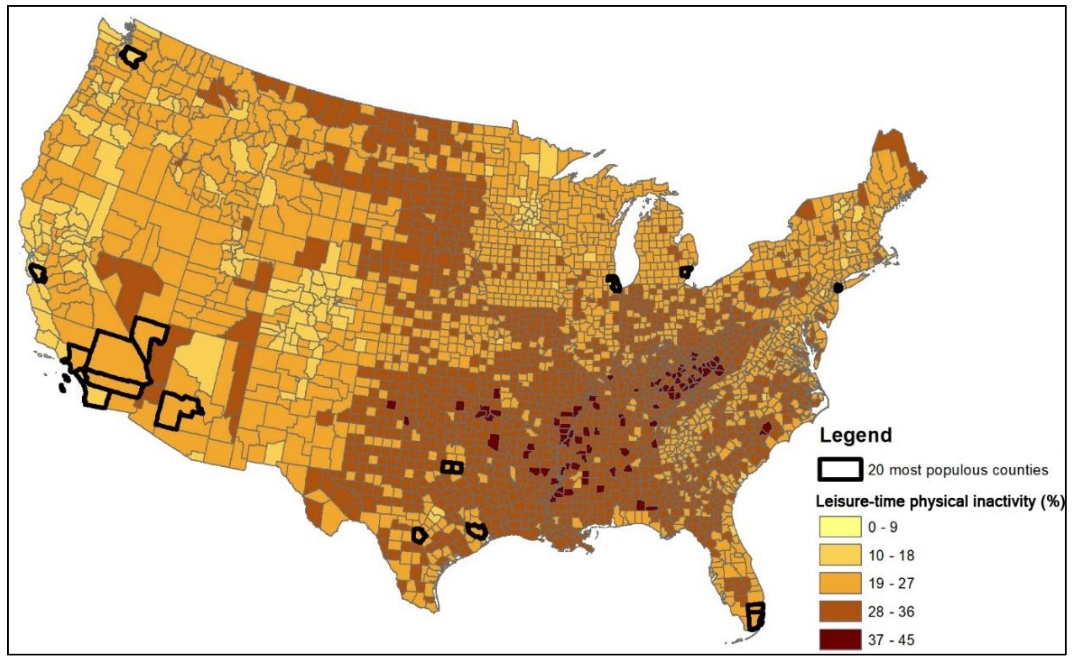
The physical inactivity data used in this study were generated by a cooperative project between the Robert Wood Johnson Foundation and the University of Wisconsin Population Health Institute in 2011. It was collected by the Behavioral Risk Factor Surveillance System (BRFSS) of the Centers for Disease Control and Prevention (CDC) through telephone surveys. In this study, LTPI was measured as the percentage of adults aged 20 and over reporting insufficient leisure-time physical activity. Figure 1 visualizes the LTPI data and the spatial pattern of LTPI across the contiguous U.S. Among the 3109 counties of the 48 contiguous states in the U.S., 3108 counties are selected for statistical analysis. One county is excluded because its physical inactivity value is not available. As shown in the figure, lower percentages of LTPI are found in the western and north-eastern states, whereas higher percentages of LTPI are in the south-eastern region. For instance, Colorado and Minnesota have many counties with low levels of LTPI, while West Virginia and Tennessee have many counties with high levels of LTPI.
2.1.2. Physical Environmental Factors
As noted by the National Research Council and the Institute of Medicine [71], “the factors in the physical environment that are important to health include harmful substances, such as air pollution or proximity to toxic sites (the focus of classic environmental epidemiology); access to various health-related resources (e.g., healthy or unhealthy foods, recreational resources, medical care); and community design and the ‘built environment’ (e.g., land use, street connectivity, transportation systems).” Past research has identified various environmental factors that influence people’s physical inactivity. These include land-use mix, street length/connectivity, transport facilities, and parks and recreational facilities [27]. High land-use mix and high street length/connectivity within the residential neighborhood have been found to have a negative association with the physical inactivity of both adults and children [20,25,26,30,34,36,39,40,72]. It has been found that the quality or density of sidewalks, the number of bus lines, and walking and biking trails around the home location or within the residential community are also positively correlated with the active travels of adults and children [29,33,38,73,74]. Exposure to green space and recreational facilities in the residential neighborhood has negative associations with physical inactivity [23,24,32,33,35,37,38]. Regarding access to green spaces, some studies, however, indicate that there is no significant association between physical inactivity and green spaces [28,31]. As one of the environmental factors, weather may affect physical inactivity. However, previous studies have not found any significant association between physical inactivity and weather [22,47,48,75].
Among many physical environmental factors, this study focuses on temperature, precipitation, land use, green space, and walkability, which are widely considered as factors that may influence health behaviors. These five physical environmental factors are listed in Table 1. Annual average temperature and precipitation are calculated using the method developed by Schlenker and Roberts [76] based on the 2011 daily temperature, and precipitation data in the U.S. were derived from the U.S. Department of Agriculture’s official climatological data. The percentage of tree canopy cover is calculated using the 2011 tree canopy data of the U.S. Forest Service. The percentage of highly developed area for each county is abstracted from the multi-resolution land characteristics consortium. Walkability is calculated by dividing the length of minor roads (km) in a county by the area of the county (km2). The minor road density is used as a surrogate of walkability, which is consistent with the walkability measurement method introduced by Schlossberg [77]. The road network and street classification data are abstracted from the topologically-integrated geographic encoding and referencing (TIGER) database.
2.1.3. Social Environmental Factors
Besides physical environmental factors, demographic characteristics, and socioeconomic status are also important determinants of physical inactivity. Evidence from many studies shows that young adults and men have lower levels of physical inactivity than older adults and women [41,42,44,46,78]. Regarding ethnicity, studies found that African American women have a higher rate of physical inactivity than white women, and minority groups were also found to have a higher rate of physical inactivity than the white population [41,42,46,78]. Education and income have a negative correlation with physical inactivity, and adults in urban areas have a lower rate of physical inactivity than adults in rural areas [28,41,46,78]. Non-professional workers have a higher rate of physical inactivity than professional workers, whereas marital status shows mixed associations [45,46]. High levels of physical inactivity are also correlated with car ownership, home ownership, and high utilization of active travel (e.g., walking and biking) for commuting [28,43,79].
In this study, county-level demographic and socioeconomic characteristics are used to represent social environmental factors that influence LTPI. By adopting the sociodemographic variables used in previous studies, the factors used in this study include age, gender, race, income, unemployment rate, occupation, travel mode of commute trips, house ownership, and car ownership. They are extracted from the 2011 American Community Survey (ACS) data. ACS five-year estimates data were used because they provide relatively high precision of the estimates based on large sample size when compared to one-year and three-year estimates [80]. These variables are listed in Table 1. The five demographic variables are the median age, the percentage of females, and the percentages of different ethnic groups. The 10 socioeconomic status variables are per capita income, unemployment rate, occupations, commuting mode, house ownership, and vehicle ownership.
2.2. Statistical Analysis
2.2.1. Multicollinearity
To evaluate the multicollinearity among the 20 independent variables, correlations, and variable inflation factors (VIF) are investigated. In a regression model, multicollinearity exists when two or more independent variables have high correlations. Multicollinearity can cause unstable coefficient estimates and thus hinder the precise interpretation of the results. Correlations between all pairs of the independent variable are analyzed using Pearson correlation test (the correlation matrix is not shown). None of the pairs shows strong correlation (correlation coefficient > 0.7 or correlation coefficient < −0.7). For VIF, the common threshold VIF < 10 was used [81,82], and all 20 independent variables are found to have VIF values less than 10. Thus, there is no evidence for multicollinearity among the 20 independent variables, all of which are used for further investigation in this study.
2.2.2. Spatial Regression Models
The presence of spatial autocorrelation in LTPI across counties in the U.S. is examined using the global Moran’s I statistic. The first order Queen’s contiguity method was applied to define adjacent neighbors since the shapes and sizes of counties and states are irregular [83]. The Moran’s I obtained is 0.58, which is greater than the expected value −0.0003 (p < 0.001), indicating strong spatial autocorrelation where counties tend to exhibit similar percentages of LTPI as nearby counties. The positive z-score of 119.78 also suggests that similar percentages of county-level LTPI tend to be spatially clustered, which can be observed in Figure 1. However, studies concerning the association between LTPI prevalence and environmental factors have largely ignored how spatial autocorrelation may play an important role in the results, given that environmental factors can have varying effects on LTPI depending on geographic location (a phenomenon known as spatial non-stationarity).
To explore and address the issue of spatial non-stationarity and its effects of the analytical result, spatial regression models (SLM and GWR) are employed in this study to examine the associations between environmental factors and LTPI as a function of geographic location. The results are also compared to those obtained with the OLS. The OLS is a linear regression model, which estimates coefficients by minimizing the sum of squares of the errors of predicted results. The OLS is one of the most widely used methods in LTPI research for investigating the association between environmental factors and LTPI [36,38,39,84]. However, the OLS does not consider any spatial variables or deal with spatial effects (e.g., spatial autocorrelation).
As the global spatial model, spatial lag regression can control the level of spatial autocorrelation by adopting a lag variable for the spatial effect to estimate regression models. The equation of spatial lag regression models [85] is
where is the dependent variable; is the weighted dependent variables summed over Queen contiguity neighborhood ; is the coefficient of the spatial lag; are the coefficients of the independent variables; are the independent variables; and is the random error term.
Compared to the SLM with the spatial lag estimated by weighted values, GWR generates local regression models for each spatial unit (e.g., the county in this study) to deal with spatial autocorrelation. The estimated coefficients of the independent variables thus vary between spatial units and are determined using Gaussian bell curve. The equation for GWR models [86] is
where is the dependent variable at th observation (e.g., county in this study); is the coefficient of the independent variable at the th observation, calculated based on Gaussian bell curve function; represents the independent variable at the th observation; and is the random error term. GeoDa and the R software package are used to run the GWR model in this study.
3. Results
3.1. Descriptive Statistics
The characteristics of LTPI and contextual variables are reported in Table 2. The percentage of physically inactive residents ranges from 10% to 45% among different counties. The average percentage of physically inactive residents is 27.15%, with a standard deviation of 5.06%. In terms of physical environmental factors, the counties include areas from tropical (average daily temperature = 24.78 °C) to continental (average daily temperature = −0.09 °C) climate, and from densely forested areas (% tree canopy coverage = 92.25) to deserts (% tree canopy coverage = 0.02). Also, highly developed urban areas (% highly developed area = 48.42) and developed areas with low or medium intensity or rural areas (% highly developed area = 0) are included in these counties. Meanwhile, the socioeconomic status and demographic characteristics of the counties are diverse. For instance, unemployment rates vary from 0% to 18.4%, covering counties without any unemployment problem and counties with significant unemployment problems. Per capita incomes range from $7887 to $61,290, covering impoverished and affluent counties. Population compositions of the counties vary considerably regarding age, gender, and race (e.g., from white to African American-dominated counties; from youngsters to seniors-dominated counties). Vehicle ownership represents the percentage of families who do not own a vehicle. There are some counties in which all families have at least one automobile while there are some in which most of the families do not own any vehicle (78%). The great variation in LTPI, physical environment, socioeconomic status, and demographic characteristics among the counties across the contiguous U.S. provides rich information for a basic understanding of the contexts in different counties.
3.2. OLS Regression
As shown by the regression results listed in Table 3, the OLS regression model explain most of the variation ( = 0.606) in the dependent variable (county-level LTPI). According to the results, the positively correlated independent variables includes temperature (p < 0.001); precipitation (p < 0.001); Occupation 1, 2, 3 (p < 0.001); self-employed unpaid family workers (p < 0.001); vehicle ownership (p < 0.001); age (p < 0.001); being female (p < 0.001); and being African American (Race 1) (p < 0.001). While six other variables are negatively correlated with LTPI—tree canopy coverage (p < 0.001); unemployment rate (p < 0.001); commuting mode 2 (p < 0.001); income (p < 0.001); being Asian (Race 2) (p < 0.01); and being Hispanic and Latino (Race 3) (p < 0.001). As a global regression model, OSL estimates coefficients by globally minimizing the sum of squares of the errors of predicted results. The significant correlations found are universally applied without the consideration of any spatial variables or effects.
3.3. Spatial Regression
Comparing the three models, the results of Akaike information criterion (AIC) show that the two spatial regression models—SLM (AIC = 14,745; = 0.744) and GWR (AIC =13,415; = 0.856)—have better explanatory power than the OLS model (AIC = 16,063; = 0.608) for LTPI. The AIC and are measures of the relative quality of statistical models for a given dataset: the lower the AIC and the higher the value, the better fit of the model for the dataset. Furthermore, as to the two spatial regression models, the GWR model, with a lower AIC, works better than SLM. The results from the GWR model are shown in Table 4. The model fits the data well and explains most of the variation in the dependent variable according to the adjusted of 0.814. Its local values range from 0.54 to 0.96 as shown in Figure 2. The figure shows that most counties have high values of 0.68 or above, which indicates that the GWR model predicts LTPI accurately in these counties.
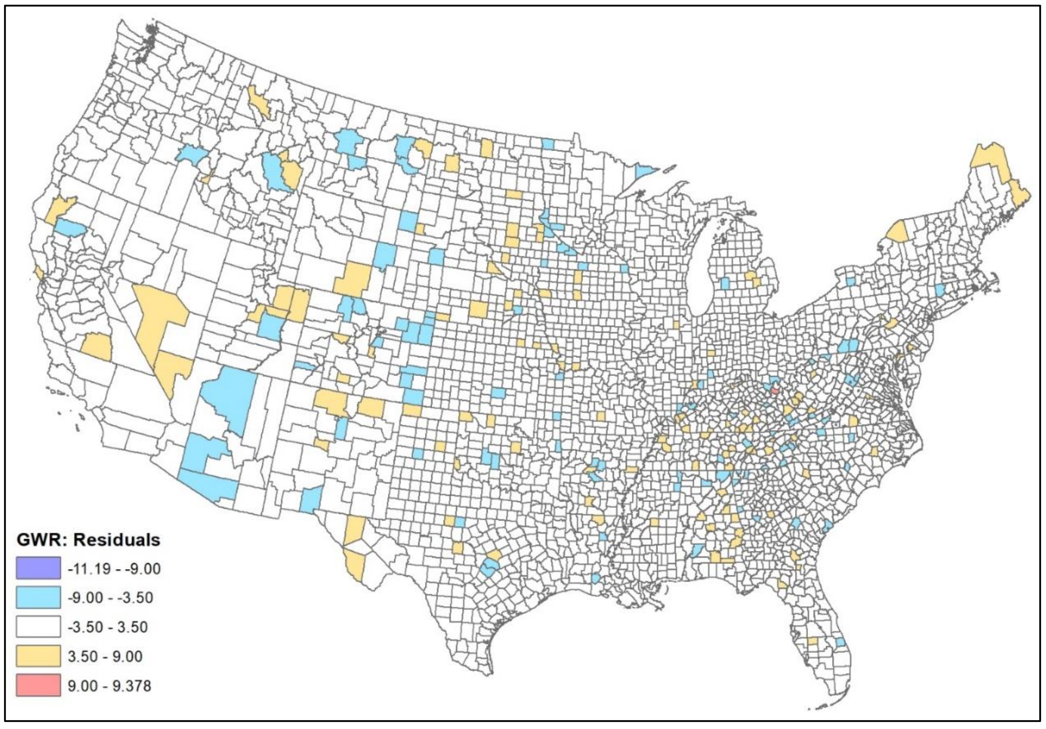
The residuals for both spatial models are visualized and shown in Figure 3 and Figure 4. In these two residual maps, positive residuals (red and yellow in the figures) indicate underestimated LTPI levels, and negative ones (purple and blue in the figures) indicate overestimated LTPI levels. As shown in the two figures, there is no significant spatial autocorrelation in the residual maps of the spatial lag regression model (Moran’s I = 0.0957) and the GWR model (Moran’s I = 0.0293).
In Table 4, the percentages of positive and negative coefficients, as well as the percentage of significant coefficient estimates, show that relevant environmental factors are mostly inconsistent regarding their associations across all counties. The columns of significant positive coefficient estimates (%) and significant negative coefficient estimates (%) indicate the percentage of the positive and negative coefficient estimates that are statistically significant, while the column of the significant coefficient estimates (%) shows the percentage of significant coefficient estimates among all counties based on the corresponding t-values (|t-value| ≥ 2.00). Given the coefficients for two of the variables are significant only in 30–50% of the counties, and that for most of the counties these coefficients are not different from zero (have no effect), we have to interpret the results carefully. For instance, if a coefficient’s t-value is not significant, the common advice is that it should not be interpreted it at all because we cannot be sure that the value of the corresponding parameter in the underlying regression model is not really zero. In light of this caveat, we discuss the results of the local regression models as follows.
Based on the t-values, for the self-employed unpaid family workers (β12), only 9% of the counties have significant associations. In addition, precipitation (β2), land cover (β4), commuting mode-1 (β7), occupation-1 (β9), and house ownership (β14) have low percentages of counties (smaller than 30%) with statistically significant associations. On the contrary, income (β13) has a strong consistent negative association between income and LTPI (i.e., poor people tend to be less active) in 98% (86% of them are statistically significant) of U.S. counties. The temperature (β1) and race-3 (β20) are also crucial factors, whose coefficients are significant for 60% and 56% of all the counties respectively. All the other variables have fair percentages of significant coefficient estimates. Among them, considering only the significant coefficients, Occupation 2 (β10) show fairly consistent positive associations with LTPI, while being Hispanic and Latino (β20) indicates fairly consistent negative correlations with LTPI. Other variables present inconsistent relationships.
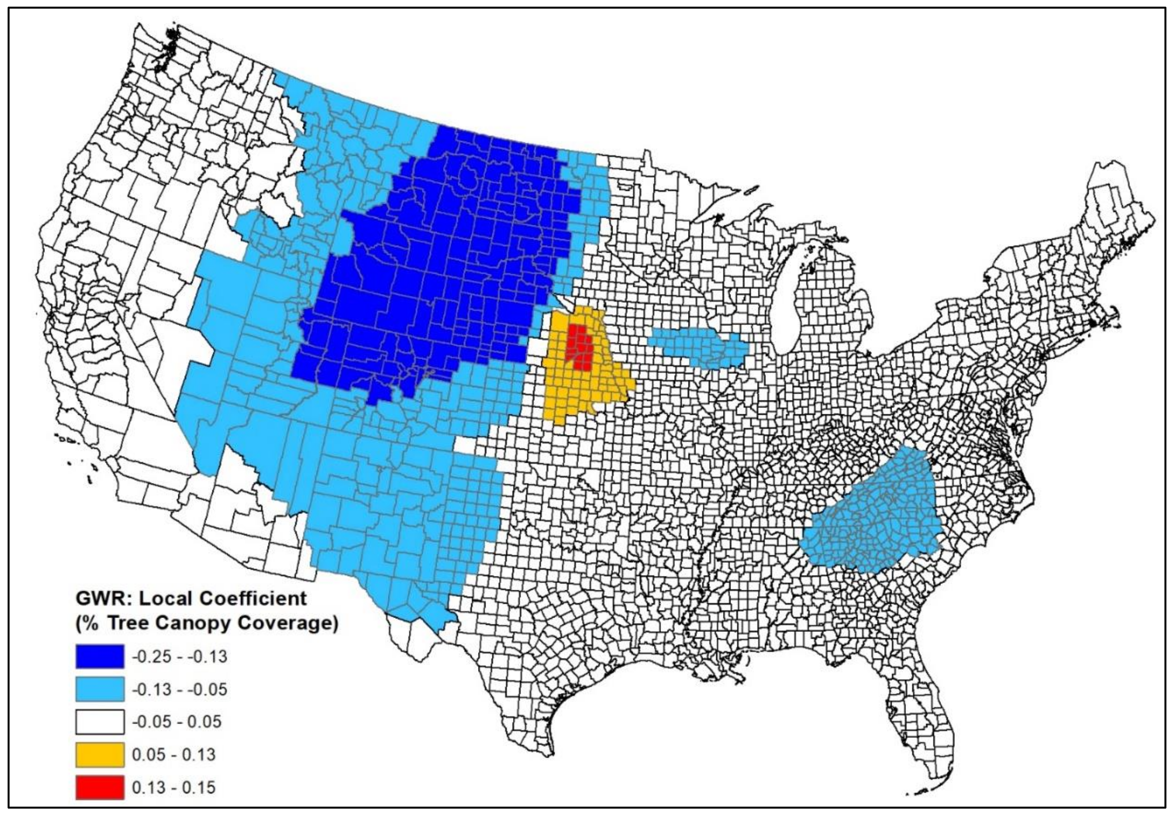
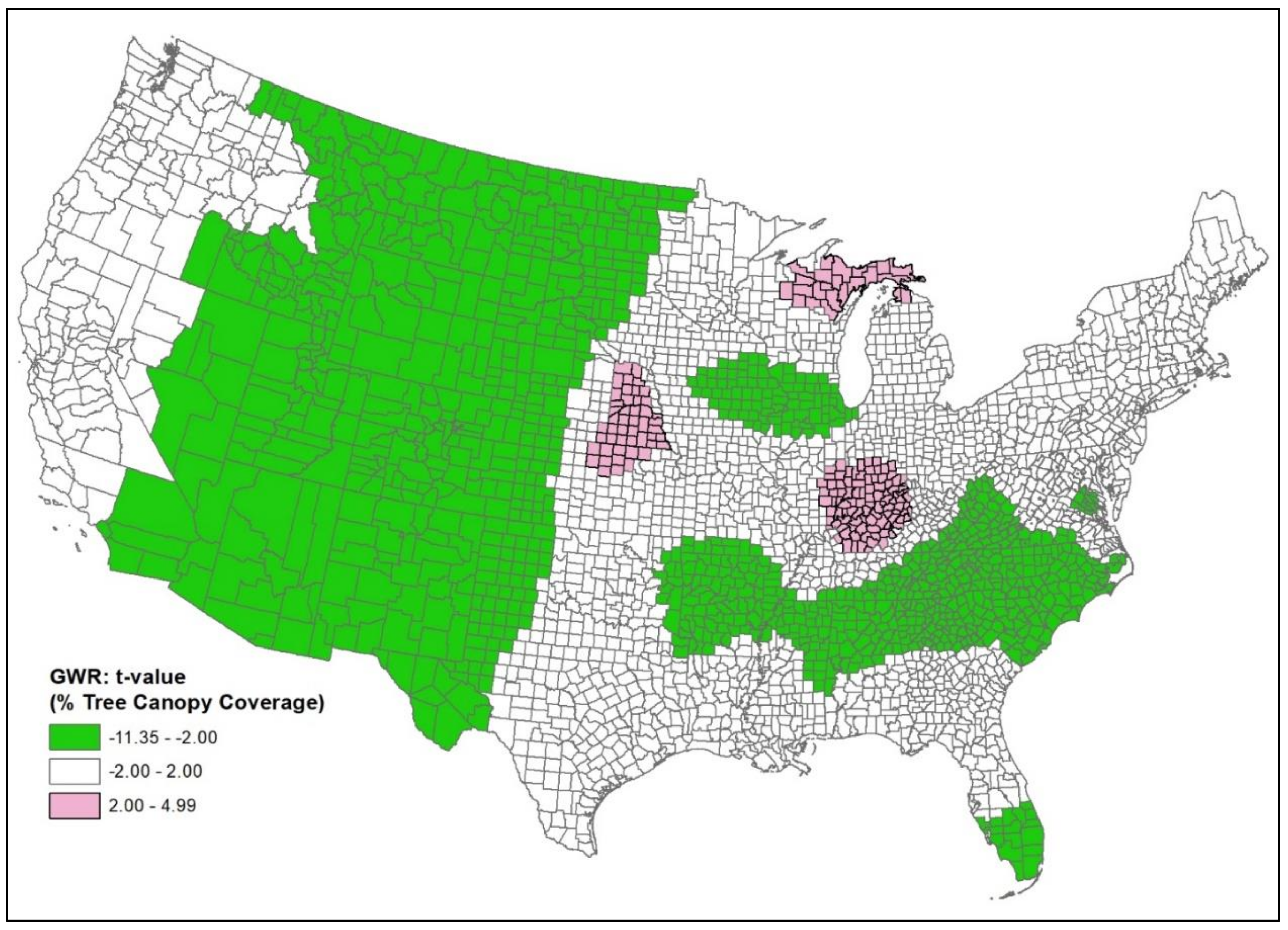
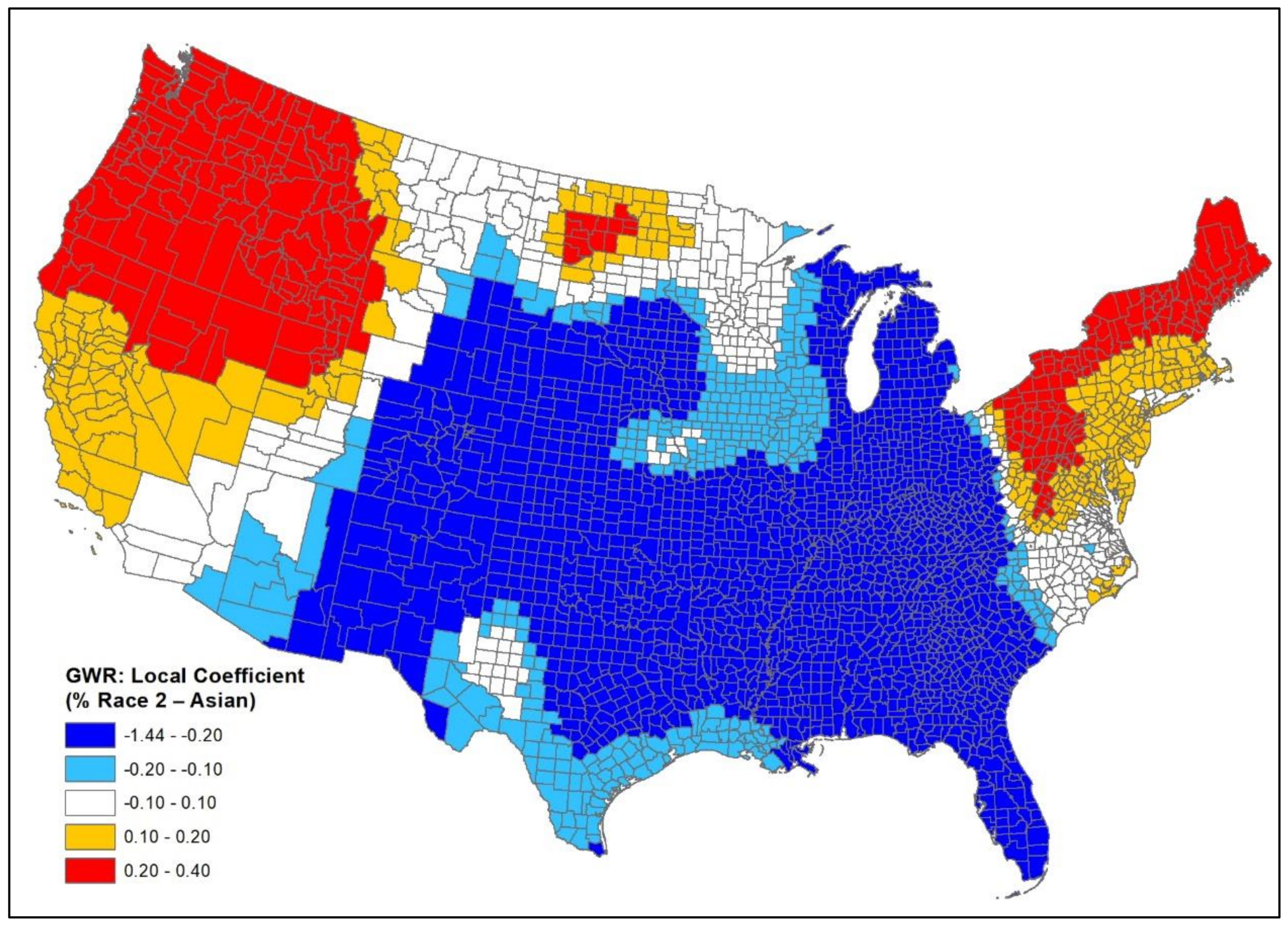
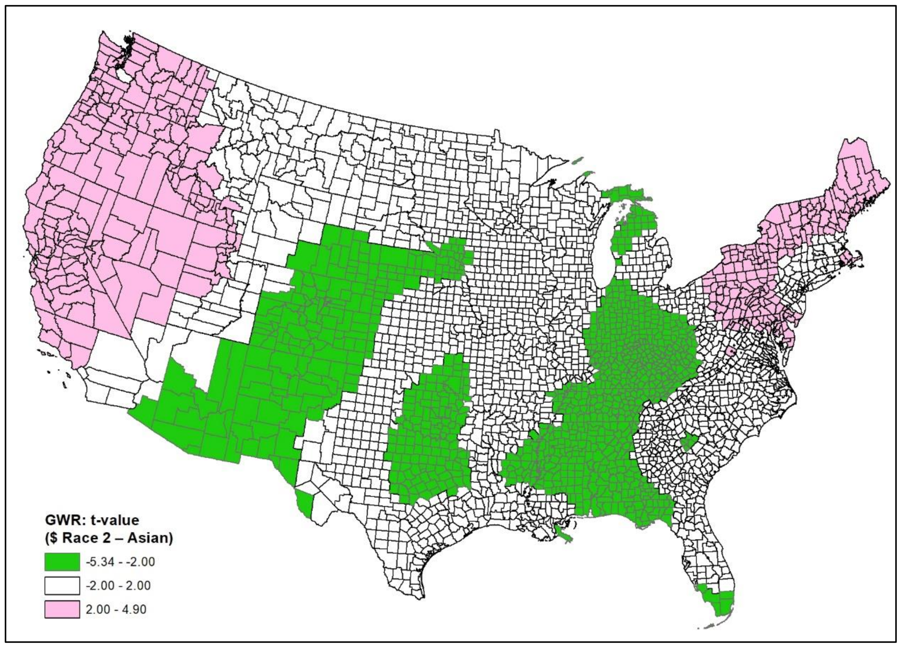
With the relatively inconsistent results concerning the environmental correlates of LTPI, we find evidence of spatial non-stationarity. Tree canopy coverage (β3) and Race 2 (β19) are chosen as two examples to illustrate the existence of spatial non-stationarity in the relationships between LTPI and environmental factors. Except for the GWR local coefficient for these two variables, the corresponding t-values are also mapped because the t-values help readers to effectively interpret the geographic distribution of the parameter estimates as well as their significance [87]. As shown in Figure 5 and Figure 6, the association between tree canopy coverage (β3) and LTPI fluctuates from negative (blue in Figure 5) to positive (red in Figure 5), with t-values (40% of them are statistically significant) illustrated in Figure 6. It can be seen that most counties have a significant negative association while some have a significant positive association. All the other counties do not have any significant correlation as indicated by the t-values. Figure 7 illustrates that the association between race-2 (β19) and LTPI also varies from negative (blue in Figure 7; 39% of them are statistically significant) to positive (red in Figure 7; 47% of them are statistically significant) while others do not have any significant association as indicated by the t-values illustrated in Figure 8. It can be seen from these figures that the counties with large positive and negative coefficients are statistically significant (as revealed by the t-values). These variations indicate that the relationships between environmental correlates and LTPI at the county level are spatially non-stationary.
We further investigate four selected coefficient estimates—tree canopy coverage (β3), walkability (β5), income (β13), and race-2 (β19)—of the GWR model for the 20 most populous U.S. counties (see Table 5). Most big cities are located in these 20 counties (bold polygons in Figure 1), which LTPI researchers may be interested in. The shaded coefficients in the table are statistically significant (|t-value| ≥ 2.00). The values of the 20 local models are high, ranging from 0.702 to 0.962. Income (β13) consistently shows a significant negative association with LTPI in the 20 counties. Note that the coefficients and 95% CI for income (β13) are close to zero because it has large values (ranging from 7887 to 61,290). Tree canopy coverage (β3) consistently shows a significant negative association with LTPI in 9 out of the 20 counties, while the other half of the counties do not have significant coefficients. Also, the walkability (β5) and Race 2 (β19) have mixed associations. As further demonstrated in Table 6, in the 20 most populous U.S. counties, no significant correlation is found for Commuting Mode 1 (β7) and Occupation 1 (β9). Also, different from the results of all counties, only temperature (β1), walkability (β5), unemployment rate (β6), age (β16), and Race 2 (β19) have inconsistent associations with LTPI while all the other contextual factors indicate relatively consistent associations.
4. Discussion and Conclusions
This study examined the effects of various contextual factors on LTPI at the county level in the contiguous U.S. The associations between these factors and LTPI were investigated using a non-spatial regression model (OSL) and two spatial regression models (SLM and GWR). By comparing the results of these three models, we found the existence of spatial autocorrelation and non-stationarity, which could lead to biased estimators but were mostly ignored in previous studies. While utilizing spatial regression models to address spatial autocorrelation, the inconsistent associations found between environmental factors and LTPI highlights the existence of spatial non-stationarity, which is another source of uncertainty for environmental health studies besides the MAUP and the UGCoP. The existence of spatial non-stationarity can partly explain the inconsistent findings in previous research conducted at different geographic locations. Also, the observed associations between environmental variables and LTPI are helpful for developing policies and interventions to create environmental settings that diminish LTPI at the county level.
As indicated by the result of the Moran’s I statistic, LTPI is spatially autocorrelated, which has rarely been considered in previous studies [13,21,41,70,88]. The lagged variable (Rho = 0.607) of SLM indicates the effect of the dependent variable in the neighbors on the dependent variable in the focal area. Neglecting the problems of spatial autocorrelation may lead to biased estimators and inaccurate results. Therefore, the spatial regression models, such as the SLM and GWR models, should be used in environmental health research. In this study, the spatial regression models perform better than the conventional OLS model based on the values of AIC and Log likelihood listed in Table 3 and Table 4. As indicated in Figure 3 and Figure 4, the low values of Moran’s I (SLM: 0.0957; GWR: 0.0293) in the residual maps suggest that the two spatial regression models handled the spatial autocorrelation in LTPI across different counties well and there is no systematic error in the models. The results also indicate that the performance of the GWR is better than the SLM in several ways. The Moran’s I of the SLM (0.0957) is larger than the Moran’s I of the GWR (0.0293), indicating that the GWR model may provide better predictions than the spatial lag model. Note that the Akaike information criterion (AIC) of the GWR model is 13,415, which is lower than the one of SLM (AIC = 14,745). These results corroborate the findings in previous research that GWR outperformed the spatial lag model in its explanatory power and predictive accuracy [89].
In addition, variations in the associations between environmental factors and LTPI across counties indicate the existence of spatial non-stationarity in such relationships, which has largely been ignored in previous research [13,70]. Different from conventional OLS and SLM regression models, the coefficient estimates of the environmental factors in the GWR show inconsistent results as indicated in Table 4. The results of the GWR model with t-values could help to investigate the various effects of environmental factors at different geographic locations. That is, one contextual factor can have statistically positive or negative coefficients (|t-value| ≥ 2.00) or no correlation (|t-value| < 2.00) depending on geographic location, which can be justified by the results from the local models. For instance, tree canopy coverage (β3) is significantly positively associated with LTPI for about 6% of the counties and negatively associated with LTPI for another 34% of the counties, while there is no significant association in the rest of the counties (60%). Figure 5 and Figure 6 visually reveal that its associations with LTPI fluctuate from negative (blue colored polygons) to positive (red colored polygons) and the corresponding t-value of each county. As shown in the figures, most of the western counties in states like Idaho, Nevada, Arizona, Utah, and Colorado have significantly negative coefficients, which means the percentage of tree canopy coverage is negatively associated with LTPI. In other words, the higher the percentage of tree canopy coverage, the lower the LTPI level. It is highly possible that these counties are mostly located in the semiarid and desert area with a lack of trees and green spaces, and thus tree canopy coverage may work more than expected to decrease LTPI. This finding also supports the empirical evidence of negative associations between tree canopy and LTPI in previous research [90,91,92]. On the other hand, tree canopy coverage (β3) in 6% of the counties has a positive association, and in 60% of the counties, it is not associated with LTPI, which does not correspond to the expected association. This finding may be interpreted in different perspectives considering the complicated interactions of LTPI with other environmental factors. Another example is Race 2 (β19), which is positively associated with LTPI in 11% of the counties while negatively associated with LTPI in 30% of the counties, and there is no significant association found in the other 59% of the counties. The distribution of the coefficients between Race 2 and LTPI as well as the t-values are illustrated in Figure 7 and Figure 8. It can be seen from the figures that there is a general pattern that in the western and northeastern counties, there are significantly positive relationships, while the relationship is significant and negative in the central and southern counties. These mixed results indicate that the relationships between environmental factors and LTPI at the county level are spatially non-stationary. Due to spatial non-stationarity, the direction of the association between environmental factors and LTPI varies by geographic location, which cannot be explained by classical ‘global’ models. Thus, the research findings at one location may not be generalized and applied globally. From the perspective of health policy, an effective policy that helps to decrease LTPI and promotes public health in one county may not be effective in another place due to spatial non-stationarity.
Different from the inconsistent associations found across all U.S. counties, some environmental factors show consistent associations with LTPI in the 20 most populous counties if not considering the non-significant estimates. For instance, tree canopy coverage (β3) has both positive and negative associations with LTPI as discussed above across all counties in the U.S., while it is only found to have significant negative coefficient estimates (see Table 5). Without surprise, the most populous counties usually are densely developed areas, and higher tree canopy coverage provides residents with more physical-activity-friendly spaces (e.g., parks) and therefore helps to decrease LTPI. In addition, as illustrated in Table 6, considering only the statistically significant estimates, contextual factors—such as Commuting 2 (β8), Occupation 2 (β10), and Occupation 3 (β11)—are all found to have consistent associations with LTPI in the 20 most populous counties while they are inconsistent across all counties in the U.S. (see Table 4). That means, due to the differences between rural and urban areas, there is a likelihood that environmental covariates can have consistent associations with LTPI in big cities despite the fact that they are inconsistently associated with LTPI across all counties in the U.S. Another interesting finding is the significant positive associations between walkability (β5) and LTPI in the northeastern counties (e.g., Queens, New York, and Kings), while walkability is negatively associated with LTPI in western and southeastern U.S. counties (e.g., Los Angeles, Clark, Miami-Dade, and Broward), and there is no significant relationships between them for all the other counties. It may be because of potential differences in culture and social structure among different areas of the U.S. Nonetheless, the reasons for the contrary associations are not clear, and further investigation is needed.
Consistent with expectations but in contrast to most previous studies, the findings of this study indicate the existence of spatial non-stationarity in environmental health studies. Thus, it is possible and not surprising that two similar studies concerning the effects of the same environmental factor on LTPI would observe inverse associations if they are conducted in different regions of the country. This is perhaps one of the reasons why research findings were often inconsistent concerning the effects of environmental factors on health behaviors and outcomes, given that past studies on the same issue (e.g., LTPI) were often conducted in different geographic locations (e.g., [93,94]). The assessment of spatial non-stationarity and the varying environmental effects on LTPI as a function of geographic location may help us investigate and better understand how space plays a role in the prevalence of LTPI across space [95].
This study found the location-based relationships between LTPI and different environmental, socio-economic, and demographic variables. These variables will be helpful for developing location-based policies and intervention measures that aim at decreasing LTPI and promoting health. For instance, communities in high-temperature and high-precipitation areas should provide more indoor physical activity facilities instead of outdoor facilities. Intervention policies that target social groups with higher levels of LTPI (e.g., women and African Americans) should be developed to encourage them to increase their physical activity levels. Also, in light of the negative association between tree canopy coverage and LTPI in urban areas, constructing more green spaces or parks in densely developed areas will be helpful for encouraging more physical activity. Other possible policies include promoting the use of active transport (e.g., walking), more flexible work schedules, and provision of more indoor physical activity facilities in densely developed areas.
This research has several limitations that need to be addressed in future studies. First, although 20 contextual factors are selected for the analysis, other contextual factors may also influence LTPI. Therefore, more contextual variables need to be considered and explored in future studies. For instance, more physical environmental variables can be included in the model, such as road network connectivity, the quality and density of sidewalks, the number of bus lines, and the length of walking and biking trails. Furthermore, this study used tree canopy coverage as a proxy for assessing the overall accessibility of green spaces in a county to its residents: the more green space a country has, the easier its residents can access parks and green spaces. However, future studies should consider measuring accessibility to green space more directly and including it to the models. Second, as an exploration of spatial non-stationarity, this study did not consider NLTPI, which has also shown to be associated with specific environmental factors. Further analysis of NLTPI is needed to understand the effects of environmental factors on physical inactivity comprehensively. Third, this is a cross-sectional study that used LTPI and environmental data only for the year 2011. Longitudinal analysis based on multi-year data may provide further insights into the effects of many environmental factors on people’s physical inactivity. Lastly, this study explored the inconsistent associations between LTPI and environmental factors at the county level to illustrate the existence of spatial non-stationarity and its influence on the results, which is underexplored. Spatial non-stationarity and its influence on the results may be different at various spatial scales. Thus, further investigation on how geographic scale may affect spatial non-stationarity is needed. Explorations of the effects of the MAUP (e.g., scale effects) and the UGCoP on the inconsistent results are outside the scope of this paper. Future study needs to thoroughly investigate all these three sources of contextual uncertainty through experiments conducted at different spatial scales with varying methods of measurement in environmental health studies (e.g., [96,97,98]).
This study highlights the existence of spatial non-stationarity and the importance of spatial regression model in environmental health studies. It provides useful insights into the environmental influences on health behaviors, such as LTPI. Since spatial autocorrelation and spatial non-stationarity are often present in public health data, they should be addressed seriously to generate reliable results. LTPI is and will continue to be one of the most critical public health concerns in the U.S., the knowledge generated from this study will assist community health professionals, city planners, and government decision-makers in diminishing LTPI and mitigating the rise of inactivity-related chronic disease.
Acknowledgments
The authors would like to thank the three anonymous reviewers for their valuable comments on the manuscript.
Author Contributions
J.W. and K.L. conceived, designed and implemented the experiments; J.W. analyzed the results and wrote the paper with K.L.; M.-P.K. contributed to refining and revising the paper.
Conflicts of Interest
The authors declare no conflict of interest.
References
- Berke, E.M.; Koepsell, T.D.; Moudon, A.V.; Hoskins, R.E.; Larson, E.B. Association of the built environment with physical activity and obesity in older persons. Am. J. Public Health 2007, 97, 486–492. [Google Scholar] [CrossRef] [PubMed]
- Duvall, J.; Sullivan, W.C. How to get more out of the green exercise experience. In Green Exercise Linking Nature, Health and Well-Being; Routledge: Abingdon, UK, 2016; Volume 37. [Google Scholar]
- Mitchell, R.; Popham, F. Effect of exposure to natural environment on health inequalities: An observational population study. Lancet 2008, 372, 1655–1660. [Google Scholar] [CrossRef]
- Stigsdotter, U.K.; Ekholm, O.; Schipperijn, J.; Toftager, M.; Kamper-Jorgensen, F.; Randrup, T.B. Health promoting outdoor environments-Associations between green space, and health, health-related quality of life and stress based on a Danish national representative survey. Scand. J. Soc. Med. 2010, 38, 411–417. [Google Scholar] [CrossRef] [PubMed]
- Macintyre, S.; Ellaway, A.; Cummins, S. Place effects on health: How can we conseptualise, operationalise and measure them? Soc. Sci. Med. 2002, 55, 125–139. [Google Scholar] [CrossRef]
- Rodriguez, D.A.; Brown, A.L.; Troped, P.J. Portable global positioning units to complement accelerometry-based physical activity monitors. Med. Sci. Sports Exerc. 2005, 37, S572–S581. [Google Scholar] [CrossRef] [PubMed]
- Rodríguez, D.A.; Cho, G.-H.; Evenson, K.R.; Conway, T.L.; Cohen, D.; Ghosh-Dastidar, B.; Pickrel, J.L.; Veblen-Mortenson, S.; Lytle, L.A. Out and about: Association of the built environment with physical activity behaviors of adolescent females. Health Place 2012, 18, 55–62. [Google Scholar] [CrossRef] [PubMed]
- Wheeler, B.W.; Cooper, A.R.; Page, A.S.; Jago, R. Greenspace and children’s physical activity: A GPS/GIS analysis of the PEACH project. Prev. Med. 2010, 51, 148–152. [Google Scholar] [CrossRef] [PubMed]
- Arem, H.; Moore, S.C.; Patel, A.; Hartge, P.; Berrington De Gonzalez, A.; Visvanathan, K.; Campbell, P.T.; Freedman, M.; Weiderpass, E.; Adami, H.O.; et al. Leisure time physical activity and mortality: A detailed pooled analysis of the dose-response relationship. JAMA Intern. Med. 2015, 175, 959–967. [Google Scholar] [CrossRef] [PubMed]
- O’Donovan, G.; Lee, I.M.; Hamer, M.; Stamatakis, E. Association of “weekend warrior” and other leisure time physical activity patterns with risks for all-cause, cardiovascular disease, and cancer mortality. JAMA Intern. Med. 2017, 177, 335–342. [Google Scholar] [CrossRef] [PubMed]
- Lahti, J.; Holstila, A.; Lahelma, E.; Rahkonen, O. Leisure-time physical activity and all-cause mortality. PLoS ONE 2014, 9, e101548. [Google Scholar] [CrossRef] [PubMed]
- Moore, S.C.; Lee, I.M.; Weiderpass, E.; Campbell, P.T.; Sampson, J.N.; Kitahara, C.M.; Keadle, S.K.; Arem, H.; De Gonzalez, A.B.; Hartge, P.; et al. Association of leisure-time physical activity with risk of 26 types of cancer in 1.44 million adults. JAMA Intern. Med. 2016, 176, 816–825. [Google Scholar] [CrossRef] [PubMed]
- Ewing, R.; Schmid, T.; Killingsworth, R.; Zlot, A.; Raudenbush, S. Relationship between urban sprawl and physical activity, obesity, and morbidity. Am. J. Health Promot. 2003, 18, 47–57. [Google Scholar] [CrossRef] [PubMed]
- U.S. Department of Health and Human Services. Physical Activity and Health: A Report of the Surgeon General; U.S. Department of Health and Human Services: Atlanta, GA, USA, 1996.
- Neumark-Sztainer, D. Multicontextual correlates of adolescent leisure-time physical activity. Am. J. Prev. Med. 2014, 46, 605–616. [Google Scholar] [CrossRef]
- Sallis, J.F.; Owen, N.; Fisher, E. Ecological models of health behavior. In Health Behavior and Health Education: Theory, Research, and Practice; Jossey-Bass: San Francisco, CA, USA, 2015; Volume 5, pp. 43–64. [Google Scholar]
- Su, M.; Tan, Y.Y.; Liu, Q.M.; Ren, Y.J.; Kawachi, I.; Li, L.M.; Lv, J. Association between perceived urban built environment attributes and leisure-time physical activity among adults in Hangzhou, China. Prev. Med. 2014, 66, 60–64. [Google Scholar] [CrossRef] [PubMed]
- Adams, M.A.; Todd, M.; Kurka, J.; Conway, T.L.; Cain, K.L.; Frank, L.D.; Sallis, J.F. Patterns of Walkability, Transit, and Recreation Environment for Physical Activity. Am. J. Prev. Med. 2015, 49, 878–887. [Google Scholar] [CrossRef] [PubMed]
- Mitchell, C.A.; Clark, A.F.; Gilliland, J.A. Built environment influences of children’s physical activity: Examining differences by neighbourhood size and sex. Int. J. Environ. Res. Public Health 2016, 13, 130. [Google Scholar] [CrossRef] [PubMed]
- Roemmich, J.N.; Epstein, L.H.; Raja, S.; Yin, L. The neighborhood and home environments: Disparate relationships with physical activity and sedentary behaviors in youth. Ann. Behav. Med. 2007, 33, 29–38. [Google Scholar] [CrossRef] [PubMed]
- Gordon-Larsen, P.; Nelson, M.C.; Page, P.; Popkin, B.M. Inequality in the built environment underlies key health disparities in physical activity and obesity. Pediatrics 2006, 117, 417–424. [Google Scholar] [CrossRef] [PubMed]
- King, A.C.; Castro, C.; Wilcox, S.; Eyler, A.A.; Sallis, J.F.; Brownson, R.C. Personal and environmental factors associated with physical inactivity among different racial-ethnic groups of US middle-aged and older-aged women. Health Psychol. 2000, 19, 354–364. [Google Scholar] [CrossRef] [PubMed]
- Coombes, E.; Jones, A.P.; Hillsdon, M. The relationship of physical activity and overweight to objectively measured green space accessibility and use. Soc. Sci. Med. 2010, 70, 816–822. [Google Scholar] [CrossRef] [PubMed]
- Fisher, K.J.; Li, F.; Michael, Y.; Cleveland, M. Neighborhood-level influences on physical activity among older adults: A multilevel analysis. J. Aging Phys. Act. 2004, 12, 45–63. [Google Scholar] [CrossRef] [PubMed]
- Frank, L.; Kerr, J.; Chapman, J.; Sallis, J. Urban form relationships with walk trip frequency and distance among youth. Am. J. Health Promot. 2007, 21, 305–311. [Google Scholar] [CrossRef] [PubMed]
- Grow, H.; Saelens, B.; Kerr, J.; Durant, N.; Norman, G.; Sallis, J. Where are youth active? Roles of proximity, active transport, and built environment. Med. Sci. Sports Exerc. 2008, 40, 2071–2079. [Google Scholar] [CrossRef] [PubMed]
- Handy, S.L.; Boarnet, M.G.; Ewing, R.; Killingsworth, R.E. How the built environment affects physical activity: Views from urban planning. Am. J. Prev. Med. 2002, 23, 64–73. [Google Scholar] [CrossRef]
- Hillsdon, M.; Panter, J.; Foster, C.; Jones, A. The relationship between access and quality of urban green space with population physical activity. Public Health 2006, 120, 1127–1132. [Google Scholar] [CrossRef] [PubMed]
- Hoehner, C.M.; Ramirez, L.K.B.; Elliott, M.B.; Handy, S.L.; Brownson, R.C. Perceived and objective environmental measures and physical activity among urban adults. Am. J. Prev. Med. 2005, 28, 105–116. [Google Scholar] [CrossRef] [PubMed]
- Kerr, J.; Frank, L.; Sallis, J.F.; Chapman, J. Urban form correlates of pedestrian travel in youth: Differences by gender, race-ethnicity and household attributes. Transp. Res. Part D Transp. Environ. 2007, 12, 177–182. [Google Scholar] [CrossRef]
- Maas, J.; Verheij, R.A.; Spreeuwenberg, P.; Groenewegen, P.P. Physical activity as a possible mechanism behind the relationship between green space and health: A multilevel analysis. BMC Public Health 2008, 8, 206. [Google Scholar] [CrossRef] [PubMed]
- Mota, J.; Almeida, M.; Santos, P.; Ribeiro, J.C. Perceived neighborhood environments and physical activity in adolescents. Prev. Med. 2005, 41, 834–836. [Google Scholar] [CrossRef] [PubMed]
- Nagel, C.L.; Carlson, N.E.; Bosworth, M.; Michael, Y.L. The relation between neighborhood built environment and walking activity among older adults. Am. J. Epidemiol. 2008, 168, 461–468. [Google Scholar] [CrossRef] [PubMed]
- Saelens, B.E.; Sallis, J.F.; Black, J.B.; Chen, D. Neighborhood-based differences in physical activity: An environment scale evaluation. Am. J. Public Health 2003, 93, 1552–1558. [Google Scholar] [CrossRef] [PubMed]
- Sallis, J.F.; Bowles, H.R.; Bauman, A.; Ainsworth, B.E.; Bull, F.C.; Craig, C.L.; Sjöström, M.; De Bourdeaudhuij, I.; Lefevre, J.; Matsudo, V. Neighborhood environments and physical activity among adults in 11 countries. Am. J. Prev. Med. 2009, 36, 484–490. [Google Scholar] [CrossRef] [PubMed]
- Sallis, J.F.; Cerin, E.; Conway, T.L.; Adams, M.A.; Frank, L.D.; Pratt, M.; Salvo, D.; Schipperijn, J.; Smith, G.; Cain, K.L.; et al. Physical activity in relation to urban environments in 14 cities worldwide: A cross-sectional study. Lancet 2016, 387, 2207–2217. [Google Scholar] [CrossRef]
- Santos, M.P.; Page, A.S.; Cooper, A.R.; Ribeiro, J.C.; Mota, J. Perceptions of the built environment in relation to physical activity in Portuguese adolescents. Health Place 2009, 15, 548–552. [Google Scholar] [CrossRef] [PubMed]
- Troped, P.J.; Saunders, R.P.; Pate, R.R.; Reininger, B.; Addy, C.L. Correlates of recreational and transportation physical activity among adults in a New England community. Prev. Med. 2003, 37, 304–310. [Google Scholar] [CrossRef]
- Troped, P.J.; Wilson, J.S.; Matthews, C.E.; Cromley, E.K.; Melly, S.J. The Built Environment and Location-Based Physical Activity. Am. J. Prev. Med. 2010, 38, 429–438. [Google Scholar] [CrossRef] [PubMed]
- Browning, M.; Lee, K. Within what distance does “Greenness” best predict physical health? A systematic review of articles with GIS buffer analyses across the lifespan. Int. J. Environ. Res. Public Health 2017, 14, 675. [Google Scholar] [CrossRef] [PubMed]
- Brown, D.W.; Balluz, L.S.; Heath, G.W.; Moriarty, D.G.; Ford, E.S.; Giles, W.H.; Mokdad, A.H. Associations between recommended levels of physical activity and health-related quality of life Findings from the 2001 Behavioral Risk Factor Surveillance System (BRFSS) survey. Prev. Med. 2003, 37, 520–528. [Google Scholar] [CrossRef]
- Fontaine, K.R.; Heo, M.; Bathon, J. Are US adults with arthritis meeting public health recommendations for physical activity? Arthritis Rheum. 2004, 50, 624–628. [Google Scholar] [CrossRef] [PubMed]
- Gordon-Larsen, P.; Nelson, M.C.; Beam, K. Associations among active transportation, physical activity, and weight status in young adults. Obes. Res. 2005, 13, 868–875. [Google Scholar] [CrossRef] [PubMed]
- Jones, A.P.; Coombes, E.G.; Griffin, S.J.; van Sluijs, E.M. Environmental supportiveness for physical activity in English schoolchildren: A study using Global Positioning Systems. Int. J. Behav. Nutr. Phys. Act. 2009, 6, 42. [Google Scholar] [CrossRef] [PubMed]
- Salmon, J.; Owen, N.; Bauman, A.; Schmitz, M.K.H.; Booth, M. Leisure-time, occupational, and household physical activity among professional, skilled, and less-skilled workers and homemakers. Prev. Med. 2000, 30, 191–199. [Google Scholar] [CrossRef] [PubMed]
- Trost, S.G.; Owen, N.; Bauman, A.E.; Sallis, J.F.; Brown, W. Correlates of adults’ participation in physical activity: Review and update. Med. Sci. Sports Exerc. 2002, 34, 1996–2001. [Google Scholar] [CrossRef] [PubMed]
- Sallis, J.; Bauman, A.; Pratt, M. Environmental and policy interventions to promote physical activity. Am. J. Prev. Med. 1998, 15, 379–397. [Google Scholar] [CrossRef]
- Sallis, J.F.; Cervero, R.B.; Ascher, W.; Henderson, K.A.; Kraft, M.K.; Kerr, J. An ecological approach to creating active living communities. Annu. Rev. Public Health 2006, 27, 297–322. [Google Scholar] [CrossRef] [PubMed]
- Jago, R.; Baranowski, T.; Baranowski, J.C. Observed, GIS, and self-reported environmental features and adolescent physical activity. Am. J. Health Promot. 2006, 20, 422–428. [Google Scholar] [CrossRef] [PubMed]
- Roemmich, J.N.; Epstein, L.H.; Raja, S.; Yin, L.; Robinson, J.; Winiewicz, D. Association of access to parks and recreational facilities with the physical activity of young children. Prev. Med. 2006, 43, 437–441. [Google Scholar] [CrossRef] [PubMed]
- Jago, R.; Baranowski, T.; Harris, M. Relationships between GIS environmental features and adolescent male physical activity: GIS coding differences. J. Phys. Act. Health 2006, 3, 230–242. [Google Scholar] [CrossRef] [PubMed]
- Tucker, P.; Irwin, J.D.; Gilliland, J.; He, M.; Larsen, K.; Hess, P. Environmental influences on physical activity levels in youth. Health Place 2009, 15, 357–363. [Google Scholar] [CrossRef] [PubMed]
- Cohen, D.A.; Ashwood, J.S.; Scott, M.M.; Overton, A.; Evenson, K.R.; Staten, L.K.; Porter, D.; McKenzie, T.L.; Catellier, D. Public parks and physical activity among adolescent girls. Pediatrics 2006, 118, 1381–1389. [Google Scholar] [CrossRef] [PubMed]
- Dowda, M.; Brown, W.H.; McIver, K.L.; Pfeiffer, K.A.; O’Neill, J.R.; Addy, C.L.; Pate, R.R. Policies and characteristics of the preschool environment and physical activity of young children. Pediatrics 2009, 123, e261–e266. [Google Scholar] [CrossRef] [PubMed]
- Timperio, A.; Giles-Corti, B.; Crawford, D.; Andrianopoulos, N.; Ball, K.; Salmon, J.; Hume, C. Features of public open spaces and physical activity among children: Findings from the CLAN study. Prev. Med. 2008, 47, 514–518. [Google Scholar] [CrossRef] [PubMed]
- Kerr, J.; Norman, G.J.; Sallis, J.F.; Patrick, K. Exercise aids, neighborhood safety, and physical activity in adolescents and parents. Med. Sci. Sports Exerc. 2008, 40, 1244–1248. [Google Scholar] [CrossRef] [PubMed]
- Carver, A.; Timperio, A.F.; Crawford, D.A. Neighborhood road environments and physical activity among youth: The CLAN study. J. Urban Health 2008, 85, 532–544. [Google Scholar] [CrossRef] [PubMed]
- Braza, M.; Shoemaker, W.; Seeley, A. Neighborhood design and rates of walking and biking to elementary school in 34 California communities. Am. J. Health Promot. 2004, 19, 128–136. [Google Scholar] [CrossRef] [PubMed]
- Larsen, K.; Gilliland, J.; Hess, P.; Tucker, P.; Irwin, J.; He, M. The influence of the physical environment and sociodemographic characteristics on children’s mode of travel to and from school. Am. J. Public Health 2009, 99, 520–526. [Google Scholar] [CrossRef] [PubMed]
- Houston, D. Implications of the modifiable areal unit problem for assessing built environment correlates of moderate and vigorous physical activity. Appl. Geogr. 2014, 50, 40–47. [Google Scholar] [CrossRef]
- Lovasi, G.S.; Grady, S.; Rundle, A. Steps Forward: Review and Recommendations for Research on Walkability, Physical Activity and Cardiovascular Health. Public Health Rev. 2012, 33, 484–506. [Google Scholar] [CrossRef] [PubMed]
- Koohsari, M.J.; Badland, H.; Giles-Corti, B. (Re)Designing the built environment to support physical activity: Bringing public health back into urban design and planning. Cities 2013, 35, 294–298. [Google Scholar] [CrossRef]
- Dunton, G.F.; Almanza, E.; Jerrett, M.; Wolch, J.; Pentz, M.A. Neighborhood park use by children: Use of accelerometry and global positioning systems. Am. J. Prev. Med. 2014, 46, 136–142. [Google Scholar] [CrossRef] [PubMed]
- Liao, Y.; Intille, S.S.; Dunton, G.F. Using ecological momentary assessment to understand where and with whom adults’ physical and sedentary activity occur. Int. J. Behav. Med. 2015, 22, 51–61. [Google Scholar] [CrossRef] [PubMed]
- Schwanen, T.; Wang, D. Well-Being, Context, and Everyday Activities in Space and Time. Ann. Assoc. Am. Geogr. 2014, 104, 833–851. [Google Scholar] [CrossRef]
- Buck, C.; Kneib, T.; Tkaczick, T.; Konstabel, K.; Pigeot, I. Assessing opportunities for physical activity in the built environment of children: Interrelation between kernel density and neighborhood scale. Int. J. Health Geogr. 2015, 14, 35. [Google Scholar] [CrossRef] [PubMed]
- Kwan, M. The Uncertain Geographic Context Problem. Ann. Assoc. Am. Geogr. 2012, 102, 958–968. [Google Scholar] [CrossRef]
- Kwan, M. How GIS can help address the uncertain geographic context problem in social science research. Ann. GIS 2012, 18, 245–255. [Google Scholar] [CrossRef]
- Bish, C.L.; Blanck, H.M.; Serdula, M.K.; Marcus, M.; Kohl, H.W.; Khan, L.K. Diet and physical activity behaviors among Americans trying to lose weight: 2000 Behavioral Risk Factor Surveillance System. Obes. Res. 2005, 13, 596–607. [Google Scholar] [CrossRef] [PubMed]
- Ewing, R.; Meakins, G.; Hamidi, S.; Nelson, A.C. Relationship between urban sprawl and physical activity, obesity, and morbidity-Update and refinement. Health Place 2014, 26, 118–126. [Google Scholar] [CrossRef] [PubMed]
- Council, N.R.; Population, C. US Health in International Perspective: Shorter Lives, Poorer Health; Woolf, S.H., Aron, L., Eds.; National Academies Press: Washington, DC, USA, 2013; ISBN 0309264146. [Google Scholar]
- Ding, D.; Sallis, J.F.; Kerr, J.; Lee, S.; Rosenberg, D.E. Neighborhood environment and physical activity among youth: A review. Am. J. Prev. Med. 2011, 41, 442–455. [Google Scholar] [CrossRef] [PubMed]
- Brownson, R.C.; Housemann, R.A.; Brown, D.R.; Jackson-Thompson, J.; King, A.C.; Malone, B.R.; Sallis, J.F. Promoting physical activity in rural communities: Walking trail access, use, and effects. Am. J. Prev. Med. 2000, 18, 235–241. [Google Scholar] [CrossRef]
- Troped, P.J.; Saunders, R.P.; Pate, R.R.; Reininger, B.; Ureda, J.R.; Thompson, S.J. Associations between self-reported and objective physical environmental factors and use of a community rail-trail. Prev. Med. 2001, 32, 191–200. [Google Scholar] [CrossRef] [PubMed]
- Sallis, J.F.; Hovell, M.F.; Hofstetter, C.R.; Faucher, P.; Elder, J.P.; Blanchard, J.; Caspersen, C.J.; Powell, K.E.; Christenson, G.M. A multivariate study of determinants of vigorous exercise in a community sample. Prev. Med. 1989, 18, 20–34. [Google Scholar] [CrossRef]
- Schlenker, W.; Roberts, M.J. Nonlinear temperature effects indicate severe damages to US crop yields under climate change. Proc. Natl. Acad. Sci. USA 2009, 106, 15594–15598. [Google Scholar] [CrossRef] [PubMed]
- Schlossberg, M. From TIGER to Audit Instruments: Measuring Neighborhood Walkability with Street Data Based on Geographic Information Systems. Transp. Res. Rec. 2006, 1982, 48–56. [Google Scholar] [CrossRef]
- Sallis, J.F.; Simons-Morton, B.G.; Stone, E.J.; Corbin, C.B.; Epstein, L.H.; Faucette, N.; Iannotti, R.J.; Killen, J.D.; Klesges, R.C.; Petray, C.K.; et al. Determinants of physical activity and interventions in youth. Med. Sci. Sport. Exerc. 1992, 24, S248–S257. [Google Scholar] [CrossRef]
- Ahmed, N.U.; Smith, G.L.; Flores, A.M.; Pamies, R.J.; Mason, H.R.; Woods, K.F.; Stain, S.C. Racial/ethnic disparity and predictors of leisure-time physical activity among US men. Ethn. Dis. 2005, 15, 40–52. [Google Scholar] [PubMed]
- U.S. Census Bureau. A Compass for Understanding and Using What General Data: What Researchers Need to Know; U.S. Census Bureau: Washington, DC, USA, 2009.
- Lin, C.H.; Wen, T.H. Using geographically weighted regression (GWR) to explore spatial varying relationships of immature mosquitoes and human densities with the incidence of dengue. Int. J. Environ. Res. Public Health 2011, 8, 2798–2815. [Google Scholar] [CrossRef] [PubMed]
- O’brien, R.M. A caution regarding rules of thumb for variance inflation factors. Qual. Quant. 2007, 41, 673–690. [Google Scholar] [CrossRef]
- Tsai, P.-J.; Lin, M.-L.; Chu, C.-M.; Perng, C.-H. Spatial autocorrelation analysis of health care hotspots in Taiwan in 2006. BMC Public Health 2009, 9, 464. [Google Scholar] [CrossRef] [PubMed]
- Jansen, M.; Ettema, D.; Pierik, F.; Dijst, M. Sports facilities, shopping centers or homes: What locations are important for adults’ physical activity? A cross-sectional study. Int. J. Environ. Res. Public Health 2016, 13, 287. [Google Scholar] [CrossRef] [PubMed]
- Anselin, L.; Griffith, D.A. Do spatial effects really matter in regression analysis? Pap. Reg. Sci. 1988, 65, 11–34. [Google Scholar] [CrossRef]
- Brunsdon, C.; Fotheringham, A.S.; Charlton, M.E. Geographically weighted regression: A method for exploring spatial nonstationarity. Geogr. Anal. 1996, 28, 281–298. [Google Scholar] [CrossRef]
- Mennis, J. Mapping the results of geographically weighted regression. Cartogr. J. 2006, 43, 171–179. [Google Scholar] [CrossRef]
- Frank, L.D.; Schmid, T.L.; Sallis, J.F.; Chapman, J.; Saelens, B.E. Linking objectively measured physical activity with objectively measured urban form: Findings from SMARTRAQ. Am. J. Prev. Med. 2005, 28, 117–125. [Google Scholar] [CrossRef] [PubMed]
- Bitter, C.; Mulligan, G.F.; Dall’erba, S. Incorporating spatial variation in housing attribute prices: A comparison of geographically weighted regression and the spatial expansion method. J. Geogr. Syst. 2007, 9, 7–27. [Google Scholar] [CrossRef] [Green Version]
- Humpel, N.; Owen, N.; Leslie, E. Environmental factors associated with adults’ participation in physical activity: A review. Am. J. Prev. Med. 2002, 22, 188–199. [Google Scholar] [CrossRef]
- Davison, K.K.; Lawson, C.T. Do attributes in the physical environment influence children’s physical activity? A review of the literature. Int. J. Behav. Nutr. Phys. Act. 2006, 3, 19. [Google Scholar] [CrossRef] [PubMed]
- Ferreira, I.; Van Der Horst, K.; Wendel-Vos, W.; Kremers, S.; Van Lenthe, F.J.; Brug, J. Environmental correlates of physical activity in youth—A review and update. Obes. Rev. 2007, 8, 129–154. [Google Scholar] [CrossRef] [PubMed]
- Kurka, J.M.; Adams, M.A.; Todd, M.; Colburn, T.; Sallis, J.F.; Cain, K.L.; Glanz, K.; Frank, L.D.; Saelens, B.E. Patterns of neighborhood environment attributes in relation to children’s physical activity. Health Place 2015, 34, 164–170. [Google Scholar] [CrossRef] [PubMed]
- McGinn, A.P.; Evenson, K.R.; Herring, A.H.; Huston, S.L.; Rodriguez, D.A. Exploring associations between physical activity and perceived and objective measures of the built environment. J. Urban Health 2007, 84, 162–184. [Google Scholar] [CrossRef] [PubMed]
- Siordia, C.; Saenz, J.; Tom, S.E. An introduction to macro-level spatial nonstationarity: A geographically weighted regression analysis of diabetes and poverty. Hum. Geogr. 2012, 6, 5–13. [Google Scholar] [CrossRef] [PubMed]
- Chen, X.; Kwan, M.-P. Contextual Uncertainties, Human Mobility, and Perceived Food Environment: The Uncertain Geographic Context Problem in Food Access Research. Am. J. Public Health 2015, 105, 1734–1737. [Google Scholar] [CrossRef] [PubMed]
- Park, Y.M.; Kwan, M.P. Individual exposure estimates may be erroneous when spatiotemporal variability of air pollution and human mobility are ignored. Health Place 2017, 43, 85–94. [Google Scholar] [CrossRef] [PubMed]
- Zhao, P.; Kwan, M.P.; Zhou, S. The uncertain geographic context problem in the analysis of the relationships between obesity and the built environment in Guangzhou. Int. J. Environ. Res. Public Health 2018, 15, 308. [Google Scholar] [CrossRef] [PubMed]
Figure 1.
Leisure-time physical inactivity for the contiguous United States at the county level (Indicator: percentage of adults aged 20 and over reporting insufficient leisure-time physical activity).
Figure 1.
Leisure-time physical inactivity for the contiguous United States at the county level (Indicator: percentage of adults aged 20 and over reporting insufficient leisure-time physical activity).

Figure 2.
GWR model fit () by county.
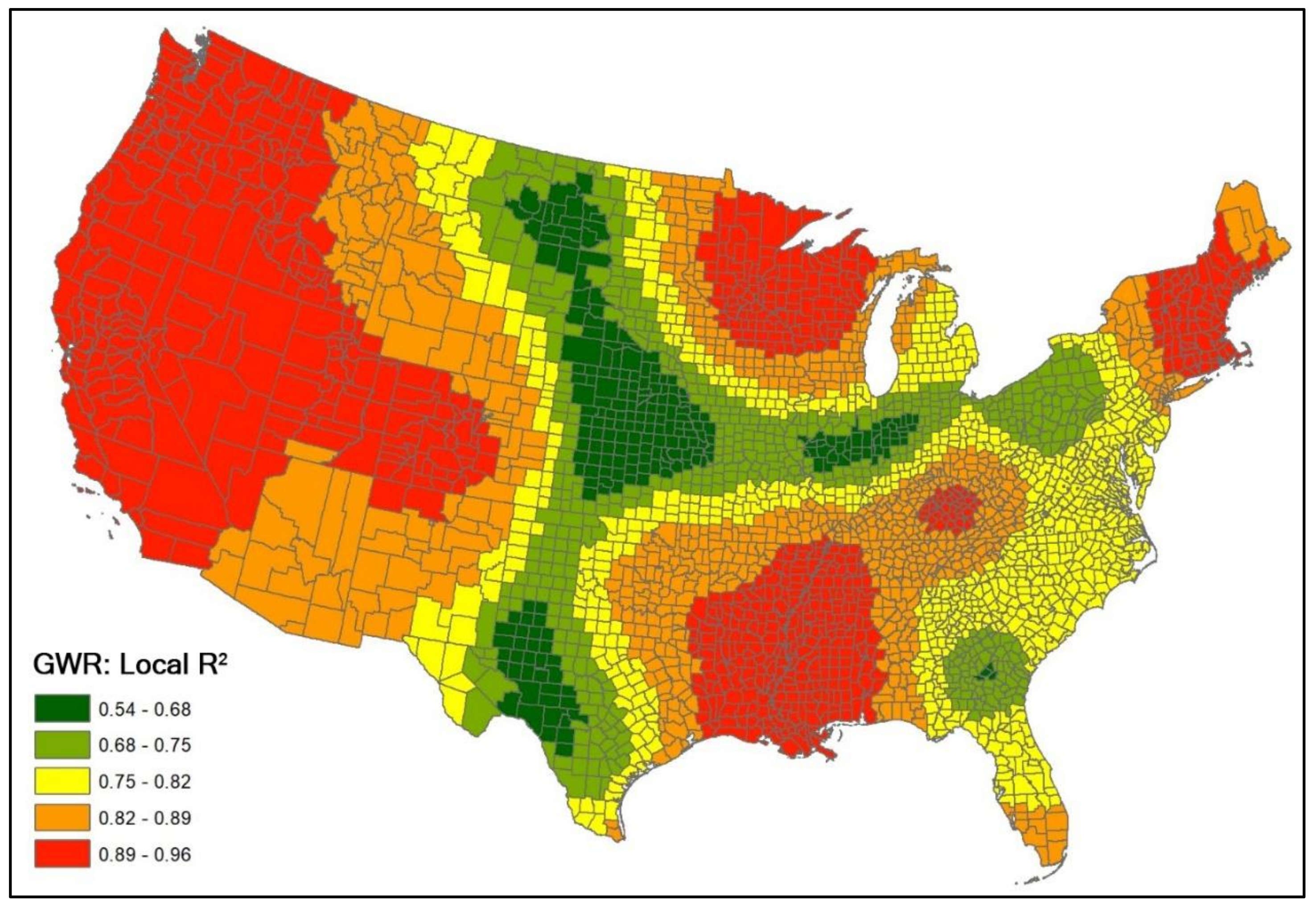
Figure 3.
Residuals of LTPI at the county level for SLM.
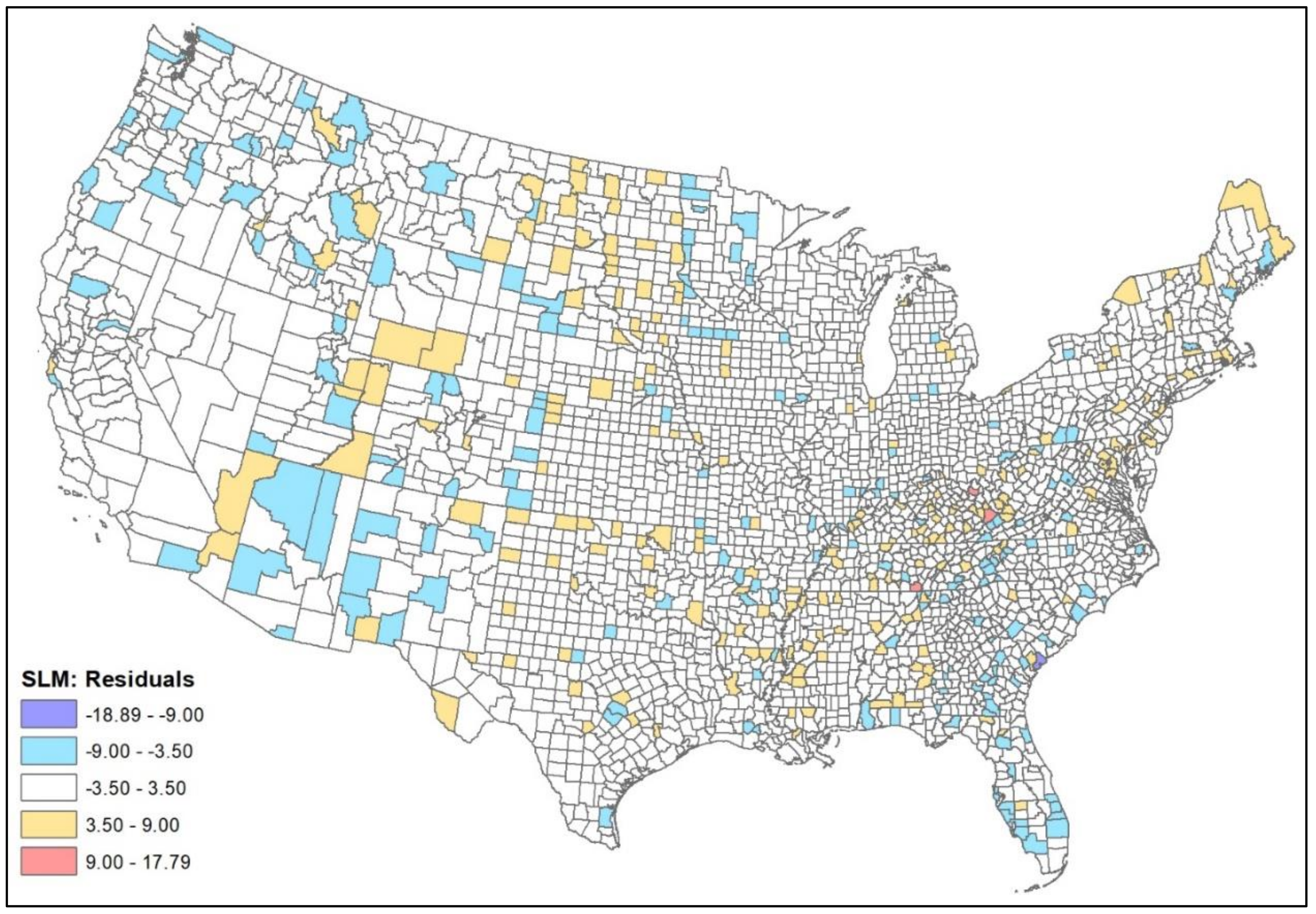
Figure 4.
Residuals of LTPI at the county level for GWR.

Figure 5.
GWR local coefficient between LTPI prevalence and tree canopy coverage at the county level.
Figure 5.
GWR local coefficient between LTPI prevalence and tree canopy coverage at the county level.

Figure 6.
GWR t-value of tree canopy coverage at the county level.

Figure 7.
GWR local coefficient between LTPI prevalence and the percentage of residents who are Asian.
Figure 7.
GWR local coefficient between LTPI prevalence and the percentage of residents who are Asian.

Figure 8.
GWR t-value of the percentage of residents who are Asian.


Table 1.
List of factors regarding physical environment, demographic characteristic, and socioeconomic status.
Table 1.
List of factors regarding physical environment, demographic characteristic, and socioeconomic status.
| Variable | Description | Year | Source | |
|---|---|---|---|---|
| Physical Environment | ||||
| Average annual temperature | Annually average daily temperature | 2011 | US Department of Agriculture (Schlenker & Roberts, 2009) | |
| Average annual precipitation | Annually average daily precipitation | US Department of Agriculture (Schlenker & Roberts, 2009) | ||
| Tree canopy | Percentage of tree canopy coverage | US Forest Service | ||
| Land cover | Density of highly developed areas with high ratios of residential, business, commercial, and industrial areas | Multi-Resolution Land Characteristics (MRLC) Consortium | ||
| Walkability | Minor road density | Topologically Integrated Geographic Encoding and Referencing (TIGER) | ||
| Demographic Characteristics | ||||
| Age | Median age (years) | 2011 | American Community Survey (ACS) | |
| Sex | Percentage of residents who are female | |||
| Race | African American | Percentage of residents who are African American | ||
| Asian | Percentage of residents who are Asian | |||
| Hispanic and Latino | Percentage of residents who are Hispanic and Latino | |||
| Socioeconomic Status | ||||
| Income | Income per capita (inflation-adjusted dollars) | 2011 | American Community Survey (ACS) | |
| Employment | Unemployment rate | |||
| Occupation | Management, business, science, and arts | Percentage of residents whose occupation are management, business, science, and arts | ||
| Natural resources, construction, and maintenance | Percentage of residents whose occupation are natural resources, construction, and maintenance | |||
| Production, transportation, and material moving | Percentage of residents whose occupation are production, transportation, and material moving | |||
| Self-employed unpaid family workers | Percentage of residents who are self-employed unpaid family workers | |||
| Commuting mode—work at home | Percentage of residents who are work at home | |||
| Commuting mode—walking | Percentage of residents commuting to work by walking | |||
| House ownership | Percentage of housing units that are owner-occupied | |||
| Vehicle ownership | Percentage of families have no vehicles available | |||
Table 2.
Descriptive statistics of physical and social environmental factors.
| Variables | Minimum | Maximum | Mean | Standard Deviation |
|---|---|---|---|---|
| LTPI | 10 | 45 | 27.15 | 5.06 |
| Temperature (°C) | −0.09 | 24.78 | 12.78 | 4.77 |
| Precipitation (inch) | 0.00 | 8.80 | 2.90 | 1.28 |
| Tree canopy coverage (%) | 0.02 | 92.25 | 34.64 | 25.87 |
| Land cover (%) | 0.00 | 48.42 | 0.52 | 2.15 |
| Walkability (km/km2) | 0.09 | 16.71 | 2.30 | 1.61 |
| Commuting mode 1—walking (%) | 0.00 | 31.30 | 3.23 | 2.75 |
| Commuting mode 2—work at home (%) | 0.00 | 42.00 | 4.92 | 3.50 |
| Occupation 1—management, business, science, and arts (%) | 11.10 | 67.60 | 30.35 | 6.44 |
| Occupation 2—natural resources, construction, and maintenance (%) | 1.00 | 52.50 | 13.28 | 4.30 |
| Occupation 3—production, transportation, and material moving (%) | 1.10 | 36.70 | 15.85 | 5.79 |
| Self-employed unpaid family workers (%) | 0.00 | 11.00 | 0.31 | 0.49 |
| Unemployment rate (%) | 0.00 | 18.40 | 4.80 | 1.90 |
| Income ($) | 7887 | 61,290 | 23,044 | 5460 |
| House ownership (%) | 20.10 | 93.70 | 73.15 | 7.69 |
| Vehicle ownership (%) | 0.00 | 78.00 | 6.30 | 3.64 |
| Age (year) | 21.60 | 62.20 | 40.14 | 4.97 |
| Female (%) | 24.20 | 59.20 | 50.54 | 2.78 |
| Race 1—African American (%) | 0.00 | 95.70 | 1.59 | 6.39 |
| Race 2—Asian (%) | 0.00 | 34.00 | 1.00 | 2.13 |
| Race 3—Hispanic and Latino (%) | 0.00 | 98.00 | 8.09 | 13.10 |
Table 3.
Summary of OLS and spatial lag models with LTPI as a function of physical environmental factors, socioeconomic status, and demographic characteristics for all U.S. counties.
Table 3.
Summary of OLS and spatial lag models with LTPI as a function of physical environmental factors, socioeconomic status, and demographic characteristics for all U.S. counties.
| Variables | OLS (Adjusted R2 = 0.606; R2 = 0.608; AIC = 16,063; F-Statistic = 239.7 (df: 3088); p-Value: 0.000; Log Likelihood = −8009.86) | SLM (Nagelkerke Pseudo-R2: 0.744; LR Test: 1320.8; AIC = 14,745; Rho (Spatial Lag) = 0.607; p-Value = 0.000; Log Likelihood = −7349.456) | ||
|---|---|---|---|---|
| Coefficient (95% Confidence Interval) | p | Coefficient (95% Confidence Interval) | p | |
| Temperature (β1) | 0.45 (0.42, 0.48) | 0.000 ** | 0.15 (0.12, 0.18) | 0.000 ** |
| Precipitation (β2) | 0.76 (0.63, 0.89) | 0.000 ** | 0.26 (0.15, 0.36) | 0.000 ** |
| Tree canopy coverage (β3) | −0.03 (−0.03, −0.02) | 0.000 ** | −0.02 (−0.02, −0.01) | 0.000 ** |
| Land cover (β4) | 0.07 (−0.02, 0.16) | 0.128 | 0.10 (0.03, 0.17) | 0.005 * |
| Walkability(β5) | 0.02 (−0.13, 0.09) | 0.736 | 0.08 (0.0004, 0.17) | 0.049 |
| Unemployment rate (β6) | −0.37 (−0.45, −0.30) | 0.000 ** | −0.10 (−0.16, −0.04) | 0.000 ** |
| Commuting Mode 1 (β7) | −0.07 (−0.13, −0.02) | 0.013 | −0.05 (−0.09, −0.005) | 0.029 |
| Commuting Mode 2 (β8) | −0.08 (−0.13, −0.03) | 0.000 ** | −0.04 (−0.08, −0.01) | 0.011 |
| Occupation 1 (β9) | 0.09 (0.05, 0.13) | 0.000 ** | −0.006 (−0.02, 0.01) | 0.445 |
| Occupation 2 (β10) | 0.19 (0.15, 0.22) | 0.000 ** | 0.13 (0.11, 0.16) | 0.000 ** |
| Occupation 3 (β11) | 0.17 (0.14, 0.20) | 0.000 ** | 0.09 (0.06, 0.11) | 0.000 ** |
| Self–employed unpaid family workers (β12) | 0.41 (0.14, 0.67) | 0.002 * | 0.19 (−0.01, 0.39) | 0.057 |
| Income (β13) | −0.0004 (−0.0004, −0.0003) | 0.000 ** | −0.0002 (−0.0002, −0.0002) | 0.000 ** |
| House ownership (β14) | 0.02 (−0.007, 0.04) | 0.178 | 0.02 (0.003, 0.04) | 0.023 |
| Vehicle ownership (β15) | 0.14 (0.09, 0.19) | 0.000 ** | 0.07 (0.04, 0.11) | 0.000 ** |
| Age (β16) | 0.08 (0.05, 0.11) | 0.000 ** | 0.09 (0.07, 0.12) | 0.000 ** |
| Female (β17) | 0.11 (0.07, 0.16) | 0.000 ** | 0.07 (0.04, 0.11) | 0.000 ** |
| Race 1 (β18) | 0.08 (0.06, 0.10) | 0.000 ** | 0.06 (0.04, 0.07) | 0.000 ** |
| Race 2 (β19) | −0.12 (−0.20, −0.05) | 0.000 ** | 0.02 (−0.03, 0.06) | 0.456 |
| Race 3 (β20) | −0.09 (−0.10, −0.08) | 0.000 ** | −0.04 (−0.05, −0.03) | 0.000 ** |
* Coefficient significant at p < 0.01; ** Coefficient significant at p < 0.001. AIC: Akaike Information Criterion. LR test: Likelihood rate test. Sample size: n = 3109.
Table 4.
Summary of GWR model coefficient estimates with LTPI as a function of physical and social environmental factors for all U.S. counties.
Table 4.
Summary of GWR model coefficient estimates with LTPI as a function of physical and social environmental factors for all U.S. counties.
| Variables | GWR (Adjusted R2 = 0.814; R2 = 0.856; AIC = 13,415) | |||||||
|---|---|---|---|---|---|---|---|---|
| Positive Coefficient Estimates (%) | Significant Positive Coefficient Estimates (%) † | Negative Coefficient Estimates (%) | Significant Negative Coefficient Estimates (%) †† | Minimum Coefficient Estimate | Median Coefficient Estimate | Maximum Coefficient Estimate | Significant Coefficient Estimates (%) ††† | |
| β1 | 77 | 72 | 23 | 21 | −0.4624 | 0.2880 | 1.7652 | 60 |
| β2 | 68 | 33 | 32 | 15 | −4.6594 | 0.2492 | 3.7850 | 27 |
| β3 | 22 | 25 | 78 | 44 | −0.2460 | −0.0177 | 0.1481 | 40 |
| β4 | 69 | 26 | 31 | 25 | −1.2027 | −0.1327 | 2.7811 | 26 |
| β5 | 34 | 24 | 66 | 40 | −3.0601 | −0.2528 | 1.2487 | 35 |
| β6 | 40 | 31 | 60 | 40 | −1.1192 | −0.0882 | 0.6460 | 36 |
| β7 | 30 | 1 | 70 | 30 | −0.7806 | −0.0882 | 0.1943 | 21 |
| β8 | 23 | 10 | 77 | 39 | −0.6463 | −0.1092 | 0.1500 | 32 |
| β9 | 37 | 28 | 63 | 16 | −0.2925 | −0.0224 | 0.3016 | 20 |
| β10 | 82 | 42 | 18 | 8 | −0.2153 | 0.0938 | 0.4111 | 36 |
| β11 | 82 | 34 | 18 | 13 | −0.1519 | 0.0651 | 0.3195 | 30 |
| β12 | 57 | 13 | 43 | 2 | −3.2365 | 0.1035 | 2.9226 | 9 |
| β13 | 2 | 0 | 98 | 86 | −0.0006 | −0.0003 | 0.0001 | 84 |
| β14 | 34 | 16 | 66 | 35 | −0.2633 | −0.0314 | 0.2317 | 29 |
| β15 | 60 | 35 | 40 | 24 | −0.6135 | 0.0376 | 0.7855 | 31 |
| β16 | 81 | 61 | 19 | 21 | −0.3432 | 0.1209 | 0.3409 | 53 |
| β17 | 83 | 37 | 17 | 10 | −0.4881 | 0.0983 | 0.3467 | 32 |
| β18 | 80 | 67 | 20 | 11 | −1.2628 | 0.1312 | 1.1136 | 56 |
| β19 | 24 | 47 | 76 | 39 | −1.4387 | −0.2622 | 0.3968 | 41 |
| β20 | 16 | 0 | 84 | 55 | −0.3264 | −0.0617 | 0.1640 | 46 |
† Number of positive significant (|t-value| ≥ 2.00) coefficient estimates/Number of positive coefficient estimates. †† Number of negative significant (|t-value| ≥ 2.00) coefficient estimates/Number of negative coefficient estimates. ††† Percentage of significant (|t-value| ≥ 2.00) coefficient estimates. AIC: Akaike Information Criterion. Sample size n = 3109.
Table 5.
Summary of 4 selected coefficient estimates of GWR model for the 20 most populous US counties
Table 5.
Summary of 4 selected coefficient estimates of GWR model for the 20 most populous US counties
| County | State | β3 | 95 CI | β5 | 95 CI | β13 | 95 CI | β19 | 95 CI | Local R2 |
|---|---|---|---|---|---|---|---|---|---|---|
| Santa Clara | CA | 0.0027 | (−0.06, 0.06) | −0.3870 | (−1.00, 0.23) | −0.0002 * | (−0.00, −0.00) | 0.1741 * | (0.03, 0.32) | 0.955 |
| King | WA | −0.0210 | (−0.06, 0.02) | 0.4379 | (−0.51, 1.38) | −0.0005 * | (−0.00, −0.00) | 0.3608 * | (0.01, 0.71) | 0.946 |
| Los Angeles | CA | −0.0358 | (−0.07, −0.00) | −0.4353 * | (−0.84, −0.03) | −0.0003 * | (−0.00, −0.00) | 0.1165 * | (0.01, 0.22) | 0.919 |
| Orange | CA | −0.0382 * | (−0.06, −0.01) | −0.3063 | (−0.66, 0.05) | −0.0003 * | (−0.00, −0.00) | 0.0535 | (−0.04, 0.15) | 0.910 |
| San Bernardino | CA | −0.0464 * | (−0.07, −0.02) | −0.3292 | (−0.68, 0.02) | −0.0003 * | (−0.00, −0.00) | 0.0594 | (−0.04, 0.16) | 0.906 |
| Clark | NV | −0.0625 * | (−0.09, −0.03) | −0.3423 * | (−0.67, −0.01) | −0.0003 * | (−0.00, −0.00) | 0.0698 | (−0.03, 0.17) | 0.902 |
| San Diego | CA | −0.0372 * | (−0.05, −0.02) | −0.1495 | (−0.45, 0.15) | −0.0003 * | (−0.00, −0.00) | −0.0264 | (−0.11, 0.06) | 0.898 |
| Riverside | CA | −0.0403 * | (−0.06, −0.02) | −0.1768 | (−0.48, 0.13) | −0.0003 * | (−0.00, −0.00) | −0.0162 | (−0.10, 0.07) | 0.898 |
| Maricopa | AZ | −0.0407 * | (−0.06, −0.02) | 0.0292 | (−0.24, 0.30) | −0.0003 * | (−0.00, −0.00) | −0.1413 * | (−0.23, −0.05) | 0.874 |
| Harris | TX | −0.0048 | (−0.02, 0.02) | −0.3865 | (−1.11, 0.34) | −0.0002 * | (−0.00, −0.00) | −0.1942 | (−0.45, 0.06) | 0.857 |
| Queens | NY | −0.0230 | (−0.05, 0.01) | 0.2636 * | (0.03, 0.50) | −0.0002 * | (−0.00, −0.00) | 0.1138 | (−0.05, 0.27) | 0.856 |
| New York | NY | −0.0221 | (−0.05, 0.01) | 0.2583 * | (0.01, 0.50) | −0.0002 * | (−0.00, −0.00) | 0.1110 | (−0.05, 0.27) | 0.854 |
| Kings | NY | −0.0222 | (−0.05, 0.01) | 0.2565 * | (0.02, 0.49) | −0.0002 * | (−0.00, −0.00) | 0.1132 | (−0.05, 0.27) | 0.851 |
| Dallas | TX | −0.0057 | (−0.03, 0.02) | −0.4800 | (−1.31, 0.35) | −0.0002 * | (−0.00, −0.00) | −0.3829 * | (−0.70, −0.07) | 0.850 |
| Miami-Dade | FL | −0.0201 * | (−0.03, −0.01) | −0.5922 * | (−0.78, −0.40) | −0.0004 * | (−0.00, −0.00) | −0.2133 * | (−0.40, −0.03) | 0.840 |
| Broward | FL | −0.0213 * | (−0.03, −0.01) | −0.6060 * | (−0.83, −0.39) | −0.0004 * | (−0.00, −0.00) | −0.2160 * | (−0.42, −0.01) | 0.835 |
| Tarrant | TX | −0.0057 | (−0.03, 0.02) | −0.5548 | (−1.35, 0.24) | −0.0002 * | (−0.00, −0.00) | −0.3952 * | (−0.70, −0.09) | 0.834 |
| Cook | IL | −0.0327 * | (−0.06, −0.01) | 0.0424 | (−0.36, 0.44) | −0.0003 * | (−0.00, −0.00) | −0.2707 | (−0.61, 0.06) | 0.798 |
| Wayne | MI | −0.0021 | (−0.02, 0.02) | 0.0073 | (−0.34, 0.35) | −0.0004 * | (−0.00, −0.00) | −0.2406 | (−0.68, 0.20) | 0.751 |
| Bexar | TX | −0.0164 | (−0.05, 0.02) | −0.6656 | (−1.62, 0.29) | −0.0002 * | (−0.00, −0.00) | −0.2040 | (−0.45, 0.04) | 0.699 |
95 CI: 95% confidence interval. * Significant coefficient estimates (|t-value| ≥ 2.00).
Table 6.
Summary of percentages of positive and negative coefficient estimates of GWR model for the 20 most populous US counties.
Table 6.
Summary of percentages of positive and negative coefficient estimates of GWR model for the 20 most populous US counties.
| β1 | β2 | β3 | β4 | β5 | β6 | β7 | β8 | β9 | β10 | β11 | β12 | β13 | β14 | β15 | β16 | β17 | β18 | β19 | β20 | |
|---|---|---|---|---|---|---|---|---|---|---|---|---|---|---|---|---|---|---|---|---|
| Positive Coefficient Estimates (%) | 65 | 60 | 5 | 80 | 35 | 15 | 45 | 0 | 50 | 100 | 95 | 65 | 0 | 70 | 85 | 90 | 85 | 85 | 45 | 10 |
| Significant Positive Coefficient Estimates (%) † | 69 | 25 | 0 | 13 | 43 | 33 | 0 | 0 | 0 | 45 | 47 | 38 | 0 | 14 | 35 | 50 | 35 | 82 | 33 | 0 |
| Negative Coefficient Estimates (%) | 35 | 40 | 95 | 20 | 65 | 85 | 55 | 100 | 50 | 0 | 5 | 35 | 100 | 30 | 15 | 10 | 15 | 15 | 55 | 90 |
| Significant Negative Coefficient Estimates (%) †† | 14 | 0 | 47 | 0 | 31 | 41 | 0 | 70 | 0 | 0 | 0 | 0 | 100 | 0 | 0 | 100 | 0 | 0 | 45 | 72 |
| Significant Coefficient Estimates (%) ††† | 50 | 15 | 45 | 10 | 35 | 40 | 0 | 70 | 0 | 45 | 45 | 25 | 100 | 10 | 30 | 55 | 30 | 70 | 40 | 65 |
† Number of positive significant (|t-value| ≥ 2.00) coefficient estimates/Number of positive coefficient estimates. †† Number of negative significant (|t-value| ≥ 2.00) coefficient estimates/Number of negative coefficient estimates. ††† Percentage of significant (|t-value| ≥ 2.00) coefficient estimates.
© 2018 by the authors. Licensee MDPI, Basel, Switzerland. This article is an open access article distributed under the terms and conditions of the Creative Commons Attribution (CC BY) license (http://creativecommons.org/licenses/by/4.0/).
Share and Cite
MDPI and ACS Style
Wang, J.; Lee, K.; Kwan, M.-P. Environmental Influences on Leisure-Time Physical Inactivity in the U.S.: An Exploration of Spatial Non-Stationarity. ISPRS Int. J. Geo-Inf. 2018, 7, 143. https://doi.org/10.3390/ijgi7040143
AMA Style
Wang J, Lee K, Kwan M-P. Environmental Influences on Leisure-Time Physical Inactivity in the U.S.: An Exploration of Spatial Non-Stationarity. ISPRS International Journal of Geo-Information. 2018; 7(4):143. https://doi.org/10.3390/ijgi7040143
Chicago/Turabian StyleWang, Jue, Kangjae Lee, and Mei-Po Kwan. 2018. "Environmental Influences on Leisure-Time Physical Inactivity in the U.S.: An Exploration of Spatial Non-Stationarity" ISPRS International Journal of Geo-Information 7, no. 4: 143. https://doi.org/10.3390/ijgi7040143
Note that from the first issue of 2016, this journal uses article numbers instead of page numbers. See further details here.