Assessment of Accuracy in the Identification of Rock Formations from Aerial and Terrestrial Laser-Scanning Data

Abstract

Rock formations are among the most spectacular landscape features both for experts and the public. However, information about these objects is often stored inaccurately in existing spatial databases, their corresponding elevations are missing, or the entire rock object is completely absent. Cartographic depiction is also reduced to a point of areal symbology of a largely generalized character. This paper discusses options in identifying and analyzing rock formations from two digital terrain models (DTMs), DMR 5G and DMR 5G+, and irregularly spaced points of airborne laser-scanning (ALS) data with different point densities. A semi-automatic method allowing rock formations to be identified from DTMs is introduced at the beginning of the paper. A method to evaluate elevation models (volume differences) is subsequently applied and a 3D model of a selected rock object is created from terrestrial laser-scanning data. Finally, positional and volumetric comparisons of that 3D object are performed in 2D, 2.5D, and 3D. The results of the pilot study confirmed that the digital terrain models studied are a reliable source in identifying and updating rock formations using the semi-automatic method introduced. The results show that DMR 5G model quality decreases with increasing fragmentation and relative rock formation height, while the proportion of gross errors increases. The complementary DMR 5G+ is better in terms of location and altitude.

1. Introduction

The growing demand today for detailed topographic data in 3D reflects the development of technological solutions, acquisition, and data-processing options. Accurate altitude data are crucial for modeling events, such as flooding, power transmission within a city’s thermal island, or radio-signal propagation. In addition to the private sector, which maps smaller areas and adapts to market behavior, national mapping agencies create 3D topographic databases for the needs of strategic urban planning and more accurate derivation of cartographic products [1].

Laser-scanning data for digital surface models (DSM) and digital terrain models (DTM) have been used in several European countries such as the Netherlands, Poland, and Finland, or used as a data acquisition source in Catalonia, Bavaria and Switzerland [1,2,3,4,5].

In the Czech Republic, airborne laser-scanning (ALS) data processing was completed in 2016 under a project approved in 2008 to create new altimetry. Scanning was mostly performed in blocks of 10 × 30 km and counted with a 50% overlap of neighboring strips. Scanner and flight height settings were based on the scanning period. Scanning was carried out from a height of 1200 m above the terrain with a pulse transmission frequency of 80 kHz at the time of vegetation growth; at other times, the mean flight height was 1400 m and the scanning frequency increased to 120 kHz. Due to high vertical differences, flight height was reduced to just 800 m over mountains. As a result of the transverse overlap of belts, a point cloud density of 1.6 points/m² was achieved [6]. This project depended on the creation of three derivative digital model products: DMR 4G, DMR 5G, and DMP 1G. The fourth generation Digital Terrain Model (DMR 4G) of the Czech Republic is a model with a regular point grid, resolution of 5 × 5 m, and vertical root mean square error (RMSE) of 0.3 m in exposed terrain in areas covered with vegetation 1 m high and designed primarily for creating true orthophotos or less-complicated analyses. The 1st generation Digital Surface Model (DMP 1G) of the Czech Republic is created with irregularly spaced points. This model is the first product of its kind in the Czech Republic and designed for analyzing the heights of objects on the Earth’s surface. The vertical RMSE is 0.4 m in open and well-defined areas and 0.7 m in locations frequently covered with vegetation. The 5th generation Digital Terrain Model (DMR 5G) of the Czech Republic is a network of irregularly spaced points with vertical RMSE accuracy of 0.18 m in exposed terrain and 0.3 m at sites covered with vegetation. It is currently the most accurate terrain model of the Czech Republic and may be used in various physical geographical analyses of areas during initial stages of urban planning or other land modifications [7]. All data models are designed as 2.5D, so the models are unable to find more than one altitude for a location. This is particularly clear on the walls of houses in DMP 1G, where the bottom edges of walls protrude about 10 cm outside the house. DMR 5G+ is a pre-finalized product with several filtered points that are not normally available on land survey office websites, and therefore similar statistics or RMSE in an exposed or covered area are not available. This model, however, has a slightly higher point density (0.165 points/m² vs. 0.125 points/m²) than DMR 5G and leaves more points on a terrain skeleton.

The model’s accuracy assessment was carried out on a wide scale on fairly ideal surface terrain types and points of the fundamental horizontal geodetic control or additionally created geodetic control points. This type of evaluation characterizes the resulting products mainly from the point of view of internal variability rather than absolute height error which, as described in the modeling methodology [8], can achieve higher vertical differences. Although RMSE reliability is high and calculated as a triple of the standard deviation between geodetic control points and a model derived from airborne laser-scanning data, this evaluation is subject to a systematic error generated by the locations and characteristics of the test points. The laser-scanning method for collecting topographic data has some limitations regarding measurement accuracy and, therefore, the role of errors stems from the topographic nature of an area, which may be regionally completely different from the overall assessment of the altimetry model [9,10]. It is assumed that areas with higher vertical differences in territories with no ideal surface type will record higher elevation differences. Therefore, sites with rock formations characterized by higher vertical differences and more different shapes were selected as relief test types.

The presented study discusses the potential use of the DMR 5G model in identifying and assessing the accuracy of capturing rock formations from airborne laser-scanning data. Rock outcrops as edges of landslides were looked for and validated with the ALS DTM in Poland. Altitude, slope, slope orientation, and relief energy were selected as the main search parameters in the DTM [11]. Automatic facet detection on rocky surfaces was investigated in [12]. During identification, the varying density of the point cloud and its influence on the success of classification was tested. The theoretical approach to defining rock formations and the quality of the DTM model has been dealt with in [10]. The main aims of this paper are to:

-

identify localities with rock formations from DMR 5G+;

-

assess the accuracy of DMR 5G and DMR 5G+ at these sites;

-

validate this assessment by creating a true 3D model of a rock formation.

After the introduction describing state-of-the-art DTM development in the Czech Republic, the paper is structured as follows: Section 2 describes potential errors encountered in laser scanning as well as the methods for evaluating height models by calculating volume difference, on which rock formation evaluation is based. Also, a semi-automatic method for detecting rock formations is specified together with an assessment of elevations in a 3D control model of a selected rock formation that is created from terrestrial laser-scanning data. A pilot study of Žďárské vrchy is described in detail in the following section and its results are compared with existing studies. The final discussion summarizes the main achievements and proposes possible follow-ups.

2. Theoretical and Methodological Background of Laser-Scanning Spatial Data

During its brief history and from its first introduction in the 1960s, the development and use of laser for collecting topographic data has made major steps forward. Today, laser scanners have a wide range of usable wavelengths of varying power and are either used as static (total station) or mobile (airborne or terrestrial systems) devices [13]. The development of measuring methods follows a similar trajectory. The basic principle of measuring objects is to record the time between the emission and capture of a reflected laser beam. This time-of-flight can then be recalculated to the metric distance p_i, thereby obtaining the relative distance of the object from the laser scanner. It is also necessary to record the location of x_lu, y_lu, (GPS—global positioning system), scanner orientation x_b, y_b, (IMU—inertial measurement unit) and the direction of the laser beam x_lb, y_lb, z_lb (laser unit) at the time of emission. Based on the known coordinates of the scanner, its orientation, and calculated object distance, each point can then be precisely located with absolute coordinates X_m, Y_m, Z_m relative to the origin of the coordinate system [14]. Other traditional methods of measurement include continuous mode, full-waveform mode [15], or multispectral mode similar to multispectral imaging [16]. Perhaps the most up-to-date, efficient, and accurate method currently is the so-called single photon lidar. This method has lower energy demands and allows faster data collection compared to conventional solutions [17]. Regarding mapping with laser scanning, we can take into account three error groups that may affect the primary point cloud quality:

• Errors caused by the technologies used.
• Errors caused by atmospheric conditions.
• Errors caused by reflections from objects.

Errors caused by technologies stem from internal scanning settings and include errors in clocks, detectors, scanning devices, navigational and geodetic devices, and communications between devices [13]. They also include errors in transmitted beam parameters and distances of objects measured by laser scanners. A transmitted laser beam passing through an atmospheric layer changes its original properties. Errors caused by atmospheric conditions include atmospheric refraction, extinction, and diffraction divergence of the laser beam, whose size mainly depends on temperature, pressure, humidity and purity of the atmosphere, as well as beam wavelength and overall length and emission direction. Errors caused by reflections from objects are affected by the reflectivity of objects, surface roughness, angle of beam incidence, and multipath. A more detailed description of errors and the functioning of each system component can be found in textbooks, such as [13] or [14]. It was not possible to measure all these variables throughout the project, therefore this paper only evaluates the cumulative error of the data. It is always necessary to compare a device with alternative methods, such as stereophotogrammetry or tachymetry, since parameters such as speed and data-acquisition accuracy are relative in this respect.

Creating Digital Elevation Models and Evaluating Accuracy

Since modern laser scanners operate at a high frequency [18], large point cloud datasets are created. In addition to the absolute number of points, the point density usually planned according to the purpose for capturing this data is important. These point clouds are computationally challenging in post-processing, so common point cloud filtering (e.g., removing error reflections, removing points on objects not part of the mapping project, removing redundant points on overlapping scanning strips) is necessary. The result is sparse point clouds, most often irregularly spaced points, usable for creating digital-elevation models. Point cloud processing to reconstruct and render detailed 3D model objects and storage structures is described, for example, by [19].

Digital elevation models of the Earth’s surface from laser scanners are most commonly stored and distributed as point clouds [1]. Based on these data, continuous grid-based and triangle-based models are reconstructed. While grid-based models are the result of point cloud interpolation, triangle-based models connect points into triangular structures where, when using a Delaunay triangulation, the same model is always obtained. In terms of interpolation, this may not always be achieved if geostatistical methods of interpolation are used for working with an element of randomness (e.g., kriging). The spatial resolution of a single pixel also plays a significant role. Although this value can be derived from the average distance of the nearest neighboring points, it fails to reflect frequent non-homogeneity of the point cloud density (resulting from the scanning principle or processing techniques) and is thus distorted [20,21]. This fact influences the evaluation of a model’s accuracy, where different results moving in a different range of values are always obtained. Additionally, triangle-based models capture important natural breaklines in the landscape and thus do not smooth the resulting model as much as grid-based models.

Several approaches can be employed to assess accuracy, and each has its advantages and disadvantages. We can mention methods to evaluate the network of irregular triangles, raster grid of a digital model, or volume difference, or assign information from the nearest neighboring points. Heights can be compared across categories of surface types, in different geomorphological conditions, or with different stages of product processing [20]. In Earth sciences, scenes are modeled more planarly than as fully 3D scenes. Therefore, we can compare these 2.5D models stored horizontally with the methods listed above. The evaluation of height models derived from airborne laser scanning in the Czech Republic was performed with [22] or [23]. Apparently, the most commonly used evaluation of these data using volume difference can be found in the works of [9,23,24,25]. The method is based on interlacing the test and reference model in the form of a triangle-based model across the test area. The quality and error parameters of the tested elevation model are derived from the resulting differential model. Regarding the data obtained by airborne laser scanning, more errors can be expected in places with higher vertical differences or areas with inappropriate material or surface type for this specific data-collection method.

Obviously, some of the most probable locations in the open landscape prone to error are rock formations partially hidden by forest. Their shape and height may be affected by incorrect classification of the original points or by some of the filtration methods. These sites are frequently popular tourist sites or landmarks and are often used for modeling visibility characteristics. Therefore, it is necessary to identify these locations in point clouds correctly and maintain their height and position as accurately as possible. The method for determining the position of these objects and the possibilities for assessing the quality of the entry for elevation models is discussed in the following chapter.

3. Methods

A digital terrain model is the final result of processing all the last reflections of emitted beams. When working with raw data, rock formations and unshaded terrain can, in most cases, be distinguished from the first reflections of the surrounding vegetation based on the amount and form of reflected energy, since more energy is reflected from a solid surface than the partially penetrable layer of a tree floor [13]. Regarding terrain under vegetation (or similar, partially penetrable objects), the last point of multiple reflection of the emitted beam is taken into account. In the case of a processed point cloud, all this information may be missing, and only the geometrical information in the form of X, Y, Z coordinates is available. To identify the rock formations, it is necessary to consider the geometric assumptions of the formations and possible locations of their occurrence. This processing system is very similar to the basic assumptions of raw data filtering [26].

A rock formation is most commonly characterized by a high inclination of slope and well-identified edges (it can also be an isolated structure), a compact object in terms of space (it is distinguishable from isolated boulders), and with vegetation rarely higher than small shrubs (except wood species, e.g., pine trees).

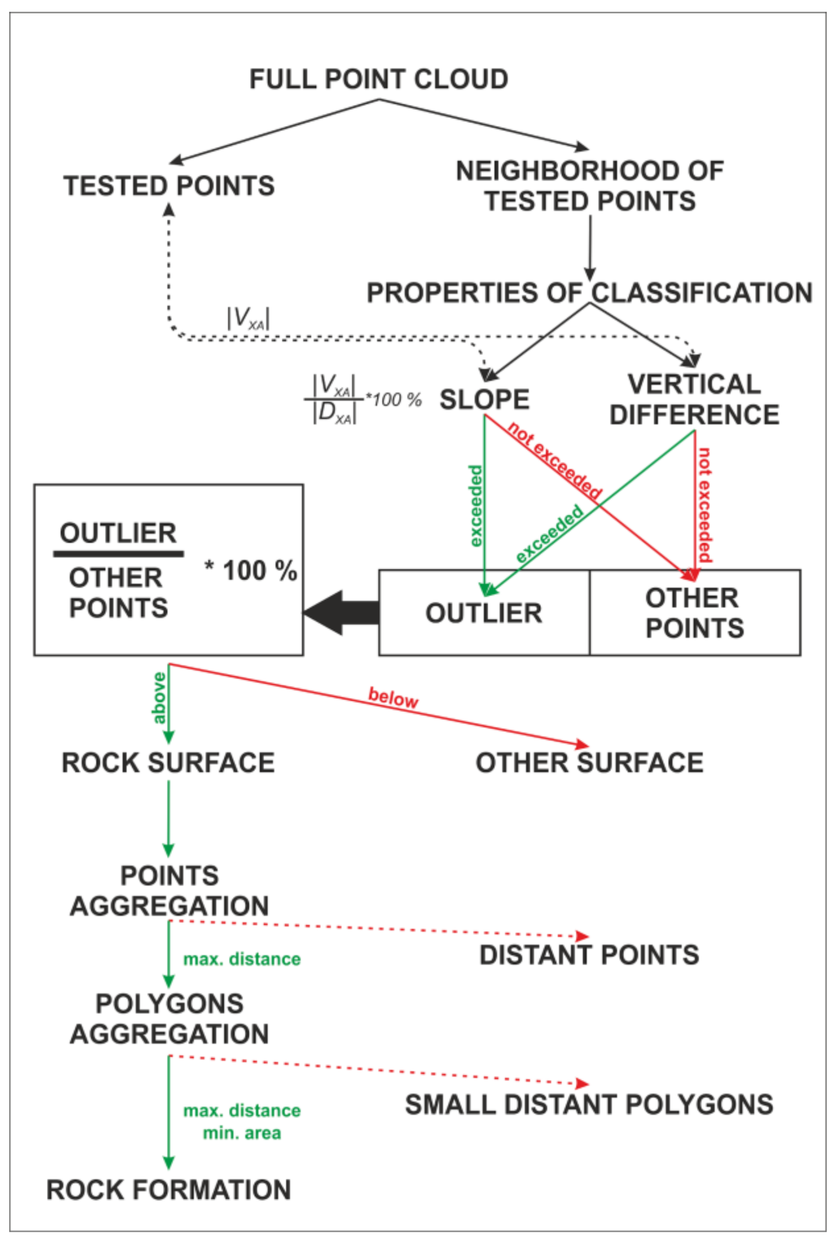
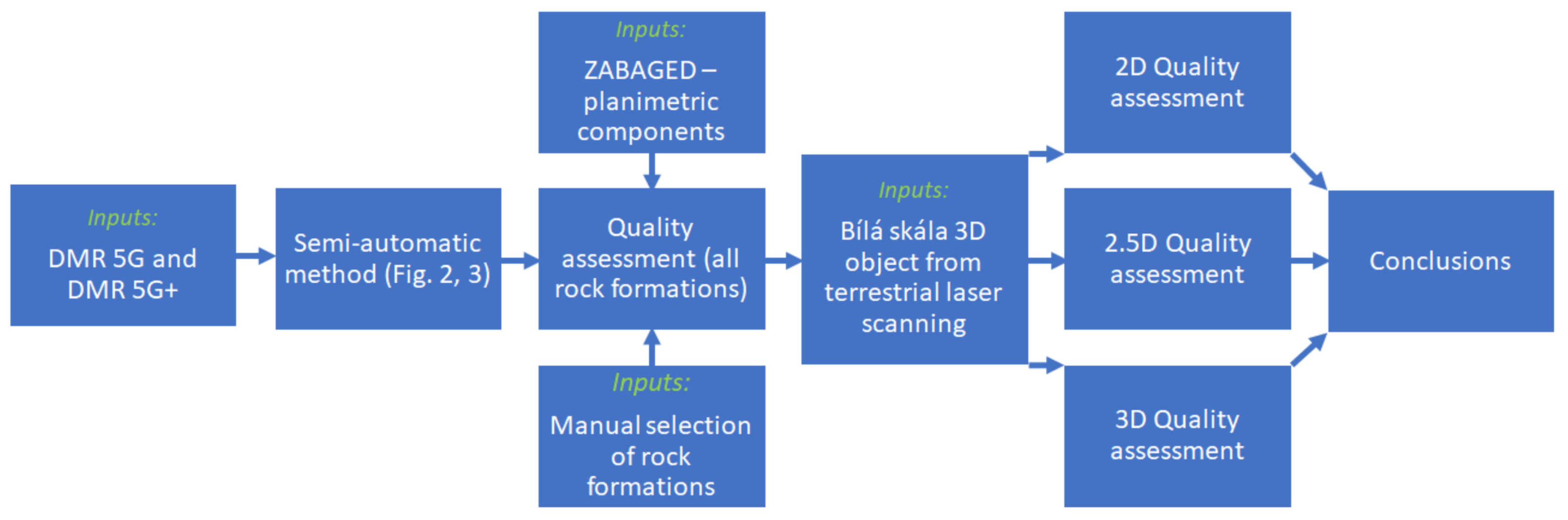
Figure 1 shows the whole process of identifying points located on the surface of these rock formations in the DTM point cloud, the spatial definition of individual rock formations, the assessment of their accuracy based on the existing topographic database, and detailed 3D modelling from terrestrial scanning.

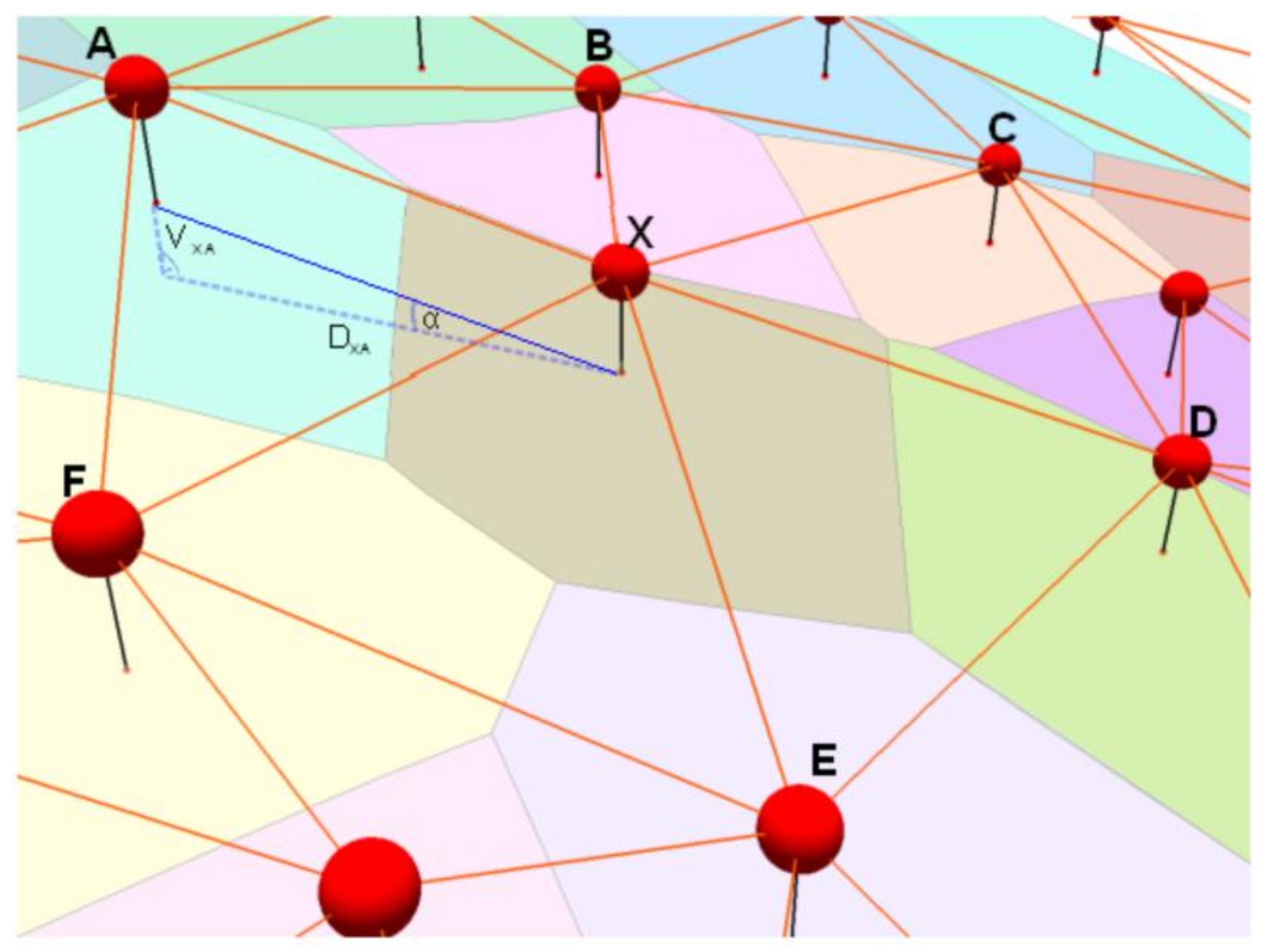
The initial identification of points lying on a rock surface can be performed with a semi-automatic method based on evaluating the nearest neighbors around individual points in 2.5D terrain. Surface discontinuities are defined by the vertical difference of neighboring points, the slope size, and the number of outlying points. The neighborhood of each point is defined by a Delaunay triangulation and Thiessen polygons, each point in the polygon having an irregularly shaped area. Its shape and size depend on the number and spacing of surrounding neighbors. The maximum vertical difference between the tested point is determined for each neighboring point, and if this difference is exceeded, the neighboring point is marked as an outlier. It is thus possible to search for points that vary considerably from their surroundings and show certain slopes in the terrain. Furthermore, the maximum allowed vertical difference threshold is defined in relation to the horizontal length at which this elevation changes. This limit can be expressed as a percentage where 100% indicates a slope of 45°, so the two edges of this triangle are the same length. Extreme values in this situation are 0% (no vertical difference) and ∞ % (means the vertical wall). Once this limit is exceeded, the neighboring point is again marked as an outlier. For both search settings, it is also necessary to determine the percentage of points near the tested point where the maximum admissible value of the aforementioned characteristics must be exceeded. For example, setting 70% means that to mark the tested point as an outlier at least 70% of the neighboring points must exceed the maximum admissible value of the given characteristics. The principle of identifying outlying points is shown in Figure 2.

The tested point X is vertically and horizontally distant from point A by V_XA and D_XA, which defines the spatial angle α, which is used to evaluate the maximum admissible percentage deviation of points. In this way, the other surrounding points B to F are tested and, based on their results and the set point of the vertical difference of surrounding points, the tested point X is marked as an outlier or not. When combining and setting these limits correctly, the points are selected so that they mostly define the areas of vertical obstacles in the area, in this case rock formations.

It is obvious that some rock formations may have round tops that are not selected in this way. This method must be completed with the process of aggregating close points according to their location in 2D into individual polygons. A major influence on polygon formation by aggregation from point data is applied by setting the maximum mutual distance for point attachment to other clustering points. If the selected distance is too small, a large number of separated polygons would be created, dividing real rock formations into several parts. By contrast, when determining a long distance, clusters of remote points would be formed to create an unreal rock massif. This parameter is mutable and depends primarily on the average distance between the nearest neighbors of the point cloud as well as knowledge of the environment in which the rock formations are located. The whole process of searching for rock formations was processed in ArcGIS 10.2.2 and is shown in Figure 3.

Determination of the lower and upper edges of airborne laser scanning was solved by [27]. The authors defined the basic prerequisite for calculating the positive and negative curvature of the terrain (grid-based), which gives the location of the edges. Subsequently, these edges are vectorized and the height is transferred from the underlying DTM. Knowledge of the environment can also be understood as the availability of a support data source for land cover and land use. As a result, formations can only be looked for in areas where they are expected to occur.

Modeling and assessing the accuracy of rock formations is now more or less reduced to monitoring the stability of slopes and rock blocks and performed in the case of laser scanning from terrestrial static stations [28,29]. Regarding the assessment of accuracy of rock formations from airborne laser scanning, it is obvious that the point cloud density on these objects is several times lower and is influenced by a different scanning direction. However, spatial deviations in the X and Y axes can be evaluated based on determining the lower and upper edges. The method called multiscale model-to-model cloud comparison (M3C2) can even calculate the X, Y and Z axes on individual rock walls using the local terrain model [30]. This method is not only limited to the nearest neighbor, but to the entire user-defined neighborhood of the point. Its main advantage is usability for different scales and the elimination of the problem of varying point cloud density. The resulting information gives an idea of the reliability of the digital terrain model in extreme locations and can be used to compare and potentially update topographic data. In the next chapter, DMR 5G+ is used for searching rock formations, and the evaluation methods presented in this section are used on a selected area. Another part of the evaluation is carried out on the selected rock formation Bílá skála, which was modeled as a reference from terrestrial scanning data.

4. Empirical Elaboration of the Field Campaign

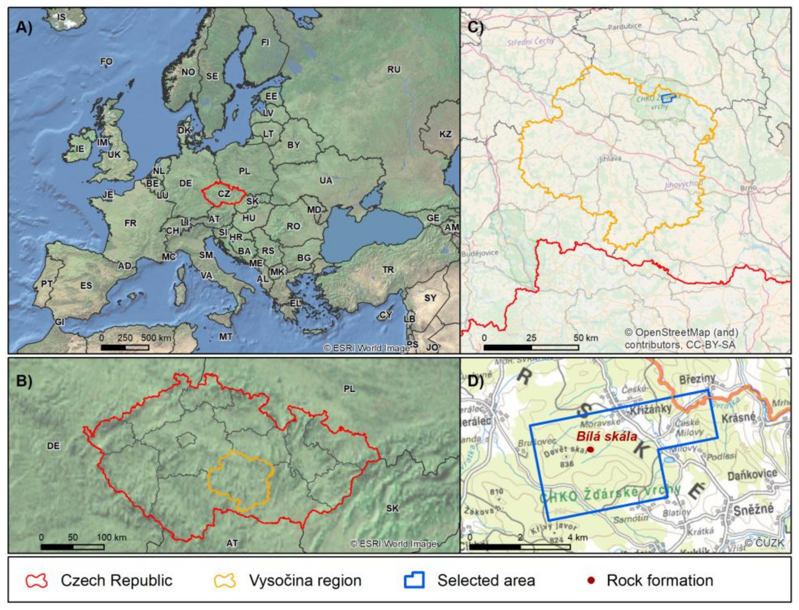
An area of approximately 25 km² in the Protected Landscape Area of Žd’árské vrchy (Figure 4) was selected as a study site. Folding processes here formed ridges predominantly in a south-east–north-west direction, where more resistant migmatites and metagranites formed relatively broad ridges originally separated by widely opened valleys that gradually narrowed and deepened. In the areas at the peaks of the ridges, it is often possible to encounter rock formations tens of meters high. The rocks have vertical walls facing most cardinal directions and slopes with slight gradients formed by boulders and streams created by polyhedral rocks. Most of the area is covered with coniferous forests or permanent grass fields. Small municipalities are in the northern and north-eastern part of the area.

4.1. Evaluation of DMR 5G Quality at the Selected Location in Žd’árské Vrchy

Data from DMR 5G as well as DMR 5G+ were used from the selected area. In addition, the digital database ZABAGED^® (Fundamental Base of Geographic Data of the Czech Republic), which is the main source for creating topographical maps in the Czech Republic in scales 1:10,000 to 1:100,000, was used for object type selection. ZABAGED^® has planimetric components containing 117 types of objects with a predominant postitional RMSE of up to 5 m. ZABAGED^® has a wide range of data sources, which are described in the ZABAGED^® Object Catalog [31].

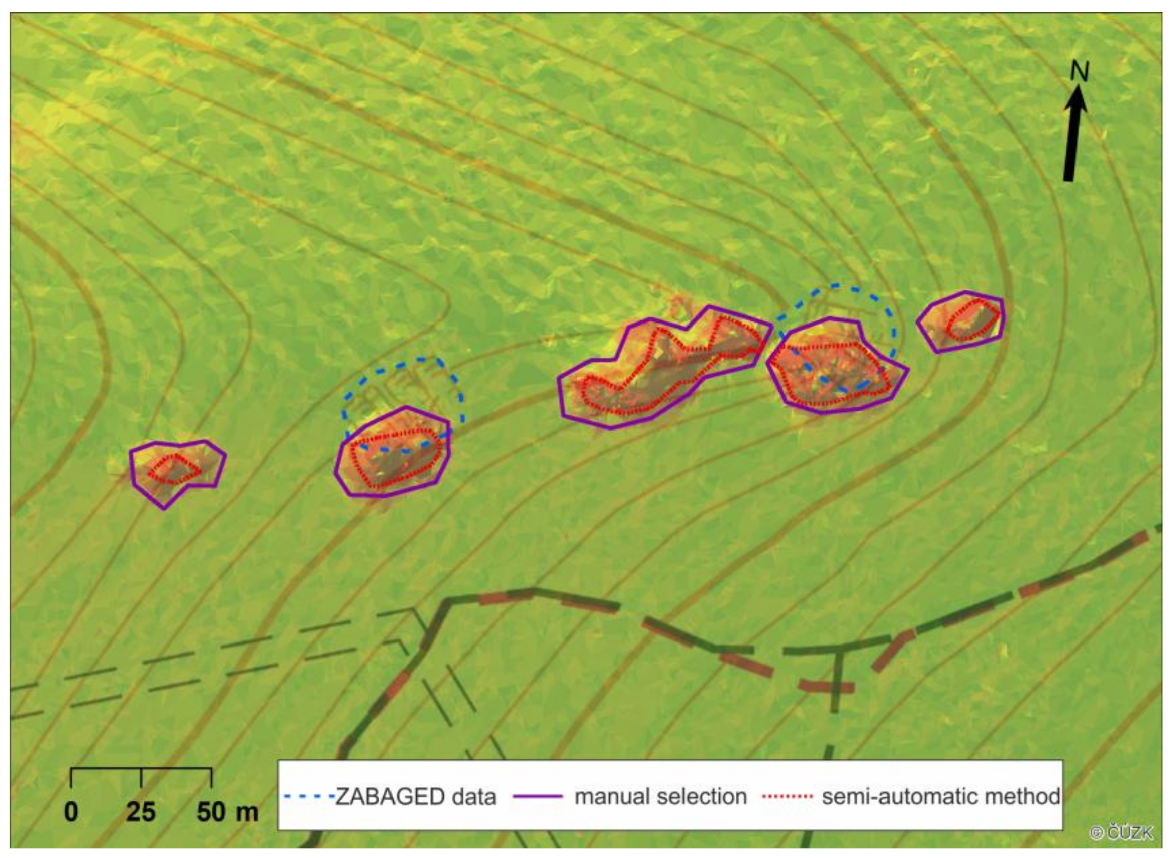
The first part of the assessment is an identification of rock formations from DMR 5G+ using the semi-automatic method. Using ZABAGED^® planimetric components, it is possible to determine the land-cover types where these objects will not occur (built-up municipal areas, water areas, meadows) and where the probability of occurrence is highest (forested areas). Rock formations as a type of object are part of ZABAGED^®, but the accuracy of markings is rather indicative of the initial mapping scale of 1:10,000. Therefore, this information can only be used as default information for determining the type of surfaces where these objects occur. For their true identification, DMR 5G+ was used and semi-automatic methods were applied. As mentioned in the Introduction, DMR 5G+ has a higher point density that makes it more suitable for searching for vertical barriers. An average horizontal distance of 1.3 m between points was found in this study area. This value can also be used to set the semi-automatic method parameters.

In general, higher vertical differences mean lower horizontal distances of points than those measured in planar locations (with respect to 50% lateral overlap of the strips). To exclude points that are too close (e.g., as a result of joining neighboring strips), a minimum vertical difference is required. Here, we can draw on the average horizontal distance of points and use this value as a vertical boundary. Based on this process, the inclination of rock formation slopes can be determined to an angle of 45°. Most likely, the walls will have a steeper gradient, although specifying this angle will exclude neighbors that are caused by the non-homogeneity of the point cloud and that meet the height limit over a long distance. Lastly, we need to specify a value for evaluating the outlying distance of a point from its neighborhood. From a bird’s-eye view, rock formations are generally convex, so the remote point must conform to that condition. Therefore, taking into account the expected vertical differences, a 30% boundary was set, indicating that the test point would be evaluated as an outlier if at least 30% of the neighboring points exceeded the angular and elevational limit. By applying these settings, clusters of points are searched for in the rock formations. For their delineation, points need to be aggregated into polygons and exclude those that are not rock formations. This can be done by specifying the minimum size of the polygon surface.

Since the contour model of ZABAGED^® does not include surface modeling of rock objects, a layer based on manual polygon definition and shaded slope relief of DMR 5G+ is created for positional comparison. Another possible alternative would include combining different directions and terrain elevations and creating multi-component shading reliefs. The method of volume difference and identifying gross errors presented in the works of [9,24,32] and [23] can also be used for height accuracy. However, in contrast to the ZABAGED^® altimetry reference model, DMR 5G + and DMR 5G are tested. Regarding the calculation of volumes, an approach is used where both models are in the triangle-based structure, and by subtraction create bodies which can be subsequently calculated for their volume. An essential part of the process is to determine absolute error as m_h, systematic errors s_h, and the proportion of gross errors [23]. Equations for calculating variables are as follows:

$$s_h=\frac{\Sigma V}{S}$$

(1)

$$m_h=1.25a_h$$

(2)

$$ah=\frac{\Sigma \left|V\right|}{S}$$

(3)

$$H_{ch}=\frac{S_{hch}}{S}$$

(4)

where s_h is calculated as a sum of all the positive and negative volumes divided by the total area under these volumes, a_h similarly adds positives and negative volumes but has absolute values, and H_ch calculates gross error as a triple of the standard deviation S_hch between elevations of both models which is divided by the total tested area.

4.2. Evaluation of DMR 5G Quality on the Selected Rock Formation

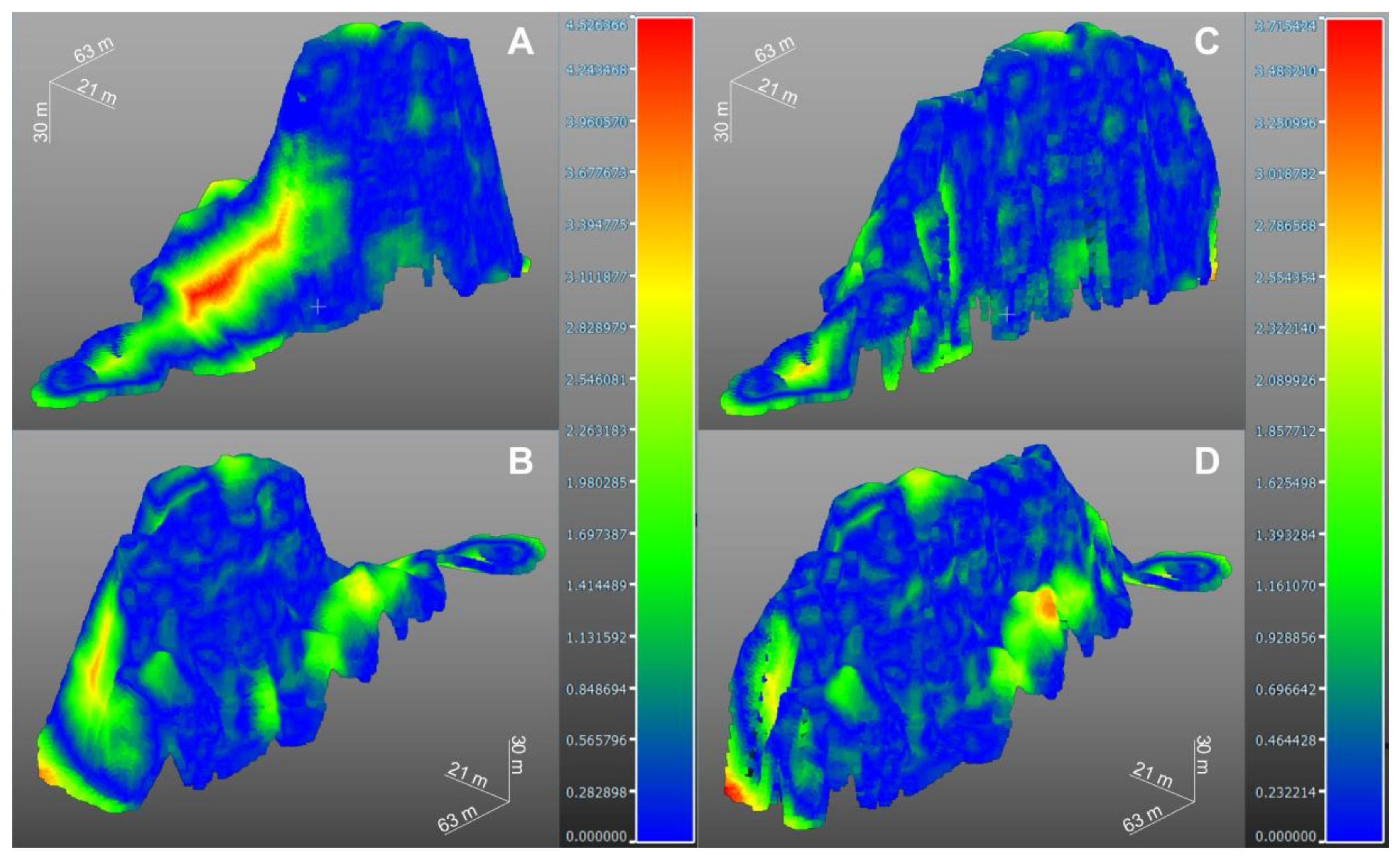
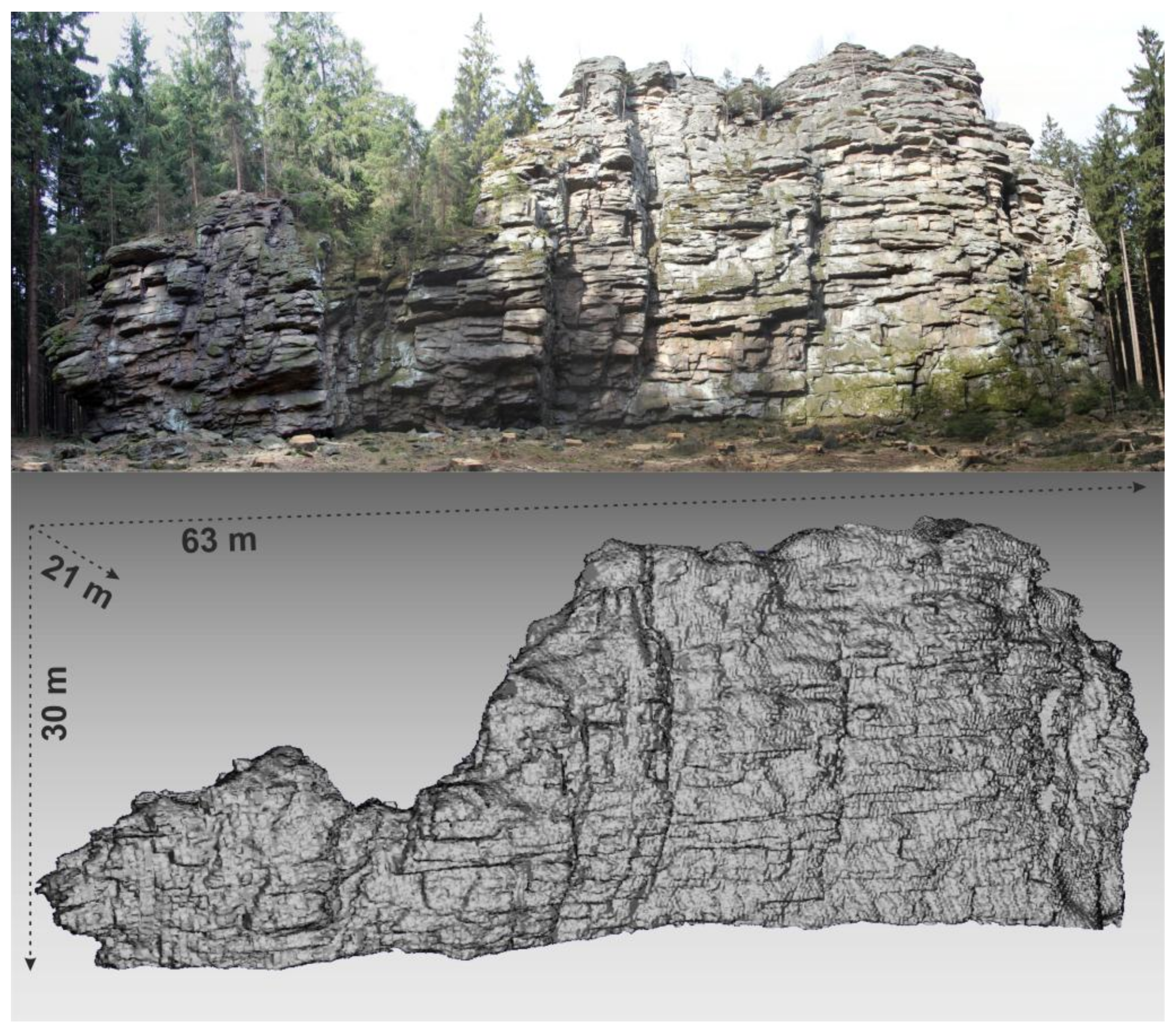
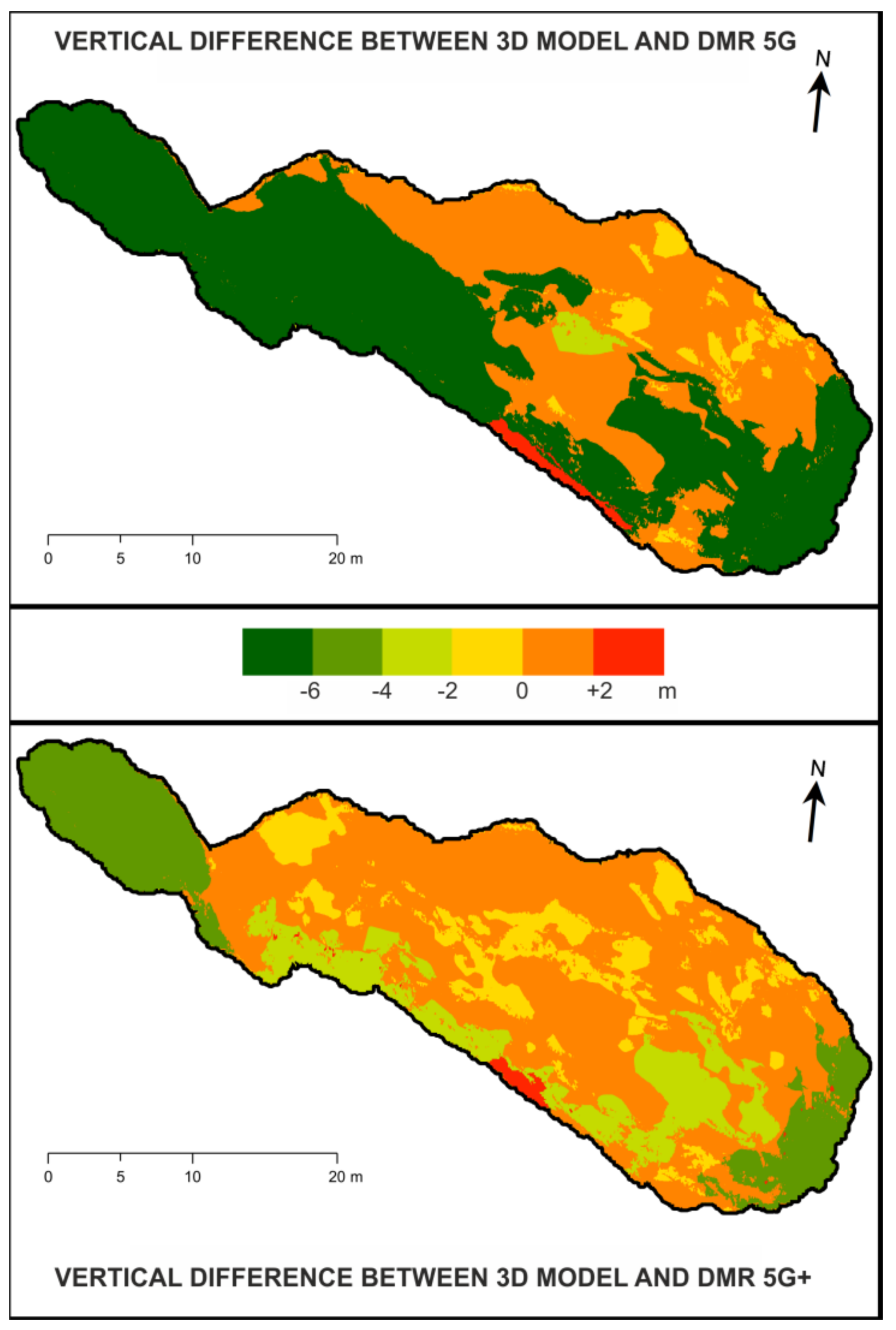
Due to the pilot study indicating that the DMR 5G+ model does not capture rock formations precisely, mapping was performed using a terrestrial laser scanner at the selected rock formation called Bílá Skála to evaluate absolute accuracy and assess the impact on its cartographic representation. This rock object is almost 30 m high and about 63 m long. Its broadest width is 21 m [33].

The FARO Focus3D X 130 laser scanner was used for terrestrial scanning. This device performs near-infrared laser scanning at a wavelength of 905 nm. The emitted beam has a divergence of 0.19 mrad and power of 20 mW. The guaranteed maximum measurement error is 2 mm at 25 m for materials with a reflectivity of 10%. At the time of scanning (autumn 2014), the closest neighborhood of Bílá skála was wooded, making it impossible to scan from minimum positions. Therefore, scanning from nine positions with an average horizontal length from the rock block of 15 m was chosen. The merging of individual scans was based on finding regularly spaced identical points representing white and highly reflective reference spheres with a total RMSE of up to 2 mm. The position of the scanner stations was determined by the Real Time Kinematic (RTK) system. Corrections were used in the navigational signal transmitted by the mobile network so that precision could be characterized by total RMSE of 1 cm. After filtering the surrounding vegetation and other points outside the rock object (both in Autodesk Recap), a total of 2,000,000 points remained. This point cloud combined most of the errors that can be encountered during terrestrial scanning—point density variability, holes caused by shadows behind objects and erroneous measurements. After processing the point cloud into a closed 3D model, 850,000 points remained in the object (in Geomagic Wrap 2014), that is, 1085 p/m². This model was tested with the M3C2 method (see Section 5.2) and can be characterized by total RMSE of 11 cm. The resultant model and its real form can be seen in Figure 5.

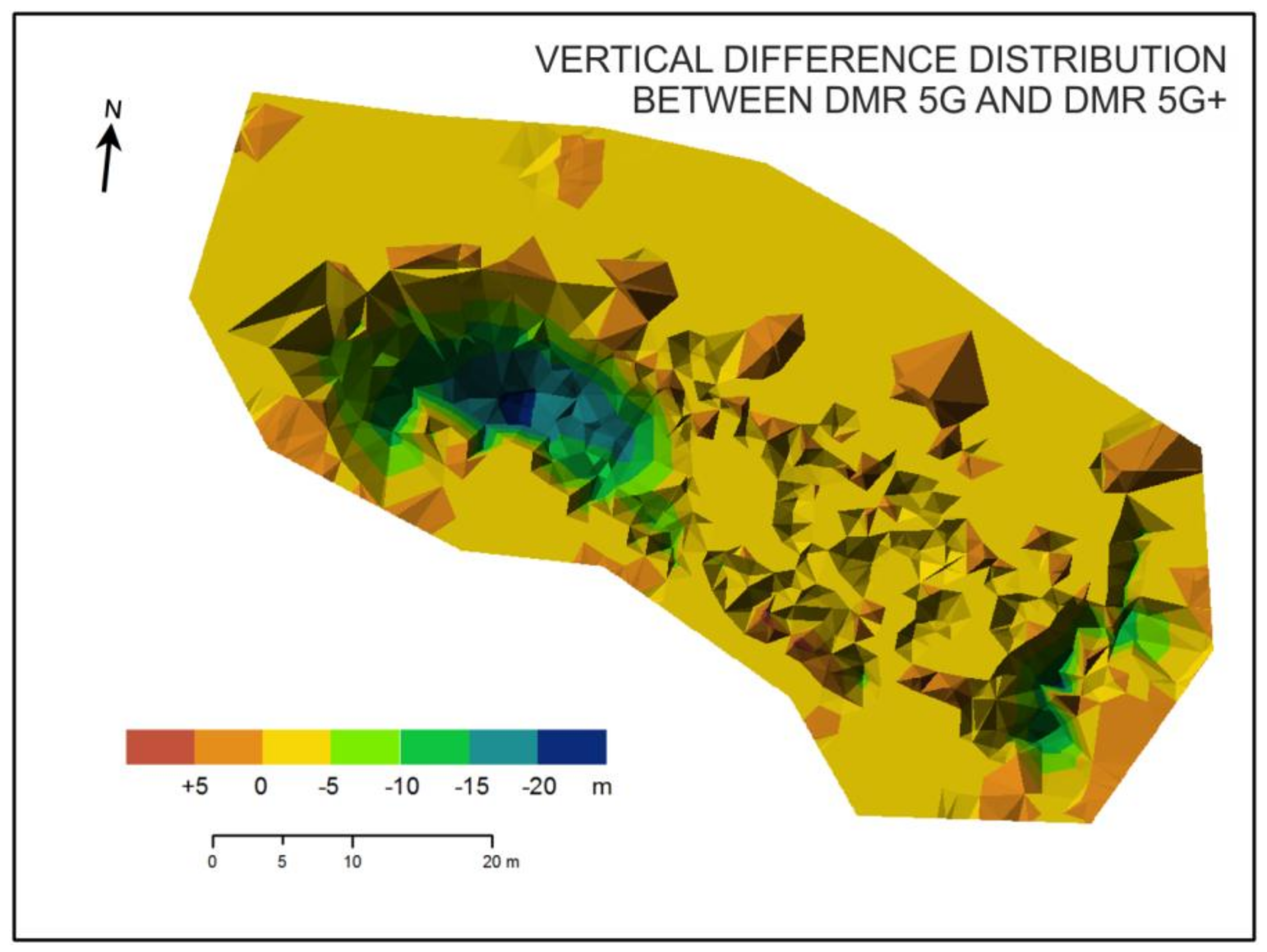
The accuracy of a DMR can be assessed in different ways. The first method applied is the previously used volume difference method (Section 4.1). In this case, the purpose of the method was to define areas of different heights rather than looking for systematic or gross errors. Since the point density of airborne laser-scanning data is much lower at this location, the point cloud over the area bounded by the orthogonal projection of the 3D model was recalculated with additional points. A point network was generated with a 10 cm spacing (equivalent to the average distance of the closest neighbors of 3D-model points) and was interpolated with a height from the triangle-based model created from DMR 5G. At the same time, the 3D model was converted into a triangle-based model in 2.5D.

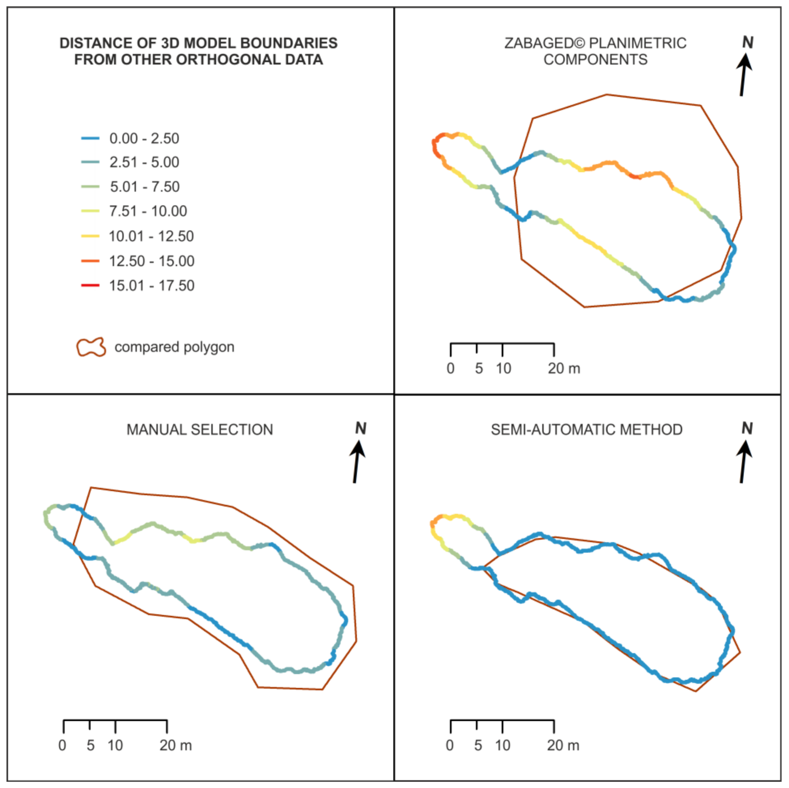
The second way is to assess the orthogonal projection of the rock formation on the map. The orthogonal projection of a 3D model onto a plane lacks information about possible overhangs, but the airborne laser-scanning method works on the same principle. Two possible approaches can be used. The first and less appropriate is the percentage calculation of the area overlapping compared polygons. The second approach works with the distance of the outlines of the compared polygons. The distance can be determined in several ways—searching for the closest neighbor, finding a perpendicular distance to the second outline, or measurement in normal direction (M3C2) between compared polygons. Each of these methods returns numbers in the results which are a little bit different, but their crucial advantage over the first approach is the ability to determine the distance of each part of the compared geometry. A comparison was made here based on the vertices of the boundary line and searching for the closest neighbor. The boundary line of the rock formations created by the semi-automatic method and the horizontal boundary line in ZABAGED^® were densified by vertices with a spacing of 10 cm. Subsequently, the nearest neighbors were found and the minimum distances to the line points (1542 in total) of the orthogonal projection of the 3D rock model were calculated. Both methods were processed in ArcGIS 10.2.2.

The third way to evaluate the quality of DMR models is by the total distance of their points from the nearest neighbors of the point cloud forming the rock’s 3D model. This simple and relatively fast method is used to describe the basic total distance of the compared point data when using the local terrain model [30]. The distance of point clouds was calculated in CloudCompare 2.6.3, with an area of 5 m set to calculate the local model. The result is a spatial distance of clouds which can be decomposed into X, Y, Z coordinates of parallel coordinate system axes.

5. Evaluation of Results

The results of the DMR 5G accuracy assessment need to be seen in the context of previous works. These contributions revealed the influence of low vegetation or permanent grass in fields where the height of recorded points is overestimated by a root-mean-square error of up to 21 cm [22]. In another case, it was found that the altimetry (contour model) of ZABAGED^®, which until the time of airborne laser scanning was the most accurate altimetric database in the Czech Republic, is stored 23 cm higher than in DMR 5G [1]. This was also confirmed with regard to geodetically measured points [25]. However, it is expected that the DMR 5G point cloud does not cover the local maximum and minimum, hence the top of rock formations will show a lower altitude than the densely-represented DMR 5G+ and 3D model from terrestrial scanning.

5.1. Results of DMR 5G Quality Evaluation for the Selected Location

As a starting point where the semi-automatic method of searching for rock formations was applied, the type of object in ZABAGED^® called “Woodland with trees” with code 6.07 was chosen. Selected outliers were linked to polygons with the following settings: maximum point distance of 5 m, maximum distance of 15 m between close polygons, and removal of polygons smaller than 50 m². These settings result from empirical testing of the options above in the underlying data of topographical maps and orthophotos. The result of the process can be seen in Figure 6 showing a comparison of the manual method and the definition in ZABAGED^®. A particularly brief definition of the number of objects is in ZABAGED^®. Airborne laser-scanning data are, therefore, a very good source for updating this database.

When comparing DMR 5G and DMR 5G+ models,

Table 1. Calculated characteristics by volume difference of DMR 5G and DMR 5G+ (absolute error as m_h, systematic errors s_h, gross error as a triple of the standard deviation between elevations of both models).

Area	${\mathit{s}}_{\mathit{h}}$ (m)	${\mathit{m}}_{\mathit{h}}$ (m)	Standard Deviation (m)	Minimum Vertical Difference (m)	Maximum Vertical Difference (m)	Gross Error (m)	Gross Error Rate in Area (%)	Total Area (m2)
Whole area	0.00	0.01	0.17	−21.42	8.38	0.04	1.83	25 × 106
Manual method	−0.81	1.25	2.21	−21.42	8.38	3.76	3.93	47,778
Semi-automatic method	−1.53	2.24	3.18	−21.42	8.38	6.71	8.07	26,769

observes that quite large maximum and minimum vertical differences are at these locations. At the same time, it is possible to observe the increasing altitude variance of the models, an increase in gross errors, and the area they are in together with a gradually decreasing delimitation area of rock formations (Figure 5, Table 1), which indicates the fact that the altitudes of rock formations in the basic model of DMR 5G are underestimated and that higher elevation differences are not only likely to occur on the slopes of rocks, but on peaks. Particularly interesting information is that 8.07% of the area exceeds its inaccuracy of the gross error height of 6.71 m from the reference surface, which is a very high value for the study of visibility or for signal propagation in telecommunications. Therefore, data were collected from the selected rock formation to corroborate or disprove the hypothesis that higher error values are present for the top parts of rock formations.

5.2. Results of the DMR 5G Quality Assessment at Selected Rock Formation

Based on the results above (Section 5.1) and in accordance with the established methodology (Section 4.2), three ways of assessing the accuracy of DMR 5G and DMR 5G+ were proposed against the 3D model itself or its derivations. The vertical difference of both models at this site is shown in Figure 7. In the figure, the DMR 5G model has more or less two error distributions, where the western and south-western part of the rock space is significantly lower (less than −6 m), while the remaining part has an average of 0 to 2 m above the reference model.

The results of the first evaluation method using volume difference applied to a relatively large area set by manual selection in Section 4.1 can be seen in Figure 8. Errors in the north-western part are associated with removing the entire lower block of the rock, so the vertical difference in those areas reaches the highest values. Similarly, vertical differences are visible on the south-western part at the edge of the rock with a slightly overhanging wall. The numerical representation of airborne laser-scanning models and the derived 3D model from terrestrial scanning is shown in

Table 2. Summary data on vertical difference of compared DMR models to the reference model created from the Bílá skála 3D object.

Elevation Model	Mean Vertical Difference (m)	Standard Deviation (m)	Maximum Vertical Difference (m)	Minimum Vertical Difference (m)
DMR 5G	−3.26	5.61	10.21	−20.96
DMR 5G+	−0.82	3.59	21.13	−20.93

.

In addition to extremes in the form of maximum and minimum errors, an important average difference in heights of points is indicated. The value of −3.26 m (negative value means underestimation compared to a real surface) correlates with the observation of vertical differences in Figure 8. By contrast, DMR 5G+ shows that even in the southeastern part of the rock formation some points are captured and not only present in the commercial version of DMR 5G. However, the height deviation in these places is still higher, indicating a probable measurement error.

The results of the second method, which evaluates the position of a rock object in 2D, are shown in

Table 3. Basic parameters of 3D rock object layout, ZABAGED^® planimetric components, manual selection, and semi-automatic method (RMSE means root mean square error).

Type of Method	RMSE (m)	Standard Deviation (m)	Maximum Vertical Difference (m)
ZABAGED® plan. comp.	7.16	4.8	17.01
Manual selection	3.83	1.88	9.07
Semi-automatic method	2.09	3.30	13.18

and Figure 9. These outputs show an inaccuracy in the DMR 5G+ model from which the polygons of rocks were formed, as mentioned in Section 4.1. The outputs indicate high maximum deviations associated with a failure to capture the rock surface area in the north-western part. Based on further processing, DMR 5G is even more generalized in terms of dimensions in the north-western part compared to DMR 5G+ in terms of higher altitude deviations.

The last method of evaluation focused on the total distance of point clouds. Basic error statistics from M3C2 for all axes for both evaluated DMR models are shown in

Table 4. Distances of DMR 5G and DMR 5G+ models with single-axis distribution calculated from a comparison of closest neighbors of point cloud models (RMSE means root mean square error) (m).

Elevation Model	Axis Direction	RMSE (m)	Standard Deviation (m)	Maximum (m)
DMR 5G	X	0.36	0.47	3.44
	Y	0.55	0.70	4.25
	Z	0.36	0.47	3.31
	Total distance	0.81	0.88	4.53
DMR 5G+	X	0.22	0.31	2.67
	Y	0.29	0.39	2.88
	Z	0.24	0.35	3.04
	Total distance	0.47	0.54	3.72

. The options included the neighborhood dimension in which the local relief was calculated and the maximum distance determined. Neighborhood size was calculated as the average of the absolute mean values in the 2D model (Table 3, semi-automatic method) and the vertical difference of the DMR 5G+ model (Table 2). The maximum distance where points were included in the computing process was set at 5 m. The occurrence of individual problematic areas is shown in Figure 10. DMR 5G shows the greatest variation in the middle section of the object, where the highest vertical difference compared to the created 2.5D rock model was observed. The distances in the model from the real surface is on average 0.81 m, with the smallest error components being the X and Z axes, while the Y axis adds maximum distance. The surface of DMR 5G+ shows a difference in surface improvement roughly twice larger regarding distance compared to DMR 5G. These results indicate a lower amount of mass compared to the model from terrestrial laser scanning. Two areas of greater vertical differences can be identified in the model, the first being located on the northern side of the rock surface and the other on the very edge of the studied area in the south-western part.

6. Discussion

The first important result of this contribution is the relatively reliable ability to search for rock formations using the semi-automatic method. Thanks to this method, a rock formation called Černá skála (70 m long, 15 m high, 25 m wide) was found, which is frequently visited by rock climbers and completely missing in the ZABAGED^® planimetric components. This method can help to update it. The method is, however, partly experimental and depends on available data, and therefore it would be useful to test it on a different type of relief and data.

In addition, an altimetric assessment was performed using the volume difference method. This method has already been successfully tested in other parts of the Czech Republic. This paper proved that general evaluation hides errors present in the models, where increasing deformations and the convexity of shapes leads to higher deviations in the vertical geometry of the tested models. This can be seen from the data in Table 1, where the systematic error s_h is zero in the whole available area, while in the assessment of the rock formations it is more than 1.5 m. This finding involved acquiring support data from a terrestrial laser scanner and creating a detailed 3D model of Bílá skála. This three-level assessment on the object showed that both the ZABAGED^® planimetric components and the DMR data did not accurately reflect the north-western block of the rock formation. In the ZABAGED^® planimetric components, a maximum horizontal error of up to 17.5 m is evident. It was also found that the DMR 5G+ data are of higher quality for the top of the rocks, where their average difference is 0.82 m compared to DMR 5G, where the average difference was recorded to reach 3.26 m. This was also investigated from the point of view of the distance between the walls in all axes of the space. DMR 5G+ is approximately 47 cm further away from the real walls of the Bílá skála formation.

One of the factors that can influence the results when assessing accuracy is the location itself. The area is covered with coniferous forests, which can cause problems for both airborne laser scanning [34,35] (for various reasons including poor beam penetration, beam width at impact, and multipath) and terrestrial scanning, where the 3D model needed to deal with rocks occasionally obscured by tree trunks. Another drawback of the 3D model is partial interpolation in the flat top part. Although this site is at most 3–5 m wide, the beam from the terrestrial scanner is unable to reach it and may cause a height deviation of several tens of cm. A partially contentious issue may be in assessing the total distance of rock walls. The method determines the distance based on the distance from the local plane of the relief, which is calculated from the interlacing of neighboring points by a straight line. At the top parts, points can even be selected on the opposite wall, which changes the orientation of the local plane of the relief, and an incorrect value is entered into the result of the test point.

It is obvious that the current quality of the DMR 5G model in areas with rock formations has certain drawbacks. Obtaining better quality for the top of rock formations must necessarily involve several successive steps. Experimentally, it was found that the current density of points (even with respect to raw data) for the identification and more precise spatial delimitation of rock objects is insufficient [10]. As the minimum point density, the 10 p/m² limit is fixed and scanning from different directions to deal with obstructions is recommended. This recommendation can be further extended to the parameters of a flight plan and its components. For example, it would be necessary to provide better beam penetration through the vegetation layer when scanning during the vegetative season, such as reducing the flight level of the aircraft, increasing the transmitted beam intensity, or reducing the beam view angle so that the final achieved density corresponds to the set plan. By contrast, the experience of [36] suggests that even higher point density may not always guarantee a more accurate result. At a density of 7 p/m², boulders with a base size of at least 4–6 m can be clearly identified. But it is still unlikely to solve the issue of overhangs, which are more conveniently scanned with other methods (such as terrestrial station, remote-piloted aircraft systems). This method for processing supplementary data would be possible even under difficult situations as shown in [12]. One possible error in testing and modeling the Bílá skála object is the varying point cloud density. In the next stage of the research, this could be reworked into a better model, but the cost would be increased calculation time [12].

By comparing the results with [11] it can be argued that one of the most important parameters in searching for rock outcrops and formations is slope, while altitude or slope orientation is not so important. By contrast, the method of volume difference with a triangle-based structure is more credible than raster representation [11,24] for calculating the volume of displaced mass. If the required final cloud density is met, additional support steps must be taken to improve the classification of points in groups such as vegetation and terrain to avoid undesirable errors. One of the options is to process additional information about the return beam. If information from a scanner is available, such as the width or intensity of the returned pulse, this information can be used as support for other parts of the processing steps. Calculating the ratio between the width and amplitude of the returned pulse proposed by [10] and the consequent derivation of the probability characteristics of each point in a group appears to be a usable parameter in this case. However, it is based on the simple behavior of the beam, which in fact has more complex interactions with the surrounding environment. For this reason, other variables, such as information about the physical condition of objects, should be included in the characteristics if available. Another option is to create several groups of certain types of objects that can serve as training surfaces to derive the necessary characteristics of the reflected signal. Based on these characteristics, the return signal may be decomposed. In the case of existing manual classification based primarily on evaluating the geometric information of points, the success in leaving terrain points in rock formations may increase together with the time needed for the manual processing phase. It is likely that the ratio of poorly assigned points to other groups would be reduced.

The results obtained should have a primary impact on the processing steps of ALS data. If the points above problematic sites are added, DRM 5G will achieve other possible and higher-quality uses. This should be directly reflected in cartographic production when updating the ground-level definition of rock formations, which will certainly be found in hiking maps. Up-to-date altitude information will improve the visibility modeling methods for an area, as long-term plans to increase the attractiveness of an area are calculated taking into account the ongoing deforestation of rock formations. An undeniable advantage would be gained from the use of DMP 1G in saving some of the nearby tree vegetation in the vicinity of the rocks.

7. Conclusions

This paper deals with processing and evaluating DMR digital terrain models aimed at identification of rock formations. The introduction presents the derived models under a project in the Czech Republic for creating new altimetry and their declared quality. In addition, theoretical concepts of laser-scanning errors are presented. The main content of the paper is divided into two parts. The first part includes a semi-automatic method to identify rock formations from a point cloud. These objects are then assessed for accuracy using the volume difference method between DMR 5G and DMR 5G+ data. Based on the preliminary results, support data was collected on the selected rock formation Bílá skála using terrestrial laser scanning. A faithful 3D model of the object was created and used for a more accurate three-level evaluation of the quality of the relief digital models. The results showed that the quality of the DMR 5G model decreased with increasing fragmentation and relative height of the rock formation, while the proportion of gross errors increased. The complementary DMR 5G+ is better in terms of location and altitude but has occasional fundamental errors. Finally, the steps for evaluation and the possible future development of data are critically discussed.

Currently, alternative methods for stereophotogrammetric evaluation of data sources originating from piloted or remotely controlled aircraft systems (RPAS) are being developed. These systems offer greater operational space and faster data processing and evaluation. However, they fail to map hidden objects and situations that are not possible to capture with photos. Therefore, regarding the further development of mapping, it will be important to complement and use adequate data for the specific needs of a project. As usual, emphasis should be placed on quality, not quantity. Airborne laser-scanning data have a certain quality because of the objectives of the project, but it is necessary to think about them in a different way rather than through their declared overall reliability.