Analyzing and Predicting Micro-Location Patterns of Software Firms

Abstract

While the effects of non-geographic aggregation on statistical inference are well studied in economics, research on the effects of geographic aggregation on regression analysis is rather scarce. This knowledge gap, together with the use of aggregated spatial units in previous firm location studies, results in a lack of understanding of firm location determinants at the microgeographic level. Suitable data for microgeographic location analysis has become available only recently through the emergence of Volunteered Geographic Information (VGI), especially the OpenStreetMap (OSM) project, and the increasing availability of official (open) geodata. In this paper, we use a comprehensive dataset of three million street-level geocoded firm observations to explore the location pattern of software firms in an Exploratory Spatial Data Analysis (ESDA). Based on the ESDA results, we develop a software firm location prediction model using Poisson regression and OSM data. Our findings offer novel insights into the mode of operation of the Modifiable Areal Unit Problem (MAUP) in the context of a microgeographic location analysis: We find that non-aggregated data can be used to detect information on location determinants, which are superimposed when aggregated spatial units are analyzed, and that some findings of previous firm location studies are not robust at the microgeographic level. However, we also conclude that the lack of high-resolution geodata on socio-economic population characteristics causes systematic prediction errors, especially in cities with diverse and segregated populations.

1. Introduction

The location pattern of any industry is the product of a large number of individual decisions. Industrial location analysis investigates these location decisions and seeks to detect location determinants that trigger and influence such decisions. These determinants are generally referred to as location factors. A thorough understanding of the impact of location factors on firms’ location decisions and firm performance can have important implications for stakeholders. Managers and entrepreneurs can integrate valuable information into the decision making process when choosing the location of a new venture [1].

Policy makers at the regional, national, and multinational level want to promote economic growth by developing the right location factors to create a beneficial environment for firms. The long-standing study of industrial location research [2] has brought forward a wide range of location factors which can be studied at different levels of geographic aggregation, from the immediate firm neighborhood to highly aggregated spatial units. However, the analyzed location factors may vary in direction and strength at different levels of analysis and findings from aggregated spatial vary depending on the spatial scale at which the analysis is conducted [3]. This issue is generally referred to as the Modifiable Areal Unit Problem (MAUP), which is defined through a location, a scale and a shape dimension [4,5,6]. The selection of the appropriate level of analysis is therefore crucial, especially in studies which evaluate public policies [7,8], and must be based on reasonable and transparent assumptions.

Such assumptions rely on a thorough understanding of geographic aggregation effects on statistical inference. While the effects of non-geographic aggregation on inference are well studied in economics [9,10], research on geographic aggregation is rather scarce. Amrhein [11] finds that scaling has strong effects on regression coefficients and correlation statistics. However, it is unclear how robust these results are in an empirical setting as simulated data was used in this study. Arauzo-Carod et al. [12] and Manjon-Antolin et al. [13] find only minimal zonation effects on regression results. Briant et al. [14] use administrative spatial units and gridding to assess both the scaling and shape dimension of the MAUP. They find that the use of different spatial units results in different regression coefficients. Overall, the understanding of the MAUP in industrial location analysis remains incomplete and Arauzo-Carod et al. conclude in their meta-study on industrial location research that “[…] the reported effects may not be robust to the use of alternative geographical units and the presence of spatial effects. In general, it is not clear what effects spatial aggregation and spatial dependence may have on the inference” [15]. Most previous studies analyzed firm location patterns aggregated at rather crude spatial scales, such as counties or metropolitan areas, and thus there is a lack of understanding of location determinants at the microgeographic level. The varying direction and strength of location factors at different levels of aggregation may lead to superimposed location factors which are missed when aggregated geographic units are analyses. Some location factor-firm relationships which are relevant at the macro level (aggregate) may not be so at the micro level (ecological fallacy).

Suitable data for such a microgeographic analysis has become available only recently through the emergence of Volunteered Geographic Information (VGI) [16] and the increasing availability of official (open) geodata [17,18,19]. The OpenStreetMap (OSM) project is of particular interest in the context of firm location analysis as it goes beyond mapping ordinary road networks: The informal OSM standard contains hundreds of tags in over 25 categories and includes map features such as amenities and public transport stations [20]. Up to now, only few studies have utilized the potential of OSM in firm location analysis and geographic economic analysis in general [21,22,23]. However, these studies did not use OSM in a large-scale spatial analysis but concentrated on single cities and a strongly limited set of location factors. Following the analysis of previous research efforts, the research questions for our work are defined as follows:

RQ1

Are the effects of location factors, as reported by previous studies using aggregated spatial units, robust at the microgeographic level?

RQ2

How does a firm location prediction model perform at the microgeographic level and to what degree does it provide valuable new insights into the firm allocation process? What are the distinct requirements to the data and the statistical model?

To answer the research questions above, we analyze firm location patterns at the microgeographic level using spatial firm-related data that are available in unseen detail compared to previous studies. We combine this unique data set of three million geocoded street-level firm observations in Germany with OSM data and other detailed geodata (population density, land cover, railway stations, education levels, life expectancy, and many others). We investigate whether findings from previous industrial location studies hold true at a small spatial scale, i.e., at fine spatial resolutions. In general, regular gridding reduces the bias induced by the use of predefined administrative units [24]. In our study, we focus on the software industry, which is rather unrestricted in its location decisions [22], inducing only little bias from unobservable location determinants.

First, we investigate the software firm location pattern in an Exploratory Spatial Data Analysis (ESDA). We find that Poisson regression is likely to be an appropriate method to model the pattern of software firms aggregated at a regular 1 km grid, whereas negative binomial regression seems to be appropriate for higher levels of aggregation due to over-dispersion in the point pattern. Further, we find that software firms are an urban phenomenon, as they are disproportionally frequent in and around urban areas and even form statistically significant hotspots in some city regions. We further conclude that the regional settlement structure (polycentric vs. monocentric) seems to have an impact on the location pattern of software firms.

In a consecutive step, we construct a Poisson regression model to predict the number of software firms per 1 km grid cell using a large set of location factors. In the regression analysis, we include 24 different agglomerations, infrastructure, socio-economic, topographical, and amenity location factors. We interpret the estimated regression coefficients to deduce the relationships between the location factors and software firm counts. Due to identification limitations [25,26] in our model, we abstain from tagging causal relationships and rather concentrate on the predictive performance of our model. However, by comparing our estimates with estimates from previous studies, we are able to discuss differences in the location factor-firm count relationships at different levels of geographic aggregation. We find that our model’s overall performance is good as it is able to redraw the software firm pattern to a high degree and yields reasonable coefficients, which are in line with prior research. Inter alia, we are able to show that regional population centrality (which we operationalize using the Urban Centrality Index [27]) is a significant predictor of local software firm numbers at the microgeographic level. However, we also find that our model has a weak performance in highly segregated cities with quarters characterized by populations with dissimilar socio-economic profiles. Due to data limitations, we are not able to capture this microgeographic heterogeneity in the population structure. When considered at the aggregate city level (25 km grid), this systematic prediction error is levelled and the model yields systematic (spatially autocorrelated) errors in areas which were identified as software industry hotspots in the ESDA. This indicates that our model specification misses some crucial location factors present in these areas or some of the model’s assumption are violated (e.g., the independence between individual location choices).

2. Data

In this study, we utilize geographic data from three main sources: The OpenStreetMap project, official geodata from statistics agencies, and the geocoded Mannheim Enterprise Panel dataset.

2.1. OpenStreetMap Data

OpenStreetMap (OSM) is a collaborative mapping project, which allows users to create freely accessible geographic data. In addition to roads, OSM includes map features such as retail shops, public transport facilities, and a variety of natural features. Concerns about the quality of this kind of user-generated geographic information seem natural and emerged shortly after the launch of the project in 2004 [28]. An array of studies investigated OSM data and assessed the geometric, attributive and temporal accuracy, and completeness of the mapped features. Besides intrinsic approaches, most of these studies compare OSM data to established commercial or official geographic data on road networks [29,30,31], buildings [32], and land use data [33,34,35]. Their results show, first, that OSM data is only slightly inferior to official/commercial data in terms of accuracy. Second, OSM data completeness increases at a rapid rate and is assumed to have reached or exceeded the level of completeness of commercial data in the meantime. Third, the completeness of OSM is positively correlated to population density and can be considered to be particularly suitable for the spatial analysis of urban areas. In this study, we use motorway accesses, airport locations, public transport stops, and several types of amenities obtained from an unmodified OSM full copy [20]. We also use OSM geodata as base data for our address locator described below.

2.2. Official Geodata

We use data issued by several German and European agencies, such as a downscaled population density grid issued by the European Environment Agency, which is available in 100 m resolution and is based on communal census population data and land cover data (CORINE and LUCAS) [36]. Further, we use data on intercity railway stations and a 200 m resolution digital elevation model obtained from the German Federal Agency of Cartography and Geodesy. Socio-economic data on the level of education of the local workforce, wages, life expectancy, and number of resident students were obtained from the German Federal Institute for Research on Building, Urban Affairs and Spatial Development. Crime data was obtained from the German Federal Criminal Police Office. Due to the high data privacy awareness in Germany, the utilized socioeconomic data are only available at the municipality or district level. Local business tax rates were obtained from the German Federal Statistical Office. Local high speed broadband Internet availabilities are based on data from the German Federal Ministry of Transport and Digital Infrastructure. Locations of research institutes and universities were obtained from the German Federal Ministry of Education and Research. A 1 km resolution grid with the average commercial rent per square meter in 2016 was provided by the data company empirica-systeme GmbH, Berlin, Germany.

2.3. The Mannheim Enterprise Panel

The Mannheim Enterprise Panel (MUP) is a firm data base which covers the total stock of firms located in Germany. It contains about three million firm observations which are updated on a semi-annual basis. The data covers firm characteristics such as the branch of industry through NACE codes (a classification of economic activities in the European Union) and postal addresses [37]. Our definition of the software industry (the used NACE codes are: 62.01.0, 62.01.1, 62.01.9, 62.02.0, 62.03.0, 62.09.0, 63.11.0, 63.12.0) covers general programming activities, software development, web portals, data processing, and the development of web pages. In 2016, the MUP contained about 2.97 million active firms in Germany of which 70,009 are software firms (2.36%). We geocoded all MUP firm addresses using a self-made street type geocoding address locator based on an extended street network data model without house number interpolation. The geocoding results were assessed concerning their completeness and positional accuracy as proposed by Zandbergen [38].

The geocoding resulted in a completeness of 95.2% for the overall data set and 97.8% for the software firm subgroup in particular. The positional accuracy was verified by geocoding a random sample (n = 1000) of successfully geocoded addresses using a conventional geocoding service. The median positional offset between our geocoding results and the results obtained from the conventional service is 58 m (95% confidence interval: 53–69 m) and the mean is 252 m (95% confidence interval: 210–295 m), which is suitable for our level of analysis. A further analysis of the spatial distribution of the geocoding match rate aggregated at postal code areas revealed significant clustering (Moran’s I = 0.13, *** p < 0.001) with few significant local clustering (Getis-Ord G_i*) of low match rates in rural areas. However, there is only a minor positive correlation (r_s = 0.006 ***) between the geocoding match rate and population density. Hence, known OSM data quality issues in rural areas (see above) do not seem to induce a systematic error in our geocoding results. We included an according control variable in the regression analysis (geocoding match rate at postal code area level) to cope with spatially varying geocoding completeness. We further used the MUP to identify the headquarter locations of the top 100 firms (by annual turnover) in Germany to include them as a location factor in the regression analysis.

3. Methods

Our analysis of the software firm location pattern is based on Exploratory Spatial Data Analysis (ESDA) and count data regression analysis.

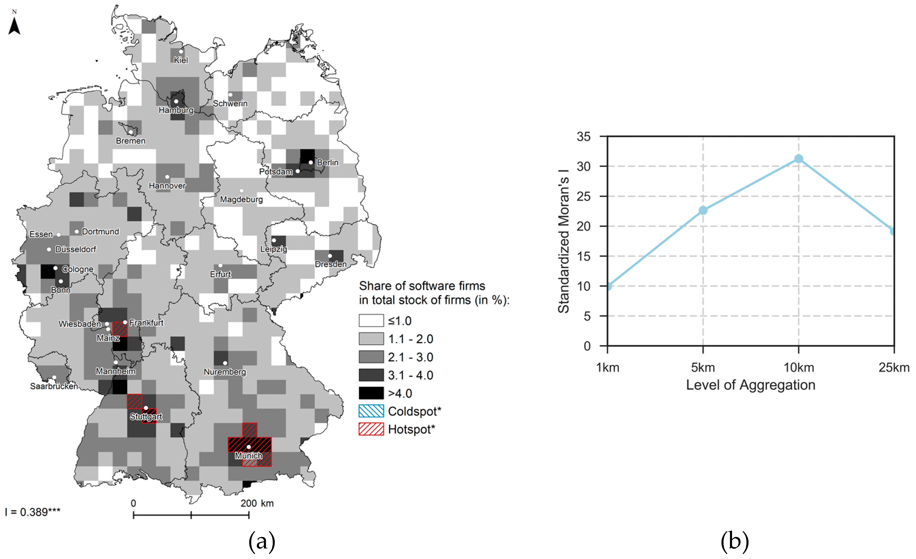
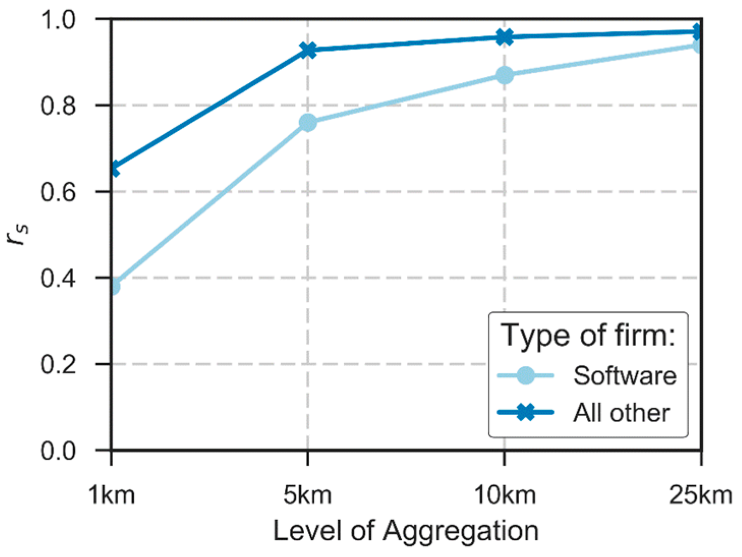
3.1. Exploratory Spatial Data Analysis

Exploratory Spatial Data Analysis is a general term to describe the analysis of geospatial data in an explorative manner using a wide range of methods. It is similar to Geographic Knowledge Discovery [39], Spatiotemporal Data Mining [40], and GeoVisual Analytics [41,42]: Unexplored data is analyzed with the objective to uncover relevant and significant data characteristics or relationships (e.g., data patterns, trends, correlations). Furthermore, the results should be summarized in an easily understandable way.

In this study, graphical techniques and geovisualization [43] are used to display and explore geographic data. Correlation analysis is used to measure the direction and strength of association between pairs of variables. We use the non-parametric Spearman’s rank correlation coefficient r_s to measure the degree of monotonic relationship between variables. Quadrat analysis is used to evaluate the dispersion of point patterns by calculating their variance-to-mean ratio (VMR) using regular grids. The results of the quadrat analysis are used to assess whether the software firm location point pattern was produced by a random (homogenous Poisson) process [44,45]. We measure global spatial autocorrelation using Moran’s Index I, which is arguably the most common measure to do so. We also utilize standardized Moran’s I z-values, which allow us to compare I values between different levels of spatial aggregation. The generalized local G autocorrelation statistic G_i* is used to evaluate local spatial association [46]. G_i* was selected because we are mostly interested in detecting local pockets of positive spatial autocorrelation (e.g., “hotspots of the software industry”). Measures of spatial autocorrelation require us to hypothesize the spatial relationships in the study area [47]. We use the topological contiguity method with queen contiguity criterion (QNN) for our regular grids.

3.2. Count Data Regression Models

The most common way to model the relationship between location factors and the number of local firms per areal unit are count data regression models (CDM) [15]. The estimated coefficients from CDM provide evidence on how ceteris paribus variations in an explanatory variable affect the conditional mean of the number of local firm locations. However, it is not advisable to deduce causal relationships between the dependent variable and the explanatory variables without having a suitable identification strategy [26,48]. Relationships estimated in our regression analysis should be understood as correlations between our dependent variable (software firm counts) and a set of predictor variables (location factors).

We apply the most commonly used CDM: Poisson regression [26,49]. In a spatial setting, the data generating process can be understood as a spatial Poisson process. The standard (homogenous) spatial Poisson process generates points with complete spatial randomness (CSR) [44]. Spatial Poisson processes are used in many fields to model randomly distributed points [45,50]. An outcome Y is assumed to be Poisson distributed with a stationary density parameter λ. This density parameter defines both the mean and the variance of the distribution (equidispersion). A point pattern which features a spatially varying density parameter λ can be understood as a non-homogenous Poisson process. Here, the outcome Y depends on a location-dependent density parameter λ that varies systematically with a set of variables X (i.e., the location factors).

Y ~ Poisson(λ(X)) E(Y) = λ(X) Var = λ(X)

(1)

Hence, the local density parameter λ_i in cell i is conditional on the local values of x_i:

y_i|x_i ~ Poisson(λ_i) E(y_i|x_i) = λ_i Var_i = λ_i

(2)

The effect of X on Y is defined by a set of unknown coefficients. These coefficients can be estimated in a Poisson regression, which is a generalized linear model with the natural logarithm as the link function. The parameter estimation is based on maximum likelihood. The expected count (i.e., the number of firms) in an area i of size A_i, given n location factors x, is then:

$${\widehat{\mathrm{y}}}_{\mathrm{i}}=\widehat{{\mathsf{\lambda }}_{\mathrm{i}}}={\mathrm{e}}^{\ln ({\mathrm{A}}_{\mathrm{i}})+\widehat{\mathsf{\alpha }}+\widehat{{\mathsf{\beta }}_1}{\mathrm{x}}_{1,\mathrm{i}}+\dots +\widehat{{\mathsf{\beta }}_{\mathrm{n}}}{\mathrm{x}}_{\mathrm{n},\mathrm{i}}}$$

(3)

The coefficient exp(α̂) is the offset, while exp($\widehat{\mathsf{\beta }}$) give the multiplicative effects of the location factors. The estimated coefficients can be reported as incidence-rate ratios (IRR) which make comparing rates easier. The IRR for a Δx_n change in x_n is ${\mathrm{e}}^{{\widehat{\mathsf{\beta }}}_{\mathrm{n}}\Delta {\mathrm{x}}_{\mathrm{n}}}$ (ceteris paribus). Cameron and Trivedi [26] recommend using robust standard errors for Poisson models.

We also use Negative Binomial regression (NBIN), which is a special case of Poisson regression [49]. In NBIN regression, it is assumed that an overdispersed Poisson process generated the point pattern under investigation. To cope with the additional variance, an additional shape parameter (over-dispersion parameter) is estimated, which allows for additional variance [26].

4. Results

In this section, we first present the results of our Exploratory Spatial Data Analysis (ESDA). Building on our findings from the ESDA, we construct a comprehensive set of location factors, which we use in a subsequent regression analysis. The results of the regression analysis are presented in the second part of this section. A detailed discussion of the results and their significance follows in Section 5.

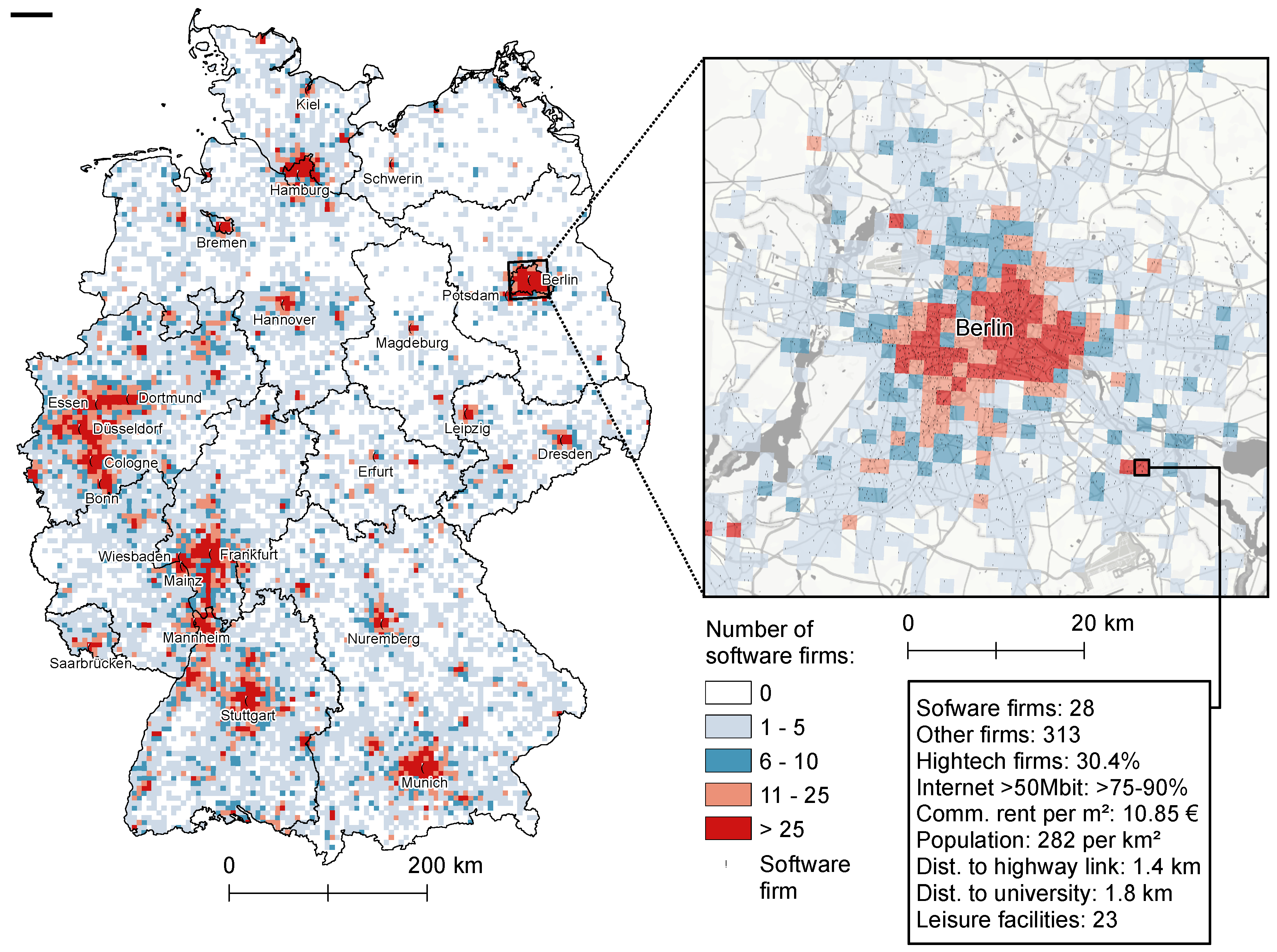
4.1. Exploratory Spatial Data Analysis Results

Table 1. Descriptive statistics of the aggregated software firm location pattern.

Scale	Obs.	$\overline{\mathbf{X}}$	$\tilde{\mathbf{X}}$	SD	Min.	Max.	VMR	Histogram
1 km	361,453	0.19	0	1.64	0	211	14.12
5 km	14,951	4.58	1	25.98	0	1604	147.39
10 km	3860	17.74	4	87.07	0	3265	427.35
25 km	671	102.06	27	301.74	0	4105	892.11

Histogram: x = number of firms per cell; y = frequency.

presents descriptive statistics of the software firm pattern aggregated at 1 km, 5 km, 10 km, and 25 km resolution grids. It can be seen that the variance-to-mean ratio (VMR) of the distribution strongly varies with the level of aggregation. At low levels of aggregation, the distribution is closer to equidispersion (indicating that the point generating process can be adequately modelled as a Poisson process). At higher levels of aggregation, the pattern appears to be increasingly clustered (over-dispersed). We conclude that Poisson regression is likely to be the appropriate regression model for low aggregation levels, while Negative Binomial regression, which can handle over-dispersed count data [49], seems to be more appropriate for higher levels of aggregation. These results show that the choice of level of aggregation highly influences the statistical characteristics of the spatial pattern under investigation and determines the choice of an appropriate statistical distribution.

Figure 1 maps the gridded distribution of software firms in Germany. An exemplary focus map of the German capital Berlin is shown to give an impression of the data’s level of detail. It can be seen that the pattern largely redraws the population distribution: High numbers of software firms can be found in and around urban areas and low numbers in less densely populated areas. It is well known that the geographic pattern of economic activity is dominated by the influence of the population distribution: Humans tend to concentrate in specific areas, causing a high frequency of firm locations in those areas regardless of other factors. The population density can therefore be considered the reference pattern of the firm location distribution.

However, Figure 2a indicates that software firms seem to have a location decision behavior different from the rest of the firm population. It can be seen that the share of software firms in the overall firm population is not distributed randomly over the study area (Moran’s I = 0.36 ***; the standardized I values plotted in Figure 2b show that this applies to all scales). Instead, software firms are disproportionally frequent in and around urban areas and even form statistically significant (p ≤ 0.05) hotspots (Getis-Ord G_i*) in the areas of Munich, Stuttgart and Rhine-Main (around Frankfurt). On the contrary, the absence of high software industry shares and hotspots in the very densely populated and large Ruhr area (around Essen) indicates that high population density alone does not necessarily imply large proportions of software firms in the local firm population.

Figure 3 helps to further investigate the relationship between firm numbers and population density by plotting Spearman’s correlation coefficients for four levels of geographic aggregation. It can be seen that the positive monotonic relationship becomes stronger with the level of aggregation. Aggregated at 25 km, both software firms (r_s = 0.94 ***) and the total stock of firms (r_s = 0.97 ***) exhibit similarly strong monotonic relationships with population numbers. At the 1 km scale, software firm numbers show a distinctively lower correlation to local population numbers (r_s = 0.38 ***) than the rest of the firm population (r_s = 0.65 ***). This indicates that population numbers alone do not predict the number of software firms very well at low levels of geographic aggregation.

Combining the findings from Figure 2 (large shares of software firms in densely populated areas) and Figure 3 (weaker correlation between software firm numbers and population numbers at the microgeographic level), which seem counterintuitive at first sight, leads us to the hypothesis that software firms do indeed locate in urban regions but prefer the less densely populated areas within cities (e.g., suburbs). Given that the overall firm population is largely dominated by firms from walk-in customer oriented sectors (retail, gastronomy, and personal services) it seems reasonable to assume that these firms seek to locate in the densest areas of cities (i.e., the city center/central business district). Software firms, on the other hand, are not dependent on walk-in customers and may locate disproportionally often in less dense areas, which are usually characterized by lower rents, but still offer most of the benefits of an urban environment. This location choice behavior, which we try to model in the upcoming sub-section, may lead to the observed location pattern of software firms.

4.2. Regression Analysis Results

Based on the findings in the previous section, we specify a comprehensive model that correlates the number of software firms per 1 km grid cell to the values of 24 distinct location factors from five groups: agglomeration, infrastructure, socio-economic, quality of life and amenities, and other location factors. Poisson regression was identified as the appropriate method to model the software location pattern at the 1 km level of aggregation. The location factors and the estimated coefficients yielded by the Poisson regression are given in

Table 2. Location factors and estimated coefficients with robust standard errors in parentheses.

Location Factor	Description	IRR
Agglomeration Location Factors
Firm density	Number of local firms (in 10)	1.028 *** (0.003)
Firm density²	Squared number of local firms (in 10)	0.999 *** (0.000)
High-tech firms	Proportion of high-tech firms in local stock of firms (in %)	1.021 *** (0.000)
Major firms	Distance to next major firm in km	0.998 *** (0.000)
Commercial rent	Difference local rent to mean rent in neighborhood (in Euro)	1.127 *** (0.12)
Population	Population per cell (in 100)	1.081 *** (0.003)
Population²	Squared population per cell (in 100)	0.999 *** (0.000)
Population centrality	Urban Centrality Index (in 0.1 UCI) high value ≙ monocentricity	1.079 *** (0.192)
Infrastructure Location Factors
Broadband Internet	Availability of ≥50 mb Internet (categories) high value ≙ low availability of Internet	0.764 *** (0.009)
Motorway	Distance to nearest motorway access (in km)	0.977 *** (0.001)
Railway	Distance to nearest main-line railway station (in km)	0.998 *** (0.000)
Airport	Distance to nearest main airport (in km)	0.998 *** (0.000)
Public transport	Weighted count of public transport stops	1.000 (0.001)
Socio-economic Location Factors
Wages	Median income of full time employee (in 100 Euro)	1.005 (0.003)
Universities	Distance to nearest university (in km)	0.980 *** (0.000)
Research institutes	Number of research institutes	1.004 (0.036)
Educated workforce	Proportion of graduate employees in %	1.063 ***(0.006)
Students	Proportion of students in local population in %	0.986 *** (0.003)
Business tax	Business tax factor (in 100) high values ≙ high taxes	0.925 ** (0.023)
Quality of Life and Amenities Location Factor
Life expectancy	Mean life expectancy of population	1.092 *** (0.012)
Crime	Violent and street crime incidents per 1000 inhabitants	1.021 (0.015)
Recreation	Number of recreational, community, and sports facilities	1.056 *** (0.008)
Culture	Number of cultural facilities	1.015 0.017
Leisure	Number of gastronomy, nightlife, and general leisure facilities	1.002 (0.002)
Other
Terrain	Difference in elevation to mean neighborhood elevation (in 100m) high values ≙ hillside location	0.919 *** (0.004)
Geocoding control variable	Geocoding match rate (in %) high value ≙ high completeness	1.018 *** (0.002)

** p ≥ 0.01, *** p ≥ 0.001.

. The regression coefficients are given as incidence-rate ratios (IRR) and can be read as follows: An increase in the population by 1 unit (equaling 100 inhabitants) is associated to an 1.081 (+8.1%) times larger number of local software firms and an increase in the distance to the next motorway access by 1 unit (1 km) is associated to an 0.977 (−2.3%) times smaller number of local software firms. The robust standard errors of the estimated coefficients are given in parentheses.

4.2.1. Interpretation of Regression Coefficients

We included the square of both the number of firms and the population to control for a nonlinear relationship with the number of software firms. The reason for taking this approach is because it is frequently stated that density may have an inverse u-shaped influence (an initially positive effect which, from a certain point on, turns into a negative effect, e.g., due to environmental pollution in very dense cities) on site attractiveness [21,51]. This seems to be confirmed by our estimation results. Both the number of firms and the population have a highly significant positive effect on the number of local software firms. The significant negative coefficients of their squared counterparts indicate the assumed inverse u-shaped relationship. Population centrality is also estimated to have a significant effect. Increasing the monocentricity in the regional population distribution leads to an increase in the number of software firms. A high proportion of high-tech firms (classification according to [52]) in the local stock of firms is estimated to increase the number of software firms significantly as well. Increasing distance to major firms is associated to a significant decrease in the number of software firms. Higher commercial rents, expressed as the deviation from the mean rent in the immediate neighborhood (queen contiguity), are estimated to have a positive and significant influence. The model confirms that software firms locate in monocentric and dense areas, but avoid the densest areas. Geographic proximity to business customers (in the form of high-tech and major firms) matter as well. The strong positive effect of high (relative) commercial rents makes it a good predictor. However, there is severe endogeneity stemming from the simultaneity to the dependent variable (attractive locations causing high software firm numbers, which in turn cause high rents), an issue which is addressed in the Discussion section.

Increasing the distance to the motorway, railway, and aerospace network is associated with a significant decrease in the number of software firms. Access to public transport, on the other hand, has no significant effect. Decreasing the availability of broadband Internet is estimated to decrease the number of software firms significantly. These results indicate that software firms prefer locations with decent personal transport infrastructure and available broadband Internet. Local public transport does not seem to be of importance though.

The closeness to a university significantly increases the number of software firms. Counterintuitively, having a high proportion of students in the local population has a significant negative effect. The number of nearby research institutes and wages have no significant effect. Having a high share of graduate employees in the total stock of employees increases the number of software firms significantly, while high business taxes have a significant negative effect. These results indicate that software firms seek to locate close to universities and regions which offer an educated workforce and low business taxes. While this matches the image of the software industry as a knowledge intensive sector, the negative effect of students seems rather implausible. It shall be noted that wages, educated workforce, student population, and business tax levels are measured at a broad geographic scale (counties) and should therefore be understood as regional controls rather than microgeographic predictor variables.

High life expectancy is associated with a significant increase in the number of software firms. The same is true for the number of nearby recreational amenities. Crime rates, cultural amenities, and leisure amenities have no significant effect. These results indicate that a high quality of life does indeed increase the local attractiveness towards knowledge intensive software firms, which heavily rely on highly qualified and creative individuals who are assumed to have a strong preference for areas offering a high quality of living. The breakdown into different amenity types shows that only nearby recreational amenities seem to matter though. However, it should be kept in mind that other amenities could still play a role at different spatial scales: Having a cultural amenity in a city may increase the attractiveness of the city as a whole, but not necessarily the attractiveness of the immediate neighborhood around it.

We included a terrain variable, which captures the difference in elevation between focal cells and their neighborhood. This allows us to distinguish adjacent cells with almost identical location factors (e.g., distance to infrastructure) but different topographies (i.e., hillside location versus valley location). We assume that the identification of hillside location greatly improves the microgeographic predictive performance of our model. The large estimated negative and significant effect supports this assumption. The added geocoding control variable improves the predictive performance as well.

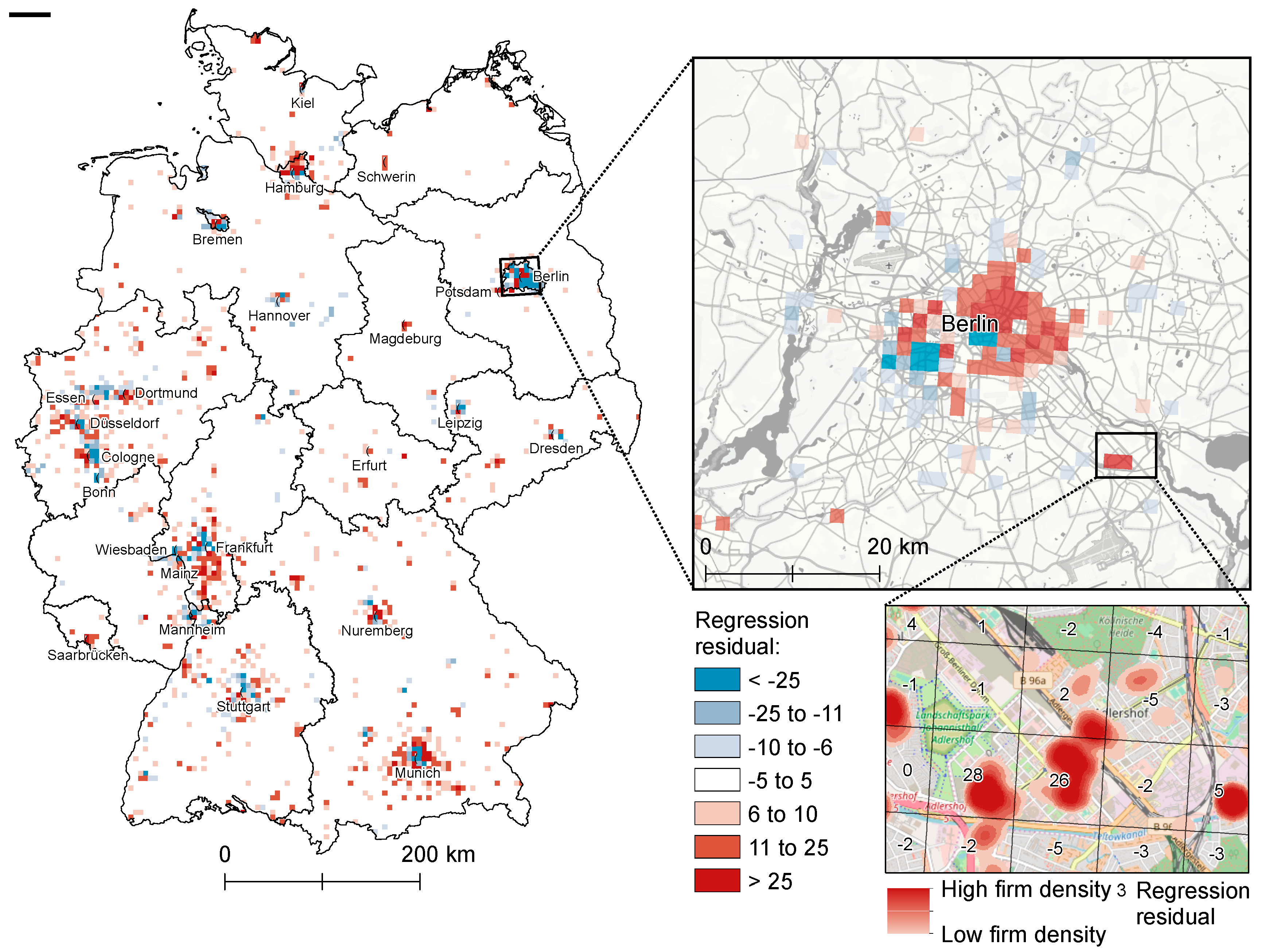
4.2.2. Model Fit and Spatial Residual Analysis

Model fit can be rather difficult to assess and there are a variety of measures of how adequately the model represents the data. We apply different goodness of fit measures (GoF) and spatial residual analysis to assess the fit and adequacy of our model.

Table 3. Poisson and Negative Binomial model goodness of fit.

GoF Measure	Poisson	Negative Binomial
Pseudo-R²	0.58	0.33
RMSE	1.36	483,735
AIC	211,603	179,705
BIC	211,892	180,004

presents some GoF for the model based on the Poisson distribution assumption and the corresponding values from an estimation using Negative Binomial regression (NBIN). The pseudo-R² measures the badness of fit (deviance) of the model, i.e., how much worse the model is than a perfectly fitting model [49], and can only be interpreted against another model’s pseudo-R². According to the root-mean-square error (RMSE) and pseudo-R² measure, the NBIN model’s fit is inferior to the Poisson model. The Akaike Information Criterion (AIC) and the Bayesian Information Criterion (BIC) are widely used measures to support model selection [26,49]. Both indicate that the NBIN model has the better fit (indicated by smaller values), contrary to the RMSE and pseudo-R².

Figure 4 plots the frequencies of observed against predicted software firm counts (as proposed by [26]). It can be seen that the NBIN model yields severely overestimates firm counts. This is reflected by the RMSE but not the AIC and BIC, which are less sensitive towards severe over- and underestimation. In line with our prior assumptions, based on the descriptive statistics in Table 1, the Poisson model seems to be the better prediction model at this scale. However, it can also be seen that both models underestimate the number of zeros and low count cells. This indicates that an excess zero problem might be prevalent in our model. This can be the case if the study area includes areas (i.e., raster cells) that would never host any firms (e.g., water bodies). One way to deal with such structural zeros is to use Zero Inflated Poisson regression [48].

Figure 5 maps the regression residual (prediction error) aggregated on a regular 5 km grid. Warm colors indicate cells which host more software firms than predicted by the model (underestimation), while cold colors indicate overestimated software firm counts. It can be seen that both under- and overestimation occur mostly in urban areas. Munich, which was identified as a software industry hotspot in the ESDA, has a notable contiguous “catchment area” where software firm numbers are uniformly underestimated, while firm numbers in the city center are overestimated. This pattern is reoccurring in and around other metropolitan areas as well. Due to the aggregation Berlin conveys a more “blue” impression in the Germany overview map, whereas the zoomed Berlin map (upper right hand side in Figure 5; original 1 km grid) shows largely red areas. The detailed map shows contiguous areas of severe overestimation (southwest) and underestimation (east and northeast) in different parts of the city. Such positive autocorrelation in the residual pattern indicates that the prediction fails systematically in some areas. This may be due to one or several omitted explanatory variables or violations of the Poisson distribution assumption of independent events, which may be present if software firms themselves are a significant location factor, resulting in a self-enforcing process of accumulating firm locations. One possible explanation for the systematic prediction errors in northeast Berlin (around the district of Prenzlauer Berg) and southwest Berlin (around the district of Wilmersdorf) is unobserved heterogeneity in the sociodemographic composition of the local population. While Prenzlauer Berg is known for its young, alternative resident population and is often given as an example of ongoing gentrification, Wilmersdorf is a more middle-class residential area. The sociodemographic profile of Prenzlauer Berg could be considered a breeding ground for knowledge-intensive start-ups which rely on creative employees and entrepreneurs [53,54]. This location factor is not captured in our model but we propose solutions in the discussion section of this paper. Another case of a potentially omitted variable bias is highlighted in the detailed map on the lower right hand side of Figure 5. It highlights an area of isolated under-prediction in the district of Adlershof in the southeast of Berlin. For illustration reasons, the firm pattern with overlapping locations was transformed to a kernel density map (triweight kernel, uniform weights, 250 m bandwidth). The cause for this under-prediction is the presence of Germany’s largest science park, which host several technology centers with office space dedicated to software firms [55].

Similar patterns as described above can be seen in other cities in Figure 5 too, resulting in significant spatial autocorrelation in the spatial distribution of the residual (Moran’s I = 0.12 ***). However, with increasing aggregation, the spatial autocorrelation diminishes and becomes insignificant at the 25 km scale (see Figure 6a). At the 25 km scale (with single cities roughly aggregated into single cells) it seems that most local errors are levelled by the geographic aggregation. However, Figure 6b reveals that local pockets of spatial autocorrelation (G_i*) still exist. The described prediction disparity in Berlin is still present for example, because Berlin was, by chance, divided uniformly into four cells (cf. MAUP as mentioned above). This results in significant (p < 0.05) clustering of negative residuals (overestimation) in the south of Berlin (coldspot) and a hotspot of positive residuals (underestimation) in the north. Interestingly, other residual clusters occur mainly in areas which were identified as hotspots of the software industry (see Figure 6b).

These results indicate that our prediction model produces good results at the microgeographic level, which can be used to generate even more decent software firm count predictions when aggregated at a larger scale. However, we find that our model shows weak performance in highly segregated cities with quarters characterized by populations with dissimilar socio-economic profiles. Due to data limitations, we are not able to capture this microgeographic heterogeneity in the population structure. At higher aggregation levels, the model fails to predict the correct firm numbers in areas with an extraordinary concentration of the software industry. This again may be seen as an indicator for unobserved location factors present in these areas, which go beyond the conventional set of location factors used in this study.

5. Discussion

In this section, we first discuss the coefficients resulting from the regression analysis results and interpret them in perspective of previous studies. We then discuss the model’s fit and weaknesses, and the results of the spatial residual analysis. We also highlight opportunities for future research.

5.1. Discussion of Regression Coefficients

5.1.1. Agglomeration Location Factors

Agglomeration economies (and more generally density) are one of the earliest and most studied determinants of industrial location [56,57,58]. Our approach of modelling agglomeration economies as a function of density is a common empirical strategy [59]. Agglomeration economies manifest via dense customer-supplier linkages, labor pooling, knowledge spill overs, and high quality infrastructure. We included both the number of firms and the number of inhabitants as measures of density, even though these two are highly correlated, because they can differ at the microgeographic level as we showed in the ESDA. Empirical evidence for a positive effect of agglomeration on the location decision of firms, as we find it in our study, is confirmed in many studies [22,60,61,62,63,64]. There is a general agreement that the effect of density on location decisions is non-linear and follows an inverted U-shaped profile [15]. This means that, from a certain threshold, agglomeration diseconomies, i.e., negative economic effects caused by agglomeration, appear. We model this by including the squared number of firms and inhabitants. The estimated coefficient, which is negative and significant, confirms the assumed inverted U-shape effect of density on software firm location numbers.

We further included the Urban Centrality Index [27], which we calculated based on a 5 km grid, to measure the degree of centrality in the regional population distribution. The index ranges from 0.0 (absolute polycentricity) to 1.0 (absolute monocentricity). To our knowledge, population centrality has not been considered as a relevant location factor yet. Our analysis reveals that increasing population centralization is accompanied by an increase in software firm numbers. This indicates that firms (ceteris paribus) seek to locate in centrally located regions.

Software firms’ products and services are demanded disproportionally intensely by high tech companies [65,66]. Hence, we included the proportion of high tech firms in the local firm population (excluding software firms). The large, positive and significant coefficient seems to confirm the importance of customer proximity for software firms. However, similar location choice behavior of software firms and high-tech firms could also cause this strong correlation.

Large firms may have a major impact on the location decision of software firms. We included the distance to the nearest headquarter of one of the 100 biggest (by turnover) firms in Germany to control for that. Our results suggest that software firms tend to locate nearby at least one of these major firms. Again, this correlation could also be caused by a similar location choice behavior and not by a causal positive influence of major firms on software firm numbers.

Commercial rent is a widely used proxy for the attractiveness of sites and measures the willingness-to-pay of firms for commercial property. Consequently, rents are often used as the dependent variable in empirical studies researching industrial location choice [21,63]. Rents are therefore highly endogenous when used as a location factor. Given that our considered industry only constitutes a minor fraction of the overall firm population (2.36%), rents may be considered as given (exogenous) to our software industry subset. Because rents exhibit severe regional disparities and a certain local rent level might be high at a nationwide perspective but comparatively low in the region, we included the difference to the mean commercial rent in the surrounding area (8 adjacent cells and the focal cell) as our commercial rent location factor. The estimated coefficient is large, positive, and significant, indicating commercial rents as a strong predictor of site attractiveness.

5.1.2. Infrastructure Location Factors

Transport infrastructures have been extensively studied in industrial location analysis and the positive effects of easily accessible transport infrastructure have been confirmed in many studies [62,67,68,69]. Unlike manufacturing, software firms are less dependent on moving inputs and outputs and rather rely on human capital. Thus, we included location factors which relate to the transportation of persons. In a highly developed and densely populated country such as Germany primary and secondary roads can be considered ubiquitous. Hence, we only included the distance to the closest motorway link to measure accessibility to the road network. We further included the distance to the nearest long-distance railway station and major airport. A weighted count of local public transport facilities (bus stops, tram stops etc.) was also included. The weights are based on the transport capacities of the considered mean of transportation [70]. As software firms are highly dependent on the Internet, we also include the local availability of broadband Internet. Except for public transports, our analysis confirms the assumed positive relationship between advantageous infrastructure and software firm counts.

5.1.3. Socio-Economic Location Factors

Arguably the most researched socio-economic location factors are taxes, wages, and education of the local workforce. Most studies find a positive impact of workforce education [62,71], and proximity to universities and public research institutes [72,73] on firm numbers (especially for knowledge-intensive industries). High wages, on the other hand, are found to have a negative effect on firm numbers [61,74,75]. The same is true for high tax rates [61,68,75]. While our study can confirm the latter, wages have no significant effect on software firm numbers in our model. However, wages are strongly correlated (r_s = 0.49 ***) to the proportion of university graduated employees in the local workforce, which is found to have a strong positive effect on local software firm numbers (indicating multicollinearity). The software industry’s need for highly educated employees is further emphasized by the strong positive effect of nearby universities. The number of local public research institutes has no significant effect though. It needs to be kept in mind that some socio-economic location factors are measured at a low spatial resolution (district and municipality level). While this is of no concern for tax levels, the share of graduate employees and wages can differ significantly within districts (ecological fallacy [4,76]). The lack of socio-economic location factors at the microgeographic level could in fact be a major issue of our model as we discuss further below.

5.1.4. Quality of Life and Amenities Location Factors

Qualified labor, the software industry’s arguably most crucial input, is assumed to have a strong preference for a rich social and cultural life [53,77]. If software firms follow skilled labor [78] or locate at sites which attract skilled labor, the local quality of life becomes an important location factor. Quality of life is often measured through (exogenous) climate amenities [79] and the arguably more appropriate but endogenous urban consumption amenities [22,80]. We employed three different types of amenities in our study: Recreational, cultural, and leisure amenities. Recreational amenities encompass sports and natural spaces such as parks, playgrounds, and sports centers. Cultural amenities include features such as arts centers, cinemas, and museums. Leisure amenities cover all types of gastronomy (bars, pubs, and restaurants) as well as nightlife venues (e.g., nightclubs). To our knowledge, this is the first time a location study differentiates between these types of urban amenities.

Our results suggest that only recreational amenities are significant to software firm location choices. However, we suppose that measuring urban amenities at a different scale may yield different results. Having a theatre within the immediate neighborhood of a software firm may not be highly relevant, but having one in the same ward or city may be. The same is true for a vibrant night life, for example. Thus, future research could use location factors which operationalize urban amenities at different and maybe more appropriate scales.

We further included the local mean life expectancy, which was found to be the most import predictor for peoples’ quality of life [81], and local levels of street and violent crime. While the estimated coefficient for life expectancy is large, positive, and significant, crime has no significant effect. Again, we assume that the spatial resolution of these two location factors (municipality level) are too low and unobserved within-city heterogeneity may compromise our results.

5.1.5. Other Location Factors

We also included a location factor that captures the terrain in the considered cell. We did so to be able to distinguish between neighboring and almost identical cells (e.g., considering their distance to the next motorway access) but different topographical properties (e.g., one is located at a steep hillside). Such a distinction becomes more important when small geographic units are analyzed and terrain roughness is not equalized by aggregating the smaller geographic units into larger ones. By including the difference between the mean elevation within the considered cell and the mean elevation in the surrounding area (8 adjacent cells plus the focal cell), we are able to identify hillsides and valleys. The estimated coefficient indicates that we created an important microgeographic predictor. Lastly, we included the local geocoding match rate to cope with unevenly distributed geocoding match rates.

5.2. Discussion of Model Adequacy

The prediction model based on Poisson regression, which is the most commonly used count data model (CDM) in firm location analysis [15], turned out to yield plausible results at the microgeographic level. The Poisson CDM generated better software firm count predictions than the Negative Binomial CDM, just as we assumed from the results of the Exploratory Spatial Data Analysis. We identified excess zeros as an issue in our prediction model. Excess zeros may arise if so called structural zeros are present in the dataset. Liviano and Arauzo-Carod [51] discuss the problem and interpretation of zero counts in count data models. They find that the zero excess problems may arise especially at very detailed geographical levels because most of the potential sites will never host any firms. They propose zero-inflated CDM to cope with that issue. In the first stage of such a two stage zero-inflated regression, the probability that each area with an observed count of zero is in one of two latent groups is estimated. The first group are those areas that would never host any firms (structural zeros) and the second group are those which might potentially host a firm in general [49]. For future research, we propose to use detailed land use data in a zero-inflated Poisson regression (ZIP) model to determine the membership of each grid cell to one of the two latent groups. Water bodies and forest, for example, could be identified as structural zero cells by doing so. In the second part of the ZIP the land use variable would be excluded. We expect that such an approach would yield better results than the pure Poisson regression approach chosen in our study.

Multicollinearity is likely to be present in our model. However, as multicollinearity is not a serious issue to the predictive performance of the model, it may cause the coefficient estimates to be unreliable [48] (i.e., the estimated coefficients may not coincide with the true influence of the explanatory location factor on the number of software firms). A possible solution for instable estimates in Poisson regression models due to multicollinearity is the application of a Poisson Ridge regression estimator [82].

Another deficit lies in the location factor operationalization. Indeed, we are able to show that OpenStreetMap data are suitable for microgeographic location analysis regarding their spatial accuracy, completeness, and type breakdown. The use of disaggregated amenity types suggests a promising approach towards more detailed firm location choice models. However, our analysis results indicate that the correct operationalization of location factors becomes even more difficult at the microgeographic level: Different location factors operate at different scales (scale sensitivity). A vibrant night life, for example, may have a positive impact on site attractiveness at the city level [53,54], but firms may still prefer calm neighborhoods (resulting in a negative influence of at a more detailed geographic scale). New scale-sensitive measures [83] or the use of spatially lagged variables [7] may help to solve this issue in future research.

The model’s most serious issue is unobserved heterogeneity in the socio-economic characteristics of the population. This problem is most severe in cities, which often feature segregated populations and districts with very different sociodemographic profiles. The socio-demographic geodata used in our model does not have the appropriate geographic detail needed for a throughout consistent microgeographic firm count prediction. The imputation of macro-level socio-economic population characteristics to the micro level causes the model to generate systematic (spatial autocorrelated) errors in some city districts. This became clear in the discussed Berlin districts of Prenzlauer Berg and Wilmersdorf: While the sociodemographic profile of Prenzlauer Berg can be considered a breeding ground for knowledge-intensive start-ups from the software industry, Wilmersdorf’s more middle-class residential area is less so. Due to low resolution socio-economic geodata, both city districts have the same population profile, which causes our model to systematically overestimate the number of software firms in Wilmersdorf and to underestimate them in Prenzlauer Berg.

This issue may be tackled in two ways in future research. One solution may be the use of other regression models. Either a regional (city district) fixed effects regression model [26,48], which requires panel data where longitudinal observations are captured for the same geographic area. Given that appropriate longitudinal data is available, such a study layout would also allow for the analysis of the evolution of firm patterns over time. Spatial Error regression models, which can handle variables in the error term that are likely to be similar in adjacent regions, area another possible solution to spatial autocorrelated residuals [84,85]. Another straightforward option is the inclusion of geographically more detailed socio-economic geodata, which is not available in Germany though. In regions without such detailed geodata, future research may use alternative data sources and proxy data. New impulses for such data could come from the rich body of research concerned with the analysis of crowdsourced geodata and other Volunteered Geographic Information from social network sites (e.g. Twitter, San Francisco, CA, USA). Recent studies have shown that such data can be used to derive information on socio-demographics [86,87]. We also assume that OSM data has great potential in microgeographic location analysis, when appropriately deployed. The differences between the discussed Berlin districts of Prenzlauer Berg and Wilmersdorf also manifest in very different fertility rates. In 2016, Prenzlauer Berg had the highest fertility rate in Berlin, while Wilmersdorf had the second lowest out of 23 districts [88]. This condition could, for example, be measured by a proxy using OSM data on the number of day-care centers and pre-schools in the two districts.

6. Conclusions

In this paper, we presented a software firm location prediction model using Poisson regression and OSM data. We used a comprehensive dataset of three million street-level geocoded firm observations to explore the location pattern of software firms in an Exploratory Spatial Data Analysis (ESDA). Then, we used a variety of predictor variables to assess spatial factors that influence the location process of software firms. Our study shows that OSM can be used to construct location factors which are suitable for an encompassing microgeographic firm location analysis. Its coverage, completeness, and degree of detail makes OSM a promising yet underused data source in the context of firm location analysis and geographic economic analysis in general, also because the data are easy to obtain for many parts of the world. We also highlighted further application opportunities for OSM and other VGI data (e.g., geocoded data from social network sites) in this context. Our research questions defined in the introductory section can be answered as follows.

6.1. RS1: Scale-Robust Location Factors

We found that the microgeographic level of analysis provides new insights into the firm allocation process, but also that most location factors are scale robust. That is, our findings with respect to location factor effects are in line with prior research using aggregated spatial units. However, for a thorough understanding of MAUP scaling effects on location factor-firm correlations, our encompassing regression specification should be applied to different levels of geographic aggregation. Such an analysis could also investigate whether some location factors are more scale sensitive than others and whether the chosen operationalization approach alters the estimated effect of the location factors (e.g., “proximity to universities” could be measured by a binary variable, a count variable, or a continuous distance variable; recent research indicates that distance-based methods may be scale-robust [89,90,91]).

6.2. RS2: Microgeographic Location Prediction

We demonstrated that our microgeographic prediction model is able to predict the location of software firms to a satisfying degree, but it comes with particular requirements to the statistical model and the data employed in the analysis. The detailed level of geographic aggregation requires the researcher to employ a statistical model, which is adapted to the specific requirements of the level of analysis. In our specific case, statistical over-dispersion is less problematic, whereas excess zeros are a serious issue. At the same time, our analysis requires high resolution geodata, which may not be available in all domains. In our study, low resolution geodata on socio-economic population characteristics lead to unobserved microgeographic heterogeneity within cities, causing systematic prediction errors.

References

1. Strotmann, H. Entrepreneurial survival. Small Bus. Econ. 2007, 28, 87–104. [Google Scholar] [CrossRef]
2. Capello, R. Classical contributions to location theory. In Handbook of Regional Science; Fischer, M.M., Nijkamp, P., Eds.; Springer: Berlin/Heidelberg, Germany, 2014; pp. 507–526. [Google Scholar]
3. Clark, W.A.V.; Avery, K.L. The effects of data aggregation in statistical analysis. Geogr. Anal. 1976, 8, 428–438. [Google Scholar] [CrossRef]
4. Manley, D. Scale, aggregation, and the modifiable areal unit problem. In Handbook of Regional Science; Fischer, M.M., Nijkamp, P., Eds.; Springer: Berlin/Heidelberg, Germany, 2014; pp. 1157–1171. [Google Scholar]
5. Flowerdew, R. How serious is the modifiable areal unit problem for analysis of English census data? Popul. Trends 2011, 145, 106–118. [Google Scholar] [CrossRef] [PubMed]
6. Bluemke, M.; Resch, B.; Lechner, C.; Westerholt, R.; Kolb, J.-P. Integrating geographic information into survey research: Current applications, challenges and future avenues. Surv. Res. Methods 2017, 11, 307–327. [Google Scholar]
7. Arauzo-Carod, J.M.; Manjón-Antolín, M. (Optimal) spatial aggregation in the determinants of industrial location. Small Bus. Econ. 2012, 39, 645–658. [Google Scholar] [CrossRef]
8. Lee, Y. Geographic redistribution of US manufacturing and the role of state development policy. J. Urban Econ. 2008, 64, 436–450. [Google Scholar] [CrossRef]
9. Garrett, T.A. Aggregated versus disaggregated data in regression analysis: Implications for inference. Econ. Lett. 2003, 81, 61–65. [Google Scholar] [CrossRef]
10. Cherry, T.L.; List, J.A. Aggregation bias in the economic model of crime. Econ. Lett. 2002, 75, 81–86. [Google Scholar] [CrossRef]
11. Amrhein, C.G. Searching for the elusive aggregation effect: Evidence from statistical simulations. Environ. Plan. A 1995, 27, 105–119. [Google Scholar] [CrossRef]
12. Arauzo-Carod, J.-M. Industrial location at a local level: Some comments about the territorial level of the analysis. Tijdschr. Voor Econ. Soc. Geogr. 2008, 99, 193–208. [Google Scholar] [CrossRef]
13. Manjon-Antolin, M.; Arauzo-Carod, J.M. Locations and relocations: Modelling, determinants, and interrelations. Ann. Reg. Sci. 2006, 47, 131–146. [Google Scholar] [CrossRef]
14. Briant, A.; Combes, P.P.; Lafourcade, M. Dots to boxes: Do the size and shape of spatial units jeopardize economic geography estimations? J. Urban Econ. 2010, 67, 287–302. [Google Scholar] [CrossRef]
15. Arauzo-Carod, J.-M.; Liviano-Solis, D.; Manjon-Antolin, M. Empirical studies in industrial location: An assessment of their methods and results. J. Reg. Sci. 2010, 50, 685–711. [Google Scholar] [CrossRef]
16. Goodchild, M.F. Citizens as sensors: The world of volunteered geography. GeoJournal 2007, 69, 211–221. [Google Scholar] [CrossRef]
17. Elwood, S.; Goodchild, M.F.; Sui, D.Z. Researching volunteered geographic information: Spatial data, geographic research, and new social practice. Ann. Assoc. Am. Geogr. 2012, 102, 571–590. [Google Scholar] [CrossRef]
18. Goodchild, M.F.; Longley, P.A. The practice of geographic information science. In Handbook of Regional Science; Fischer, M.M., Nijkamp, P., Eds.; Springer: Berlin/Heidelberg, Germany, 2014; pp. 1107–1122. [Google Scholar]
19. Sui, D.; Goodchild, M. The convergence of GIS and social media: Challenges for GIScience. Int. J. Geogr. Inf. Sci. 2011, 25, 1737–1748. [Google Scholar] [CrossRef]
20. OpenStreetMap Foundation OpenStreetMap. Available online: http://www.openstreetmap.org (accessed on 1 November 2016).
21. Ahlfeldt, G.M. Urbanity; SERC Discussion Paper, 136; London School of Economics and Political Science: London, UK, 2013. [Google Scholar]
22. Möller, K. Culturally Clustered or in the Cloud? Location of Internet Start-Ups in Berlin; London School of Economics: London, UK, 2014; Volume 157. [Google Scholar]
23. Ahlfeldt, G.M.; Richter, F.J. Urban Renewal after the Berlin Wall; SERC Discussion Paper, 151; London School of Economics and Political Science: London, UK, 2013. [Google Scholar]
24. Grasland, C.; Madelin, M. The Modifiable Areas Unit Problem; ESPON: Luxembourg, 2006. [Google Scholar]
25. Wooldridge, J.M. Econometric Analysis of Cross Section and Panel Data; The MIT Press: Cambridge, MA, USA; London, UK, 2002. [Google Scholar]
26. Cameron, C.; Trivedi, P. Microeconomics Using Stata, Revised ed.; Stata Press: College Station, TX, USA, 2009. [Google Scholar]
27. Pereira, R.H.M.; Nadalin, V.; Monasterio, L.; Albuquerque, P.H.M. Urban centrality: A simple index. Geogr. Anal. 2013, 45, 77–89. [Google Scholar] [CrossRef]
28. Flanagin, A.J.; Metzger, M.J. The credibility of volunteered geographic information. GeoJournal 2008, 72, 137–148. [Google Scholar] [CrossRef]
29. Haklay, M. How good is volunteered geographical information? A comparative study of OpenStreetMap and ordnance survey datasets. Environ. Plan. B Plan. Des. 2010, 37, 682–703. [Google Scholar] [CrossRef]
30. Girres, J.F.; Touya, G. Quality assessment of the French OpenStreetMap dataset. Trans. GIS 2010, 14, 435–459. [Google Scholar] [CrossRef]
31. Neis, P.; Zielstra, D.; Zipf, A. The street network evolution of crowdsourced maps: OpenStreetMap in Germany 2007–2011. Future Internet 2011, 4, 1–21. [Google Scholar] [CrossRef]
32. Hecht, R.; Kunze, C.; Hahmann, S. Measuring completeness of building footprints in OpenStreetMap over space and time. ISPRS Int. J. Geo-Inf. 2013, 2, 1066–1091. [Google Scholar] [CrossRef]
33. Arsanjani, J.J.; Mooney, P.; Zipf, A.; Schauss, A. Quality assessment of the contributed land use information from OpenStreetMap versus authoritative datasets. In OpenStreetMap in GIScience: Experiences, Research, and Applications; Arsanjani, J.J., Zipf, A., Mooney, P., Helbich, M., Eds.; Springer: Heidelberg, Germany; New York, NY, USA; Dordrecht, The Netherlands; London, UK, 2015; p. 324. [Google Scholar]
34. Arsanjani, J.J.; Vaz, E. An assessment of a collaborative mapping approach for exploring land use patterns for several European metropolises. Int. J. Appl. Earth Obs. Geoinf. 2015, 35, 329–337. [Google Scholar] [CrossRef]
35. Dorn, H.; Törnros, T.; Zipf, A. Geo-Information comparison with land use data in Southern Germany. Int. J. Geo-Inf. 2015, 4, 1657–1671. [Google Scholar] [CrossRef]
36. Gallego, F.J. A population density grid of the European Union. Popul. Environ. 2010, 31, 460–473. [Google Scholar] [CrossRef]
37. Bersch, J.; Gottschalk, S.; Müller, B.; Niefert, M. The Mannheim Enterprise Panel (MUP) and Firm Statistics for Germany; ZEW Discussion Paper, 14-104; Centre for European Economic Research: Mannheim, Germany, 2014. [Google Scholar]
38. Zandbergen, P.A. A comparison of address point, parcel and street geocoding techniques. Comput. Environ. Urban Syst. 2008, 32, 214–232. [Google Scholar] [CrossRef]
39. Miller, H.J.; Han, J. Geographic Data Mining and Knowledge Discovery, 2nd ed.; CRC Press: Boca Raton, FL, USA, 2009. [Google Scholar]
40. Cheng, T.; Haworth, J.; Anbaroglu, B.; Tanaksaranond, G.; Wang, J. Spatiotemporal data mining. In Handbook of Regional Science; Fischer, M.M., Nijkamp, P., Eds.; Springer: Berlin/Heidelberg, Germany, 2014; pp. 1173–1193. [Google Scholar]
41. Andrienko, N.; Andrienko, G. Exploratory Analysis of Spatial and Temporal Data: A Systematic Approach; Springer: Berlin/Heidelberg, Germany, 2005. [Google Scholar]
42. Andrienko, G.; Andrienko, N.; Bak, P.; Keim, D.; Wrobel, S. Visual Analytics; Springer: Heidelberg/Berlin, Germany, 2013. [Google Scholar]
43. Maciejewski, R. Geovisualization. In Handbook of Regional Science; Fischer, M.M., Nijkamp, P., Eds.; Springer: Berlin/Heidelberg, Germany, 2014; pp. 1137–1155. [Google Scholar]
44. Illian, J.; Penttinen, A.; Stoyan, H.; Stoyan, D. Statistical Analysis and Modelling of Spatial Point Patterns; Senn, S., Scott, M., Barnett, V., Eds.; John Wiley & Sons: Chichester, UK, 2008. [Google Scholar]
45. Selvin, S. Statistical Analysis of Epidemiologic Data, 2nd ed.; Oxford University Press: New York, NY, USA; Oxford, UK, 1996. [Google Scholar]
46. Anselin, L. Local indicators of spatial association—LISA. Geogr. Anal. 1995, 27, 93–115. [Google Scholar] [CrossRef]
47. Getis, A. Spatial weights matrices. Geogr. Anal. 2009, 41, 404–410. [Google Scholar] [CrossRef]
48. Greene, W.H. Econometric Analysis, 7th ed.; Pearson: Harlow, UK, 2014. [Google Scholar]
49. Coxe, S.; West, S.G.; Aiken, L.S. The analysis of count data: A gentle introduction to poisson regression and its alternatives. J. Pers. Assess. 2009, 91, 121–136. [Google Scholar] [CrossRef] [PubMed]
50. Lambert, D.M.; McNamara, K.T.; Garrett, M.I. An application of spatial poisson models to manufacturing investment location analysis. J. Agric. Appl. Econ. 2006, 38, 105–121. [Google Scholar] [CrossRef]
51. Liviano, D.; Arauzo-Carod, J.M. Industrial location and interpretation of zero counts. Ann. Reg. Sci. 2013, 50, 515–534. [Google Scholar] [CrossRef]
52. Gehrke, B.; Frietsch, R.; Neuhäusler, P.; Rammer, C. Neuabgrenzung Forschungsintensiver Industrien und Güter; EFI: Berlin, Germany, 2013. [Google Scholar]
53. Florida, R.; King, K. Rise of the Urban Startup Neighborhood; Martin Prosperity Institute Working Paper; Martin Prosperity Institute: Toronto, ON, Canada, 2016. [Google Scholar]
54. Florida, R.; Adler, P.; Mellander, C. The city as innovation machine. Reg. Stud. 2017, 51, 86–96. [Google Scholar] [CrossRef]
55. Projekt Adlershof Adlershof Science City. Available online: https://www.adlershof.de/en/sectors-of-technology/it-media/info/ (accessed on 1 October 2017).
56. Weber, A. Über den Standort der Theorien: Reine Theorie des Standortes, 2nd ed.; J.C.B. Mohr: Tübingen, Germany, 1922. [Google Scholar]
57. Marshall, A. Principles of Economics, 8th ed.; Macmillan Co.: London, UK, 1890. [Google Scholar]
58. Hoover, E.M. Location Theory and the Shoe Leather Industries; Harvard University Press: Cambridge, MA, USA, 1937. [Google Scholar]
59. Carlino, G.A.; Chatterjee, S.; Hunt, R.M. Urban density and the rate of invention. J. Urban Econ. 2007, 61, 389–419. [Google Scholar] [CrossRef]
60. Hansen, E.R. Industrial location choice in São Paulo, Brazil: A nested logit model. Reg. Sci. Urban Econ. 1987, 17, 89–108. [Google Scholar] [CrossRef]
61. Friedman, J.; Gerlowski, D.A.; Silberman, J. What attracts foreign multinational coproations? Evidence from branch plant location in the United States. J. Reg. Sci. 1992, 32, 403–418. [Google Scholar] [CrossRef]
62. Smith, D.F.J.; Florida, R. Agglomeration and industrial location: An econometric analysis of Japanese-Affiliated manufacturing establishments in automotive-related industries. J. Urban Econ. 1994, 36, 23–41. [Google Scholar] [CrossRef]
63. Ahlfeldt, G.; Pietrostefani, E. The Economic Effects of Density: A Synthesis; SERC Discussion Paper, 210; London School of Economics and Political Science: London, UK, 2017. [Google Scholar]
64. Rosenthal, S.S.; Strange, W.C. Evidence on the nature and sources of agglomeration economies. In Handbook of Regional and Urban Economics; Henderson, J.V., Thisse, J.-F., Eds.; Elsevier B.V.: Amsterdam, The Netherlands, 2004; Volume 4, pp. 2120–2167. [Google Scholar]
65. Eicher, T.S.; Strobel, T. Information Technology and Productivity Growth; Edward Elgar Publishing Ltd.: Cheltenham/Northampton, UK, 2009. [Google Scholar]
66. Jang, S.; Kim, J.; von Zedtwitz, M. The importance of spatial agglomeration in product innovation: A microgeography perspective. J. Bus. Res. 2017, 78, 143–154. [Google Scholar] [CrossRef]
67. List, J.A. US county-level determinants of inbound FDI: Evidence from a two-step modified count data model. Int. J. Ind. Organ. 2001, 19, 953–973. [Google Scholar] [CrossRef]
68. Coughlin, C.C.; Segev, E. Location determinants of new foreign-owned manufacturing plants. J. Reg. Sci. 2000, 40, 323–351. [Google Scholar] [CrossRef]
69. Arauzo-Carod, J.-M. Determinants of industrial location: An application for Catalan municipalitie. Pap. Reg. Sci. 2005, 84, 105–120. [Google Scholar] [CrossRef]
70. Peter, R. Kapazitäten und Flächenbedarf Öffentlicher Verkehrssysteme in Schweizerischen Agglomerationen; Term Paper; ETH Zürich: Zürich, Switzerland, 2005. [Google Scholar]
71. Coughlin, C.C.; Terza, J.V.; Arromdee, V. State characteristics and the location of foreign direct investment within the United States. Rev. Econ. Stat. 1991, 73, 675–683. [Google Scholar] [CrossRef]
72. Audretsch, D.B.; Lehmann, E.E. Does the knowledge spillover theory of entrepreneurship hold for regions? Res. Policy 2005, 34, 1191–1202. [Google Scholar] [CrossRef]
73. Rammer, C.; Kinne, J.; Blind, K. Microgeography of Innovation in the City: Location Patterns of Innovative Firms in Berlin; ZEW Discussion Paper; ZEW: Mannheim, Germany, 2016. [Google Scholar]
74. Basile, R. Acquisition versus greenfield investment: The location of foreign manufacturers in Italy. Reg. Sci. Urban Econ. 2004, 34, 3–25. [Google Scholar]
75. Barbosa, N.; Guimaraes, P.; Woodward, D. Foreign firm entry in an open economy: The case of Portugal. Appl. Econ. 2004, 36, 465–472. [Google Scholar] [CrossRef]
76. Goodchild, M.F. Scale in GIS: An overview. Geomorphology 2011, 130, 5–9. [Google Scholar] [CrossRef]
77. Cohendet, P.; Grandadam, D.; Simon, L. The anatomy of the creative city. Ind. Innov. 2010, 17, 91–111. [Google Scholar] [CrossRef]
78. Gottlieb, P.D. Residential amenities, firm location and economic development. Urban Stud. 1995, 32, 1413–1436. [Google Scholar] [CrossRef]
79. Glaeser, E.L.; Kerr, W.R.; Ponzetto, G.A.M. Clusters of Entrepreneurship; NBER Working Paper; NBER: Cambridge, MA, USA, 2009. [Google Scholar]
80. Ahlfeldt, G.M. Blessing or curse? Appreciation, amenities and resistance to urban renewal. Reg. Sci. Urban Econ. 2011, 41, 32–45. [Google Scholar] [CrossRef]
81. Eurostat. Quality of Life: Facts and Views; Mercy, J.-L., Litwinska, A., Dupré, D., Clarke, S., Ivan, G., Stewart, C., Eds.; Eurostat: Luxembourg, Luxembourg, 2015. [Google Scholar]
82. Månssona, K.; Shukur, G. A poisson ridge regression estimator. Econ. Model. 2011, 28, 1475–1481. [Google Scholar] [CrossRef]
83. Westerholt, R.; Resch, B.; Zipf, A. A local scale-sensitive indicator of spatial autocorrelation for assessing high- and low-value clusters in multiscale datasets. Int. J. Geogr. Inf. Sci. 2015, 1–20. [Google Scholar] [CrossRef]
84. LeSage, J.; Pace, R.K. Introduction to Spatial Econometrics; Balakrishnan, N., Schucany, W.R., Eds.; Chapmann & Hall/CRC: Boca Raton, FL, USA, 2009. [Google Scholar]
85. Anselin, L. Spatial Econometrics: Methods and Models; Springer: Heidelberg/Berlin, Germany, 1988. [Google Scholar]
86. Sagl, G.; Loidl, M.; Beinat, E. A visual analytics approach for extracting spatio-temporal urban mobility information from mobile network traffic. ISPRS Int. J. Geo-Inf. 2012, 1, 256–271. [Google Scholar] [CrossRef] [Green Version]
87. Miller, H.J.; Goodchild, M.F. Data-driven geography. GeoJournal 2015, 80, 449–461. [Google Scholar] [CrossRef]
88. Berlin-Brandenburg Bureau of Statistics Statistik Berlin-Brandenburg. Available online: https://www.statistik-berlin-brandenburg.de/ (accessed on 1 October 2017).
89. Carlino, G.A.; Carr, J.; Hunt, R.M.; Smith, T.E. The agglomeration of R&D labs. J. Urban Econ. 2017, 101, 14–26. [Google Scholar]
90. Scholl, T.; Brenner, T. Detecting spatial clustering using a firm-level cluster index. Reg. Stud. 2014, 3404, 1–15. [Google Scholar] [CrossRef]
91. Kukuliač, P.; Hor, J.R.I. W Function: A new distance-based measure of spatial distribution of economic activities. Geogr. Anal. 2016, 49, 1–16. [Google Scholar] [CrossRef]
Figure 1. Overview (5 km scale) and zoom (1 km scale; with selection of location factors for exemplary cell) of the software firm location pattern.
Ijgi 07 00001 g001
Figure 2. (a) Share of software firms in total stock of firms (25 km scale); (b) and standardized Moran’s I by 1 km, 5 km, 10 km, and 25 km level of aggregation.
Ijgi 07 00001 g002
Figure 3. Correlation (rs) between firm counts and population numbers by level of aggregation.
Ijgi 07 00001 g003
Figure 4. Frequencies of observed and predicted software firm counts.
Ijgi 07 00001 g004
Figure 5. Regression residual aggregated at 5 km raster (left) and original 1 km grid (right).
Ijgi 07 00001 g005
Figure 6. (a) Standardized Moran’s I of regression residual aggregated at different levels of aggregation; (b) Significant clustering of regression residual aggregated at 25 km grid.
Ijgi 07 00001 g006