Prediction of Suspect Location Based on Spatiotemporal Semantics

Abstract

The prediction of suspect location enables proactive experiences for crime investigations and offers essential intelligence for crime prevention. However, existing studies have failed to capture the complex social location transition patterns of suspects and lack the capacity to address the issue of data sparsity. This paper proposes a novel location prediction model called CMoB (Crime Multi-order Bayes model) based on the spatiotemporal semantics to enhance the prediction performance. In particular, the model groups suspects with similar spatiotemporal semantics as one target suspect. Then, their mobility data are applied to estimate Markov transition probabilities of unobserved locations based on a KDE (kernel density estimating) smoothing method. Finally, by integrating the total transition probabilities, which are derived from the multi-order property of the Markov transition matrix, into a Bayesian-based formula, it is able to realize multi-step location prediction for the individual suspect. Experiments with the mobility dataset covering 210 suspects and their 18,754 location records from January to June 2012 in Wuhan City show that the proposed CMoB model significantly outperforms state-of-the-art algorithms for suspect location prediction in the context of data sparsity.

1. Introduction

Benefiting from the rapid developments of positioning and monitoring technology, along with the extensive real-time collection of registering data in banks, restaurants, recreation venues, mobile telecoms and transportation sites [1], law enforcement has been endowed with the capability to monitor the location information of suspects’ social activities in recent years. These mobility data can be utilized to not only reveal suspects’ social and offending behavior preferences but also probe multiple crime incentives under different geographical environments. Furthermore, the ability to predict suspect location by mining spatiotemporal patterns from such mobility data can serve as a valuable source of knowledge for law enforcement from both tactical and strategic perspectives, such as assessing the correlation of suspects and crime locations, discovering gang members, and detecting “crime dark figures” [2,3].

Location prediction of an individual offender is known as Crime Geographic Profiling (CGP), which is increasingly utilized by police and law enforcements to make predictions regarding the spatial distribution of the anchor point (residence or next crime place) where the perpetrator of a series of offences might be most likely to stay [3] on the basis of historical crime locations [4], land-use types [5], crime categories [5] or road networks [6], with the models originating from the distance decay function [6], Bayesian theorem [7], logistic regression [8], and least-effort principle and kinetic theorem [9].

However, the existing research on CGP still has the following deficiencies. First, most research in this field has only described the adjacent spatial relations between the anchor point and offending locations. However, in reality, suspects could display complex transition patterns among different categories of places that are wildly distributed in space [10]. For example, a suspect may commit crimes between two places (e.g., residential communities) that are far away from each other and carry out other social activities (e.g., entertainment, shopping) in different venues (e.g., Internet bars, stores) at short distances. Existing CGP models have focused on limited types of locations (crime location and address) that lie within a narrow hunting area, resulting in the inability to comprehensively characterize the diverse movement patterns of offenders [3], and they are therefore not practical for the location prediction of suspects who have complicated commuting or itinerant paths.

Second, existing CGP models have seldom considered the problem of mobility data sparsity, which seriously degrades location prediction performance [11]. Suspect mobility data captured by a limited number of monitoring sensors (e.g., hotel registration system, port registration system), are typically not only sparse but also distributed unevenly spatiotemporally. Therefore, the mobility data can merely reflect part of suspects’ social lives. For example, if a suspect takes the subway and goes into a cybercafé without any other behaviors (such as hotel registration, cellphone use or ATM use, etc.) being observed, the mobility data for him that day simply contains three points, and the majority of his social movements are unknown. However, the movement modes are difficult to discover from the sparse geo-data of criminals [12]. Some studies have also demonstrated that data sparsity undermines the accuracy of geographic profiling [13]. Even some state-of-the-art approaches are far below the theoretical estimation because of the data sparsity problem [14]. In the domain of LBSN (Location-based Social Networks), researchers address this issue by utilizing the trajectory data of all or relevant users to create “synthesized” trajectories or integrating heterogeneous mobility data sources (e.g., check-in data, bus and taxi trajectories data) to boost prediction performances. However, it is impractical to synthesize trajectory data of all suspects since suspects might have different mobility patterns from the public. Moreover, there is no other type of mobility data or relationship data regarding suspects that can be analyzed.

To address the above challenges, this paper proposes a novel model called CMoB (Crime Multi-order Bayes model), aiming to explore the social environment and mobility patterns of suspects for the task of individual location prediction. That is, two underlying signals inferred from suspects’ mobility data that reveal the socio-economic activities of suspects need to be taken into account:

Spatial semantics. As we know, a suspect’s mobility data imply his preferences regarding social environments in different regions. This paper terms the factors of such a social environment in a region as spatial semantics, described by POI categories, population and crime intensities, etc. [15,16]. For example, a region containing a number of bars has a high probability of being a high crime risk area. Suspects who share similar social activity characteristics can be obtained by calculating the similarities of spatial semantics between regions where they have stayed. Thus, the robustness of the prediction model is enhanced by synthesizing the mobility data of similar suspects. Alternately, as offenders tend to commit crimes at places that are near or similar to their own daily living areas with familiar geographical environments [17,18,19], we believe that the two nearby regions with similar social environments will cause a high transition probability between them for suspects. Thus, the transition probabilities for the unobserved locations (locations not recorded in the dataset) can be estimated based on the spatial proximities and the spatial semantics similarities to further mitigate the data sparsity problem.

Temporal semantics. As social persons, suspects arrive at and leave regions usually according to certain time rhythms, whether for ordinary or illegal activities. This paper terms such time rhythms that reflect the social routine as temporal semantics, in terms of day hours and weekday, etc. For example, some suspects like to visit cybercafé at midnight, and others perform the same behaviors at noon. Though they tend to stay at the same POI categories, the difference of temporal activities patterns between them in fact presents their divergences in social backgrounds, statuses, habits or interests. Therefore, in our study, two suspects are considered more strongly associated with the mobility patterns in the similar spatial and temporal semantic spaces [18] rather than only share the similar spatial semantics.

In summary, the contributions of this paper are defined by the following aspects:

(1)

A Bayes probability model that is able to uncover the moving preferences among a large numbers of locations instead of being confined to describe the relations of the address and crime locations is proposed to represent the complex location transition patterns for the individual suspect.

(2)

A ranking algorithm is developed to measure the similarities of social movement preferences between suspects relying on the spatiotemporal semantics to fuse the mobility data of similar suspects together to cope with the data sparsity problem.

(3)

The availability and robustness of the proposed model are enhanced by exploring KDE smoothing techniques on both spatial semantics and spatial proximity so that the transition frequencies between unobserved locations and other locations can be obtained.

(4)

Extensive experiments were conducted using suspect mobility data, crime events data and other urban data in Wuhan city to investigate the performance of the proposed model on metrics of top-k error, top-k precision and missing percentiles. The results validate that the proposed model significantly outperformed other baseline methods with greater robustness and effectiveness.

The remainder of this paper is organized as follows. It first surveys related work in Section 2; Section 3 illustrates the specific design process of the proposed CMoB model; Section 4 makes a performance assessment for CMoB on real datasets; finally, conclusions and future work are drawn in Section 5.

2. Related Work

2.1. Criminal Geographic Profiling (CGP)

Existing research studies in criminal geographic profiling have mainly relied on morphology and propinquity [20]. Morphology, which is the tendency for the residence of the individual offender to be distributed around historical offence locations in certain geometric forms. Propinquity is also called journal-to-crime and is the tendency for the probabilities of residential or crime locations to vary following certain underlying patterns within different environment contexts, often characterized as aggregate decay functions. A common implication of this theory is that criminals do not unjustifiably expend time and resources in traveling to offend [3]. This paper describes each stream in more detail below.

2.1.1. Morphology

One of the earliest geographic profiling models, often known as the circle model [21], was ideographic, utilizing only the two crimes furthest from each other to predict the base of the offender. Then, stronger distance geometry techniques emerged and have leveraged the central tendency (e.g., geographic mean, median, and center of minimum distance) and diffusion (e.g., areal circle, standard deviational ellipse, and convex hull) to types of specific crime series [5]. These approaches have been demonstrated to be fast, intuitive, and cost-effective investigative tools because they capitalize on spatial behaviors characterized by the principle of least effort [7]. Snook et al. [22] compared six different morphology strategies: centroid, center of the circle, median, geometric mean, harmonic mean and center of minimum distance. The centroid method is the simplest of these strategies, and it calculates the mean of the x and y coordinates. It was also found that even the simple method can provide useful predictions. Luini et al. [23] created the geographic profiling of an offender by verifying the accuracy of predicting the spatial mobility for a group of 30 non-criminal subjects through the techniques of standard deviation ellipse, mean center and standard distance. A geographical profile model can also be constructed based on the tree topology model consisting of space, time and other factors, with the purpose of predicting the suspect’s residence and the time and location of the next crime [12]. Furthermore, those methods were often presented as diagnostic routines that provide benchmarks for assessing the performance of multiple methods [24]. However, these descriptive measures in Morphology were susceptible to outliers and are also often criticized for their inability to provide an efficient search strategy since they cannot give any advice where to continue the search if the offender is not found at the predicted location [1]. The second constraints of these approaches were due to the absence of a general principle to determine the choice of different geometry types and geometric parameters used for forecasting the anchor point, which impairs the reliability of prediction models.

2.1.2. Propinquity

Propinquity, also referred to as journey-to-crime estimation [25] to assess the criminal commute, provides a prioritized search strategy that can give people a significant advantage over the spatial distribution of an individual offender’s address. Propinquity is based on distance decay functions that characterize the distribution of distances between the anchor point and the previous crime scenes. Popular decay functions include negative exponential, lognormal, normal, truncated negative exponential, and linear functions [25,26]. David et al. [27] used a ‘Dragnet’ system to explore the utility and value of geographical offender profiling methodologies with 101 New Zealand sex offence series and demonstrated that CGP methods are less efficient and accurate at predicting the anchor location if focused crime dispersion patterns of commuters generate larger search areas. Bache [28] constructed generative decay models, which ranks suspects by distance from the crime, by methods of negative exponential and power, to assign probabilities to suspects from past crime dataset of a set of known offenders. Probabilities can then be used to prioritize suspects in an investigation and calculate the probability of being the culprit. Qian et al. [6] studied traffic-network–based geographic profiling, which was derived from the Rossmo’s formula by replacing the original Euclidean distance with the shortest path between nodes for future serial crime location prediction. Comparison of different decay functions has been conducted by Taylor et al. [25], Canter and Hammond [29] and Snook et al. [22]. Although many researchers have pursued, with notable success, multiple heuristics for profiling offender behavior in space [25], these techniques continue to omit the environmental factors associated with criminal opportunity and target attractiveness [17]. Another criticism is that distance decay functions do not apply to individual offenders but are general characteristics of populations and so can only provide crude approximations for any particular crime series [30]. The opportunities for crime and the directions in which an offender are likely to move are equally probable all around the offender’s home/base [13]. In reality, there is a large amount of asymmetry in the direction of crime travel because attractions are more concentrated toward certain types of areas (e.g., the center of a metropolitan area).

The methodological advantage of the Bayesian formulation is that it provides a natural way to include environmental properties (e.g., by excluding uninhabitable areas from the search area) as conditional factors associated with the distance decay models used in journey-to-crime estimates according to the principles of environmental criminology. A Bayesian formulation for modeling spatial behaviors of individual serial offender was first operationalized by Levine [31]. Kent and Leitner [32] demonstrated that land cover characteristics can be used as a proxy for the physical and cultural features that define the offender’s activity space. Kent et al. [7] incorporated land cover classes within a Bayesian CGP framework for fifty-two burglary, robbery, and larceny serial offenses. The experiment indicated that these models performed significantly better than non-enhanced techniques for measures of search costs and probability estimation. While the Bayesian JTC framework makes up for the absence of environmental features in the previous JTC framework, it suffers from two fundamental limitations. First, the product of the JTC prior and conditional likelihood functions mainly comes from the knowledge regarding the interactions of other offenders’ historical anchor points and environment, so they may be vulnerable to over- and underestimation errors that can mislead an investigation for a specified category of offences or target individual offender. The second limitation of the Bayesian JTC approaches relates to their inability to include more types of locations for exploring the actual geographical distribution of offenders, instead only focusing on probabilities of relationships between the anchor point and their previous offence places [33].

2.2. Location Prediction

Over the past decade, the proliferation of smartphones and the development of positioning technologies have profoundly changed the way people live, from route planning to dining and even social networking, providing a marvelous potential to study human mobility patterns in which location prediction plays an important part in urban planning, traffic forecasting, advertising, and recommendations. Existing applications and studies in this ongoing trend give us a broad view of location prediction and referential experience for suspect location prediction. However, the problem induced from mobility data sparsity, which dramatically accounts for the impairment of prediction performance, has been studied in recent years. People manage to conquer this issue by concentrating on methods mainly in terms of multiple data integrated models, recommendation models and geographic proximity models. Next, we will summarize relevant existing approaches from the view of alleviating the mobile data sparsity problem and their differences with our solutions.

2.2.1. Multiple Data Integrated Models

Plenty of location prediction research studies have exploited social network data or multiple mobility data to find socially correlated users or users with similar movement patterns to facilitate individual location prediction accuracy. For example, Xue et al. [34] decomposed historical trajectories of all users into sub-trajectories and then connects the sub-trajectories into “synthesized” trajectories to predict an individual location. Cho et al. [35] proposed a periodical and social-based model to predict the next location. Sadilek et al. [36] proposed a Dynamic Bayesian Network model to predict users’ future locations based on their friends’ with the presence of temporal information. Noulas et al. [37] and Chang and Sun [38] built a prediction model using feature engineering and took into consideration plenty of features, including location popularity, users’ self and friends’ preferences, etc. However, our work considers a generic setting where no information about the suspects’ relations is assumed. Therefore, the above studies are not applicable to our problem.

The other way is to find correlating users building on the similarity of regularity characterized by their check-in frequency or the visiting sequences, physical or semantic distance between trajectories [37,39,40]. However, these approaches do not consider the effect of temporal influence, ignoring the bias from the sparsity of mobility data and the trajectory spatiotemporal semantics to compensate for this the bias. Moreover, existing spatial semantic-based methods [41], which merely introduced the POI type as spatial semantics, not only lack sufficient information to depict region social environment but also cause large discrepancies in the physical mobility patterns between similar users as well as limiting the physical location prediction accuracy.

Moreover, the employment of environmental information in addition to historical mobility data can often enhance the prediction performances [34]. For example, land covering types, travel time, trajectory length [42,43], accident reports, road condition, and driving habits [44] have been incorporated into Bayesian inference to compute the probabilities of predicted destinations. Similarly, context information, such as time-of day, day-of-week, and velocity, has been incorporated as the features in training the Bayesian network model for prediction [45]. Therefore, our work was inspired by the thoughts in these studies that spatial semantics drawn from the external urban datasets can be fitted into mobility data to represent the movement patterns of suspects.

2.2.2. Location Recommendation

To seek preferable places for an individual user in a large scale of spatial scope, researchers have appealed to recommendation techniques for taking out location exploration history and concentrated on the prediction of them. In [46,47], matrix factorization has evolved as a critical algorithm in location recommendation, where a user’s preference of a venue is modeled as an inner product of latent factors. To take advantage of mutually exploring the latent features of users and locations with implicit incorporation of external information beyond users’ check-in data to alleviate the data sparsity problem, Ye et al. [48], Gao et al. [49], and Noulas et al. [37] employed collaborative filtering models, leveraging the similarity between users on mobility patterns and social relationships, for POI recommendations. Liu and Xiong [50] enhanced POI recommendation with textual information, such as tips and categories, of POIs. Lian et al. [51] introduced a location recommendation model considering both users’ latent preferences and the geographical influence of locations. Wang et al. [52] proposed a hybrid predictive model incorporating both regularity and conformity of human mobility in a unified prediction model. Cheng et al. [46] captured the geographical influence by modeling the probability of a user’s check-in on a location as a Multi-center Gaussian Model and then including social information and fusing the geographical influence into a generalized matrix factorization framework. However, the existing location recommendation algorithms tend to find unvisited but tailored locations for users, and it is difficult for them to capture regularity and periodism in users’ mobility patterns. Furthermore, their solutions are of little interest in our prediction type—multi-orders location prediction based on a query trajectory whose destinations need to be predicted.

2.2.3. Geographic Proximity Models

To infer the visiting information of unobserved locations, researchers applied spatial proximity-based smoothing techniques to prevent the model overfitting problem from arising due to mobility data sparsity. For instance, Lian et al. [53] not only used a Gaussian kernel smoothing function to transform the visiting probability between neighbor hours of the day and neighbor days of the week but also inferred the geographical influences of POIs by the two-dimensional kernel density estimation. Wang et al. [52] estimated the transition probability by adapting a gravity model in which the commuting flows between pairs of locations with respect to a certain mobility type are determined by the number of people leaving and going towards the involved locations and the distance between them. Cheng et al. [46] adopted a Gaussian distribution to model users’ check-in probability at the certain location by giving the multicenter set. Tayebi and et al. [54] presented a personalized random walk approach integrating neighbor road selection probabilities to predict individual crime locations. However, the antecedent research studies gave little care to the social environment effect on the visiting probability estimation or only modeled the nearby location transition patterns. Moreover, some work estimated the transition probabilities among locations using the mobility data of all users and is subsequently not suitable for individual-based location prediction. Unlike these existing works, we propagate both spatial adjacency and social environment influence into a KDE-based smoothing model to estimate the transition probabilities among locations with the specific mobile data of similar suspects. This way gives great rise to the accuracy of individual-based prediction without sufficient mobility data.

3. Methodology

This section first formalizes the location prediction problem and briefly describes the location prediction workflow. Then, the exposition for each step in the workflow is presented.

3.1. Overview

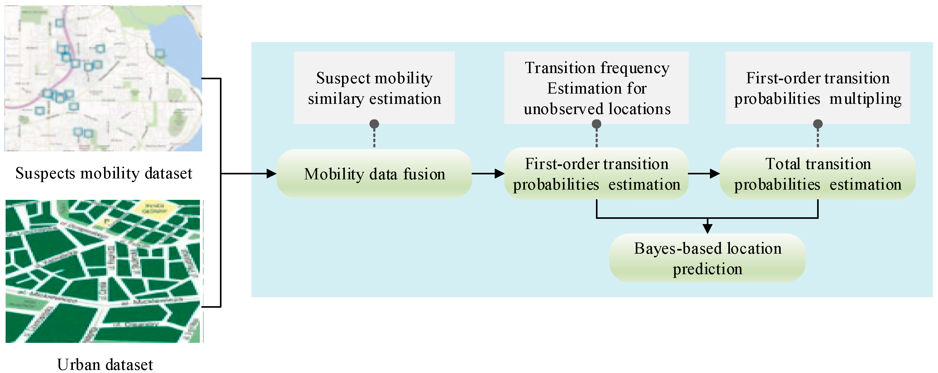
As shown in Figure 1, the prediction process consists of four major parts:

Mobility data fusing: The suspects with a similar mobility pattern to the target suspect are selected. Then, their mobility data are collected as the one of the target suspects.

First-order location transition probabilities estimation: This stage focuses on the transition frequencies estimation for unobserved locations according to the target suspect’s fused mobility data. After that, the transition probabilities in each pair of locations are calculated.

Total location transition probabilities estimation: The total transition probabilities, which are used to model the transition pattern of all possible paths in each pair of locations [34], is indispensable for the multi-step location prediction. The total transition probabilities are obtained by multiplying first-order location transition probabilities.

Bayes-based location prediction: By integrating the first-order location transition probabilities and total location transition probabilities into a Bayes formula, the multi-step location prediction for the target suspect is realized.

3.2. Formal Statement of Problem

Our study aims to predict destinations for the individual suspect using historical trajectories from the suspect’s mobility data. This location prediction problem can be formally expressed as:

Given:

(1) Location set: G = {g₁, g₂,…,g_|G|}, g_i denotes a location (region);

(2) Query trajectory: T^p = {n₁ = g_k+1, n₂ = g_k+2,…, n_j-1 = g_k+t}, n_i denotes a trajectory point, $k,\left(k+t\right)\in \left[1,\left|G\right|\right]$;

Solve: Obtaining the probability of the next point n_j of T^p being g_d:

$$P(n_j=g_d|T^p)$$

(1)

3.3. Basic Concepts and Definitions

Definition 1

(Trajectory location). The observed location that one or more than one mobility points fall in.

Definition 2

(Peripheral location). The unobserved location near a trajectory location without any mobility point falling in.

Definition 3

(Semantic Vector). The semantic vector is: s_r = <s_r1, s_r2, …>, where s_ri is the ith social environment feature of the location r, including crime rate, population, house density, occupation, road density and POI categories, etc.

Definition 4

(Density function). Given a d-dimension space F^d, points p_x and p_y ∈ F^d, the density function that represent the influence of p_y to p_x can be determined by the product of the attribute value c_y in p_y and the kernel function $K(\cdot )$:

$$f_B^y\left(p_x\right)=c_y\times K\left(p_x,p_y\right)$$

(2)

where B represents the kernel function type.

Definition 5

(Density attracting set and Density attracting point). Given the spatial distance function $d(\cdot )$, p_i and p_x ∈ F^d, if {$\exists$p_i| p_i ∈ D, d(p_x,p_i) ≤ ε}, we call D the density attracting set of p_x and call p_i the density attracting point that is attracted by p_x.

Definition 6

(Density value). Given p_x∈ F^d, the density attracting set D = {p₁, p₂, …, p_N} ∈ F^d of p_x, the density value of p_x is the average of the aggregating density function values of all the density attracting points in D:

$$f_B^D\left(p_x\right)=\frac{{\sum }_{i=0}^N{f}_B^i\left(p_x\right)}{N}$$

(3)

Definition 7

(Transition). Given p_x and p_y∈ F^d, p_x is the start point and p_y is the end point, we denote the movement from p_x to p_y as a transition.

3.4. Suspects Mobility Data Fusion

This part aims to estimate the movement similarities between suspects, thereby enabling the model to overcome the data sparsity problem and represent a rich social movement characteristic for the target suspect, by exploring the trajectory data of similar suspects. Two essential steps are:

(1)

Mobility Points Clustering: To make movement patterns of different suspects comparable according to the sparse individual mobility data, we cluster the mobility points of the entire dataset into multiple regions based on spatial semantics similarity and spatial proximity.

(2)

Top-n Similar Suspects: The similarity scores between suspects are measured by overlaps among the spatiotemporal distributions of the regions created in step (1). Therefore, we can easily find the top-n similar suspects of the target suspect by ranking the similarity scores.

The spatial semantics similarity used in step (1) is able to convey social behavior similarity between suspects. Moreover, this rank method gains the advantage of a self-adaption spatial scale for movement similarity calculation.

3.4.1. Mobility Points Clustering

The spatial semantic distance between two trajectory points i and j can be represented by the Cosine applied on their semantic vector s_i and s_j:

$${\rho }_{ij}=cosin\left(s_i,s_j\right)$$

(4)

The unified distance ${\omega }_{ij}$ between i and j is determined by

$${\omega }_{ij}=\{\begin{array}{c}{d}_{ij}\times (1-{\rho }_{ij}), d_{ij}\le \delta \\ \infty , d_{ij}>\delta \end{array}$$

(5)

where $d_{ij}$ is the spatial distance between i and j. δ controls the maximum distance that, if $d_{ij}$ $>$ δ, the points i and j will never be clustered together.

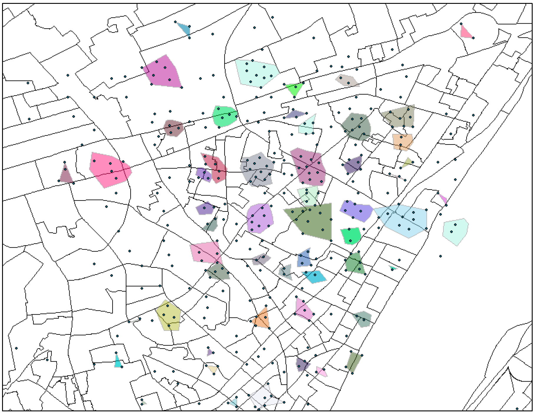
With Formula (5), all of the trajectory points are clustered into different regions using the DBSCAN [55] clustering algorithm. Figure 2 exhibits the regions in a local area, where each colored cluster and/or overlapping points (seen as a single point) denote a region.

3.4.2. Top-n Similar Suspects

The similarity between a pair of suspects is calculated by their temporal visiting distribution of all regions in terms semantic times. Temporal semantics are designed according to the social routine and are classify as the following three-fold.

(1)

Hour bins of day, HBOD ∈ {< 0–6>, < 7–12>, <12–19>, < 20–24>}, denoting before-dawn, morning, afternoon and night, respectively.

(2)

Day of week, DOW = {1 ,..., 7}, representing Monday to Sunday, respectively.

(3)

Rest of Day, ROD = {0, 1}, where 0 express the current day is a rest day, and 1 is a working day.

Intuitively, if location b is visited many times by suspect u, then b must be important for suspect u. Furthermore, a location b that is visited rarely by others will be more representative for suspect u than other common locations. Thus, combining these two ideas, we design the region visiting vector by visiting intensity as follows.

t_u= ≤ q_t,u,1,q_t,u,2,…, q_t,u,s …, >

(6)

where q_t,u,s is the visiting intensity of region s for suspect u in a semantic time t as,

$$q_{t,u,s}=c_{t,u,s}\times \log \frac{\left|U\right|}{I_t\left\{s\right\}}, c_{t,u,s}=\frac{b_{t,u,s}}{b_{t,u}}$$

(7)

where b_t,u is the total visiting number of all the regions at semantic time t for suspect u, b_t,u,s stands for the visiting number of region s at semantic time t for suspect u, and I_t{s} represents the number of suspects that visit the region s at semantic time t.

Relying on $q_{t,u,s}$, the region visiting multinomial distribution of semantic time t for suspect u is defined as:

$$z_{t,u}~multi\left(z_{t,u,1}, z_{t,u,2},\dots ,z_{t,u,\left|S\right|}\right),z_{t,u,i}=\frac{q_{t,u,i}}{{\sum }_j{q}_{t,u,j}}$$

(8)

Then, we use the Jensen-Shannon formula to convey the diversity of the region visiting multinomial distribution between suspects u and v.

$$\mathrm{JSD}\left(z_{t,u},z_{t,v}\right)=\frac{KL(z_{t,u}|\left|l\right)+KL(z_{t,v}||l)}{2}, l=\frac{z_{t,u}+z_{t,v}}{2}$$

(9)

where KL(.) denotes Kullback-Leibler Divergence.

The similarity score between suspects u and v can be defined according to the diversities in all of semantic time T:

$$\mathsf{\Delta }{Q}_{u,v}={\left[{\displaystyle \sum }_{t\in T}\mathrm{JSD}\left(z_{t,u},z_{t,v}\right)\right]}^{-1}$$

(10)

Consequently, by Formula (10), we are able to choose the top-n most similar suspects for the target suspect.

3.5. First-Order Transition Probabilities Estimation

Fusing the trajectory data of similar suspects is an applicable way to alleviate the data sparsity problem. However, these trajectory data are usually insufficient since the visiting information among a number of unobserved locations is unknown. 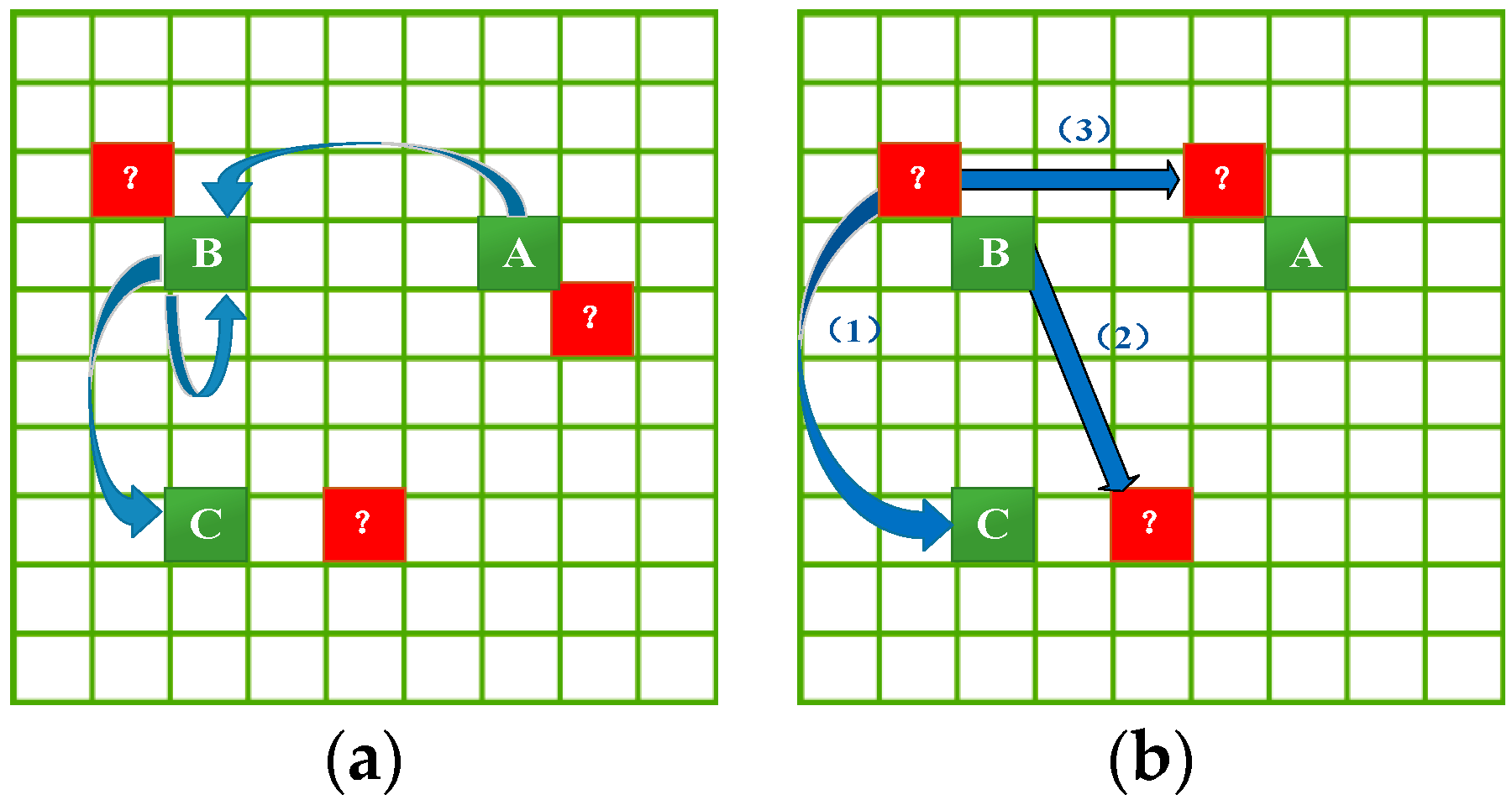As a consequence, the prediction model will fail to unveil comprehensive mobility patterns among more locations, cause the model to suffer from the overfitting problem [53], and further make it incapable of meeting the prediction requirement when the query trajectory contains the unobserved locations. For example, as shown in Figure 3a, given that we already know the transition frequencies (blue arrows) among trajectory locations A, B and C (green grids), we can make a prediction for the query trajectory consisting of any of them. However, we are unable to make a prediction for any query trajectory consisting of the unobserved (peripheral) location (red grids with “?”) because there is no transition information for these locations in the mobility dataset.

Therefore, to improve the generalization capability of the prediction model, this section will estimate the transition frequencies in three instances as shown in Figure 3b: (1) transition frequencies from peripheral locations to trajectory locations; (2) transition frequencies from trajectory locations to peripheral locations; and (3) transition frequencies from peripheral locations to peripheral locations. These transition frequency estimations follow the principles below.

(1)

A significant characteristic of human activity is that the transition probability from one location to another one is inversely proportional to the distance between them [46]. Therefore, we can exploit such a geographical characteristic to build the transition patterns for an unobserved location from its spatially adjacent observed locations.

(2)

The similarity in social environment between locations that are nearby each other may lead to similar crime spatial activity patterns and transition patterns for them [56,57]. Thus, it can be leveraged such spatial semantic similarity to help us estimate the transition probabilities for unobserved locations.

The challenge is how to quantify and utilize the influences of both spatial adjacency and spatial semantics to estimate the transition frequencies for peripheral locations. This research addressed the challenge via a KDE-based smoothing technique. To the best of our knowledge, this is the first attempt to infer the transition patterns for unobserved locations by jointly exploring geographical influence and spatial semantics. In the following, we elaborate this procedure.

3.5.1. Transition Frequencies from Trajectory Location to Peripheral Location

We assume that p_x is the peripheral location, that the trajectory location p₀ is the starting point of N transitions Ʈ = {${𝓉}_1,\dots , {𝓉}_N$}, and that D = { p₁, p₂, …, p_N } is the density attracting set of p_x. The trajectory locations p₁, p₂, …, p_N are the end points of transitions in Ʈ. Given the transition frequency $c_i^0$ from p₀ to every p_i ∈ D, the transition frequency from p₀ to p_x can be obtained by aggregating $c_i^0$ and dividing it by N according to Formula (3) when only considering the spatial proximity:

$${\acute{c}}_x^0=f_{gauss}^D{\left(p_x\right)}_d=\frac{{{\displaystyle \sum }}_{i=0}^N{f}_{gauss}^i\left(p_x\right)}{N}=\frac{\frac{1}{2\pi h_d}{{\displaystyle \sum }}_{i=1}^N{c}_i^0\times exp{\left[-\frac{d\left(p_x,p_i\right)}{2h_d}\right]}^2}{N}$$

(11)

where gauss means that we use a Gaussian kernel function, d(p_x,p_i) indicates the spatial distance between p_x and p_y, and h_d is the bandwidth for spatial distance in the kernel function.

If we only consider the spatial semantics closeness, the above Formula (11) transforms to:

$${\stackrel{`}{c}}_x^0=f_{guass}^D{\left(p_x\right)}_s=\frac{\frac{1}{2\pi h_{s}N}{{\displaystyle \sum }}_{i=1}^N{c}_i^0\times exp{\left[-\frac{consin\left(s_x,s_i\right)}{2h_s}\right]}^2}{N}$$

(12)

where h_s is the bandwidth for spatial semantics closeness in the kernel function.

When both spatial distance and semantics closeness are considered simultaneously, we will obtain the unified transition frequency by combining Formulas (11) and (12)):

$$c_x^0=a_1{\acute{c}}_x^0+\left(1-a_1\right){\stackrel{`}{c}}_x^0$$

(13)

where a₁ $\in \left[0,1\right]$ is a weight controlling the influences of spatial proximity and spatial semantics on the transition frequency.

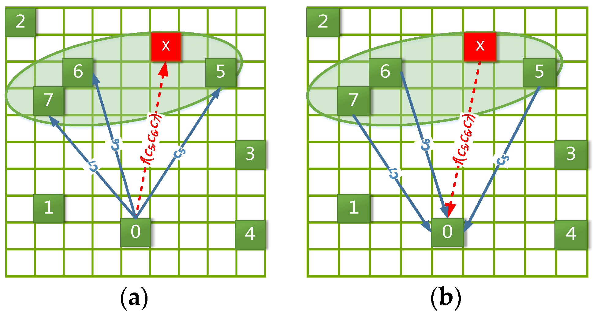
For example, as shown in Figure 4a, p_x is a peripheral location (red grid), and its density attracting set D is composed of the trajectory locations p₅, p₆ and p₇ (green grids located in the green eclipse). Meanwhile, c₅, c₆ and c₇ (blue arrows) denote the known transition frequencies from p₀ to p₅, p₆ and p₇, respectively. Then, we can estimate the unknown transition frequency (red dotted arrow) from p₀ to p_x by importing c₅, c₆ and c₇ into Formulas (11)–(13).

3.5.2. Transition Frequencies from Peripheral Location to Trajectory Location

By the same process mentioned above, we are able to estimate the transition frequency from a peripheral location to a trajectory location. Formally, assume that the trajectory location p₀ is the end point of N transitions Ʈ = {${𝓉}_1,\dots , {𝓉}_N$}, D = { p₁, p₂, …, p_N } is the density attracting set of the peripheral location p_x, and the trajectory locations in D are the starting points of the transitions in Ʈ. Given the transition frequency $c_0^i$ from p_i ∈ D to p₀ in each transition of Ʈ, the transition frequencies from p_x to p₀ can be obtained by Formulas (11) and (12) as ${\acute{c}}_0^x$ and ${\stackrel{`}{c}}_0^x$, respectively. Therefore, the final transition frequencies from p_x to p₀ are

$$c_0^x=a_2{\acute{c}}_0^x+\left(1-a_2\right){\stackrel{`}{c}}_0^x$$

(14)

where a₂ $\in \left[0,1\right]$ is a weight.

The corresponding example plot is shown in Figure 4b with almost the same processing as in Figure 4a. Its description is omitted to avoid repetition.

3.5.3. Transition Frequencies from Peripheral Location to Peripheral Location

We learn of the transition frequency from peripheral location p_x to another peripheral location p_y through two aspects: (1) deeming p_y as the trajectory location as in Section 3.5.2 and (2) regarding p_x as the trajectory location as in Section 3.5.3. Then, we combined the two estimated visiting frequencies, denoted as c_xy and c_yx, respectively, to produce the final result $c_y^x$:

$$c_y^x=a_3{c}_{xy}+\left(1-a_3\right)c_{yx}$$

(15)

where a₃$\in \left[0,1\right]$ is a weight.

It should be noted that only by estimating all the transition frequencies between peripheral locations and trajectory locations can we obtain the transition frequencies between peripheral locations.

3.5.4. Markov Location Transition Matrix

Thus far, we are able to compute the first-order transition probabilities, which are utilized to build the Markov transition matrix M:

$$M=\left[\begin{array}{ccc}{p}_{00}& \dots & p_{0G}\\ \dots & p_{ij}& \dots \\ p_{G0}& \dots & p_{GG}\end{array}\right],p_{ij}=\frac{c_j^i}{{\sum }_{k\in G}{c}_k^i}$$

(16)

where G denotes all of the locations.

3.6. Total Transition Probability Estimation

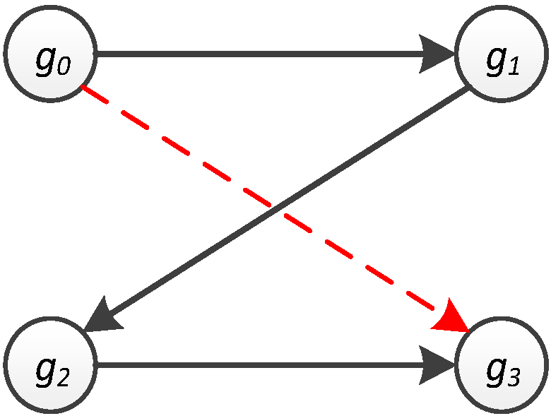
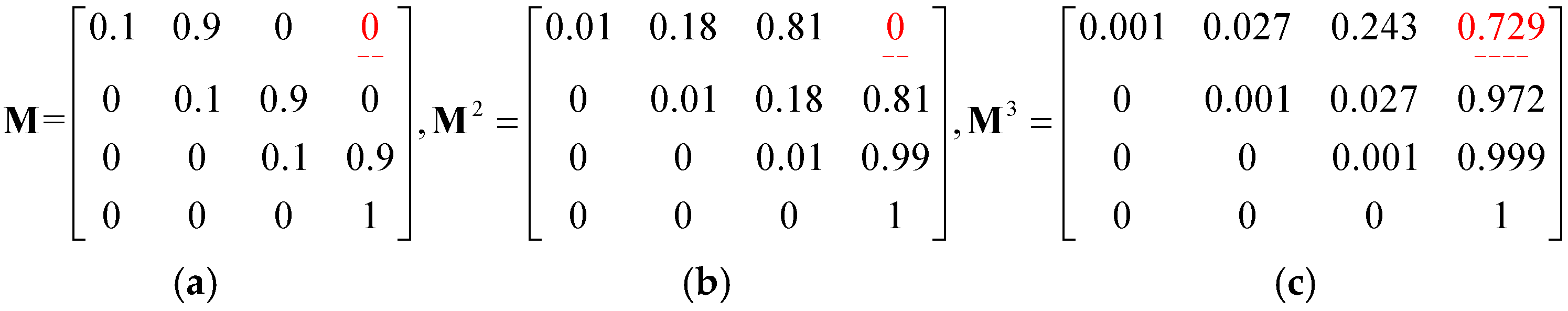
Next, we need to calculate the total transition probability p_i→j that expresses the transition probability between a pair of locations through all possible paths, each of which is made up of a number of bypass locations. Luckily, this total transition probability can be generated from M by multiplying itself. In general, M^1+r (r ∈ [0, ∞)) holds the probabilities of transition from one location to another one in exactly r steps (bypass locations). The following example demonstrates the concept of the total transition probability. By referring to Figure 5 and Figure 6a, the probability of travelling from g₀ to g₃ is found to be zero (${\mathrm{M}}_{03}^1$ = 0) because M only stores the probability of movement from one location to another through exactly zero steps (bypass locations). Nevertheless, when M is multiplied by itself 2 times to form M₃, each entry in it indicates the transition probability from one location to another in two steps. Hence, the transition probability from g₀ to g₃ through 2 steps is 0.729 (${\mathrm{M}}_{03}^3=0.729$), as shown in Figure 6c.

According to the multi-step products of M, we can obtain the total transition probability p_i→j by the sum of r-step transition probabilities of all possible paths between p_i and p_j. Formally [34]:

$${\mathrm{p}}_{i\to j}={\displaystyle \sum }_r{M}_{ij}^{r+1}$$

(17)

However, two problems also arise:

(1)

The paths with different numbers of steps do not necessarily have the same influences on the total transition probability. For instance, the pair of locations with short spatial distance prefers a small number of steps rather than many bypass locations. Therefore, how are we to capture various influences of different M^r on the total transition probability?

(2)

How do we define the maximum value of r since the number of paths from one location to another is infinitely large without restrictions?

For the first question, people including suspects usually travel in a short path to make the cost (e.g., time, expense or energy) as small as possible even though a detour distance may be taken sometimes. Therefore, the shortest path generally makes the greatest contribution to the total transition probability, and the path with more bypass locations makes a lesser contribution to the total transition probability. Thus, we can give different weights to different r-step transition probabilities and sum them up as the total transition probability ${\tilde{p}}_{i\to j}$, formally,

$${\tilde{p}}_{i\to j}={{\displaystyle \sum }}_{r\to r_{max}}{w}_r{M}_{ij}^{r+1}{w}_r=\frac{k_r}{{\displaystyle {\sum }_j{k}_j}},k_r=f(r)=\exp (-\frac{r}{d_{ij}})$$

(18)

where d_ij is the spatial distance between locations i and j. When d_ij is fixed, a large r will cause a small w_r, reflecting the fact that a path with too many bypass locations is seldom chosen by suspects.

For the second question, the existing study of [34] gives the answer that the maximum step r_max is usually 1.2 times the shortest steps between the start and end locations. However, this idea only fits specific trajectory datasets. Furthermore, it may yield an irrelevant r_max when focusing on a different individual suspect. It is suggested that r_max should account for the shortest steps of the target suspect as well as the spatial distance between the two locations. The procedure to compute the r_max for an individual suspect is shown as below.

(1)

Give a constant value q > 1, assuming it equals to 2.

(2)

Build a transition weight matrix H. If there is no transition between locations g_i and g_j, the entry H_ij = ∞; if the target suspect is involved in this transition, H_ij = 1; else, H_ij = q.

(3)

Obtain the top-k shortest paths [56] based on H in which the entries are considered to be the distances among locations;

(4)

Computer the conformity t_m for every path m in the top-k shortest paths by

$$t_m=\frac{a_4{e}_m+(1-a_4)l_m}{r_m}$$

(19)

where a₄ is a fixed coefficient larger than zero, l_m denotes the distance of path m, r_m denotes the number of bypass locations in path m, and e_m denotes the number of locations visited by the target suspect in path m. Therefore, a path with more locations that the target suspect has visited and fewer bypass locations has more power to describe the r that the target suspect prefers.

The number of bypass locations r_max in the path with the largest conformity t_max is what we need.

Once w_r and r_max are obtained, we can efficiently compute the total transition probability matrix for all pairs of locations by a dynamic programming method [34].

3.7. Bayes-Based Location Prediction

The probability of a location $g_d$ being the destination can be computed as the probability that n_j contains the destination location $g_d$ conditioning on the query trajectory T^p. This probability was previously given in Formula (1) and is extended using Bayer’s inference here as:

$$P\left(n_j=g_d|T^p\right)=\frac{P(T^p|n_j=g_d)\times P\left(n_j=g_d\right)}{{{\displaystyle \sum }}_{k=1}^{g\times g}P(T^p|n_j=g_k)\times P\left(n_j=g_k\right)}$$

(20)

The prior probability $P\left(n_j=g_d\right)$ is easily obtained through

$$P\left(n_j=g_d\right)=\frac{\left|D_d\right|}{\left|D\right|}$$

(21)

where $\left|D_d\right|$ is the visiting times of $g_d$ and $\left|D\right|$ is the visiting times of all locations.

The posterior probability $P(T^p|n_j=g_k)$ is calculated as [34],

$$P\left(T^p|n_j=g_d\right)=\frac{P\left(T^p\right)\times p_{\left(j-1\right)\to j}}{p_{1\to j}}$$

(22)

where P(T^p) is the path probability of the query trajectory T^p; p_(j-1)→j is the total transition probability of moving from n_(j-1), the end location of T^p, to the predicted destination n_j = $g_d$; and p_1→j is the total transition probability of travelling from n₁, the starting location of T^p, to n_j = $g_d$.

The path probability P(T^p) can be obtained by:

$$P\left(T^p\right)={{\displaystyle \prod }}_{k=1}^{j-1}{p}_{k\left(k+1\right)}$$

(23)

where p_k(k+1) is the first-order transition probability between locations n_k and n_(k+1).

Now, the first-order transition probabilities coming from Formula (16) and the total transition probabilities coming from Formula (17) can be inserted into Formulas (23) and (22), respectively, to fulfill the location prediction task. The complete location prediction algorithm is shown in Algorithm 1.

Algorithm 1. Location Prediction Algorithm.

Input: query trajectory Tp = {n1,…,n(j−1)}

Output: top-k predicted locations.

1 list = ∅;

2 construct path probability P(Tp) from M;

3 Foreach nj in G do

4  Retrieve p1→j and p(j-1)→j from Mr;

5  Compute $P\left(n_j=g_d\right)$;

6  Compute P(Tp | nj = $g_d$);

7  Compute P(nj = $g_d$ | Tp);

8  Store P(nj = $g_d$ | Tp) in list;

9 sort list;

10 return: top-k elements in list.

4. Experimental Section

In this section, we conduct an extensive experimental study to evaluate the performance of our CMoB.

4.1. Data Preparation

4.1.1. Study Area

Wuhan is the capital of Hubei province and is one of the largest cities in central China. It lies in the eastern Jianghan Plain at the intersection of the middle reaches of the Yangtze and Han rivers. The city of Wuhan has a population of 10,766,200 people as of 2016, and its urban administration consists of 7 central districts (Qiaokou, Jianhan, Jiangan, Hanyang, Wuchang, Hongshan, and Qiangshan) and 6 suburban and rural districts (Dongxihu, Hannan, Caidian, Jiangxia, Huangpi and Xinzhou).

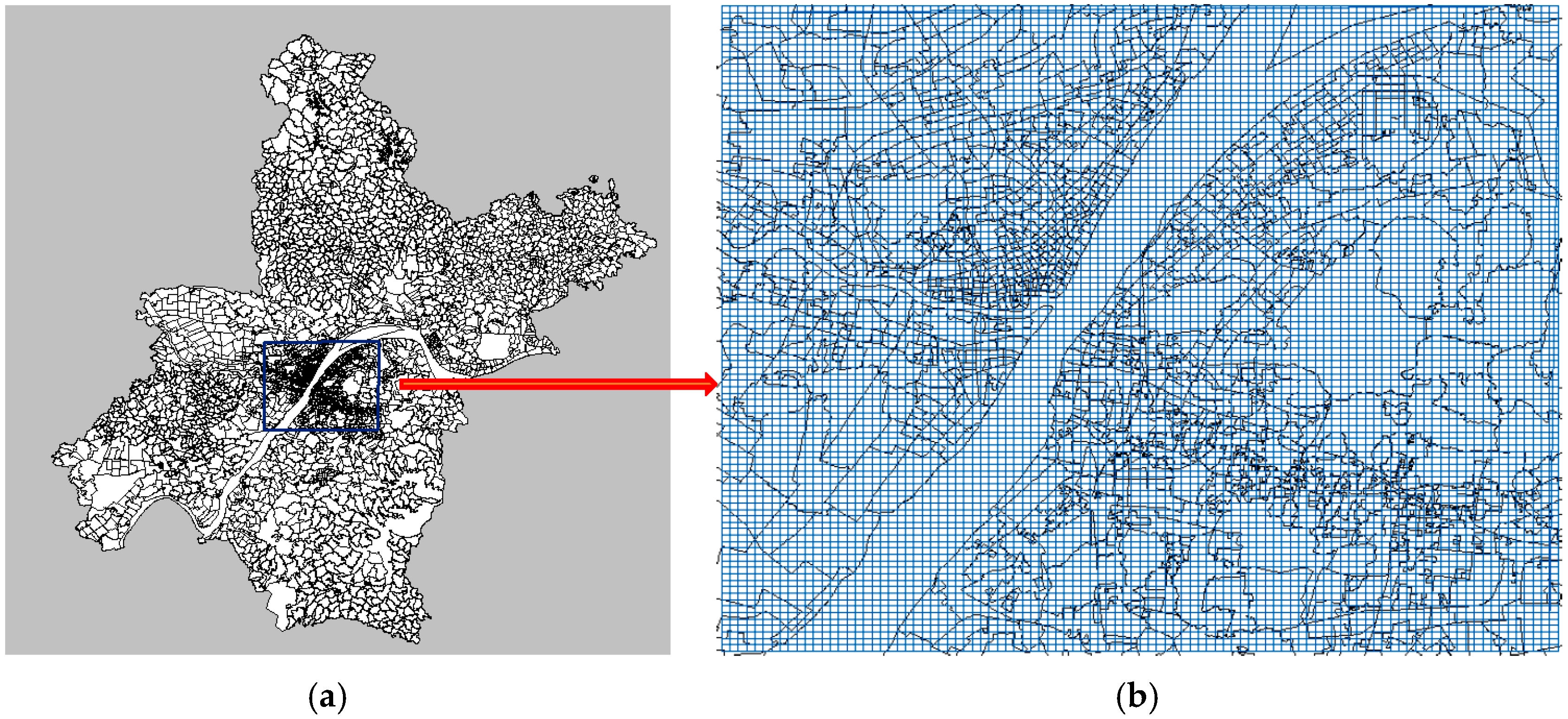
This paper built 100 × 100 grids to cover the 570-km² urban areas of Wuhan City as shown in Figure 7, and each of grid (256 m × 224 m) denotes a location as the basic spatial unit.

4.1.2. Data Sources

Four types of datasets are used to test the location predictions, including a suspect mobility dataset, criminal dataset, POI dataset, and demographic dataset. The detailed information of each dataset is described below.

(1) Suspect Mobility Dataset

This dataset, which was reported to the Wuhan Police Department, includes 18,754 records of 210 suspects within 6 months (January–June 2012) in Wuhan city, distributed across 1083 different venues. A trajectory can be represented as the sequence of grids that cover the locations of a suspect recorded in the dataset according to the temporal order in one day. There are 10,537 trajectories in total. A large number of locations in the records are described as text addresses, such as "Yinxing Drifting Wood shop, No. 557 Liberty Avenue Wuhan City", “Changxin Digital Hongyuan Shop the 1st floor Ya’an Garden, science museum road” etc. Therefore, we converted these text addresses into longitudes and latitudes by Geocoding web services from Baidu [57] and Geopy [58]. It should be noted that the geocoding web services will randomly introduce artificial errors. However, by checking some results of geocoding services with real coordinates, we found that these artificial errors are so small that they will not lead to a venue transfer from one grid to another grid, which means that these artificial errors will not influence the effects of our model and baseline methods.

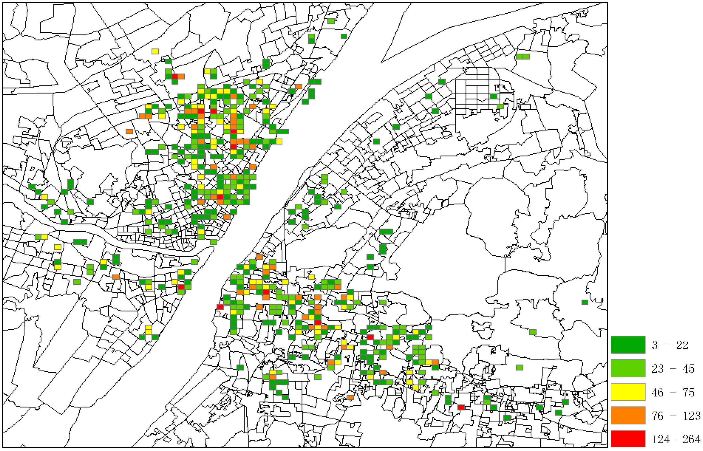
After data cleaning processing, 65 records were filtered out because their text addresses were unresolvable in geocoding web services, and together with records referring to suspects who have fewer than 10 records in dataset. At last, 179 suspects with 17,516 records (containing 1050 venues and 10,195 trajectories) are left as the final dataset. The spatial distribution of suspects is shown in Figure 8, where the colors in grids denote the different accessing intensities by all suspects.

There are several characteristics about the final dataset:

• The mobility data for each suspect is extremely sparse. For example, there are 70% of suspects with fewer than 50 records, 83% of suspects with fewer than 50 trajectories, and 80% of them with fewer than 8 different venues. It can also be inferred that each suspect was frequently detected in several limited areas.
• The distances between continuous trajectory points varied from 0 km to 10 km.
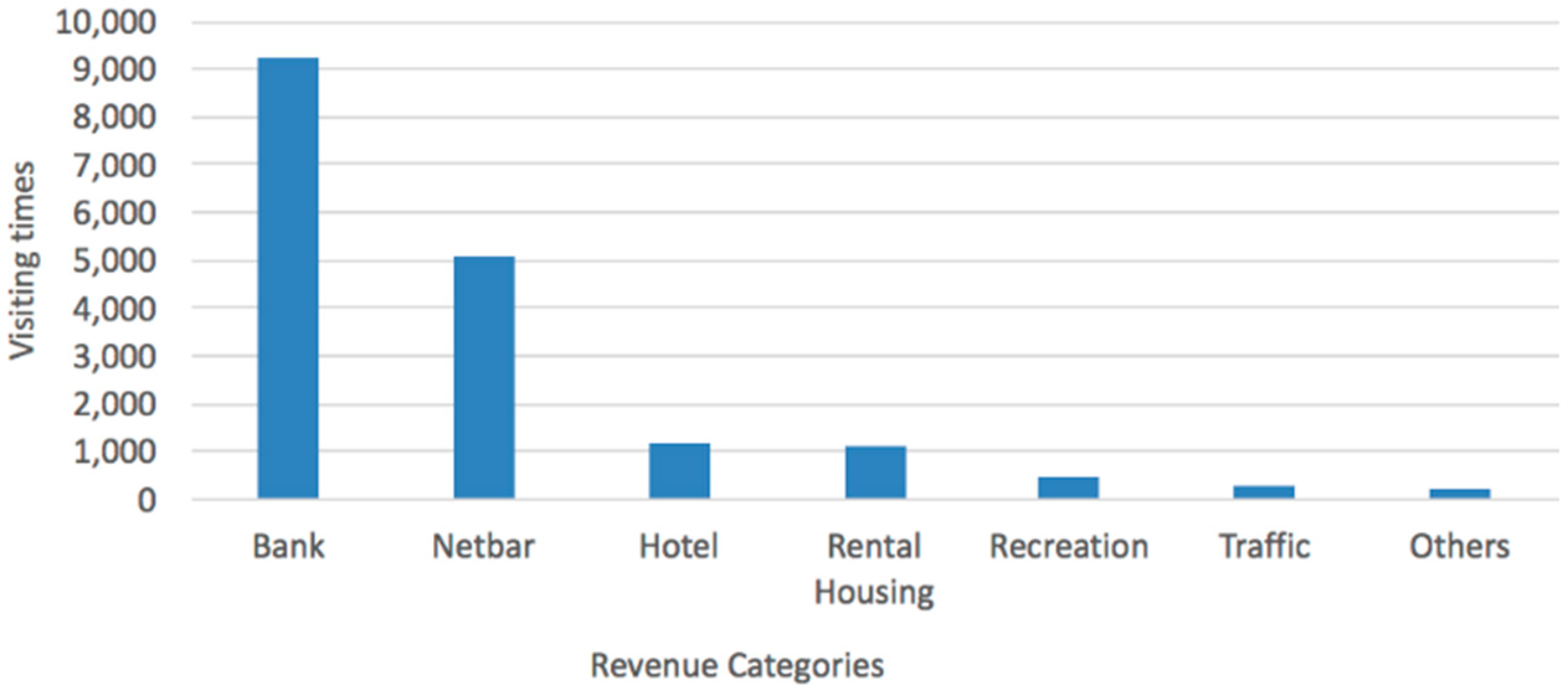
• The visiting distribution of venue types is shown in Figure 9, where the suspects accessed banks (mostly ATM machines) up to 9207 times. The second highest accessing place is cybercafés, followed by hotels, rental housing, recreation, traffic sites (airports and bus stations, etc.) and other types (such as shopping malls, etc.).

(2) Criminal Dataset: It includes 105,347 criminal incidents of Wuhan city from January–December 2012, with the offense type and coordinates for each incident.

(3) POI Dataset: This dataset consists of 102,641 POIs in 12 categories, containing restaurant, traffic station, hotel, residential community, education, entertainment, shop, government, factory, company, hospital and bank.

Demographic dataset: There are 3602 communities with demographic information for each community. The demographic information contains population, education, sex, birth date, nationality and occupation. The datasets from (2) to (4) are all obtained from the Wuhan Police Department and are utilized as the spatial semantics to find similar suspects (in Section 3.4.1) and estimate transition frequencies for the unobserved locations (in Section 3.5.1, Section 3.5.2 and Section 3.5.3).

4.2. Evaluation Metrics

We use three metrics to measure the performance of location prediction models:

(1)

Top-k Precision [54] (TP): If the correct destination falls within the top-k predicted locations, this time is considered to be the correct time. Thus, the ratio of correct times to the total times is called top-k precision. The higher this metric value is, the better performance the model has.

(2)

Top-k Error (TE): The shortest distance between the top-k predicted locations and the correct destination. If k = 1, it is called Accuracy Measures [27]. This metric is used to indicate how far the prediction results deviate from the true destinations. A better algorithm has a lower distance deviation.

(3)

Missing Percentiles (MP): The percentage of occurrences for which a model cannot give any result. This metric is used to evaluate the impact of the data sparsity on the robustness of the models. A better algorithm has a lower missing percentile.

k in the metrics of (1) and (2) specifies the number of locations (grids) that have to be searched to identify the correct destination. A large k relates to more locations needing to be searched by police forces, as well as more resources needing to be consumed. Therefore, k should be adjusted according to the compromise between consumable resources and preferable metric performance in the actual application. If it is not specified, we define k = 9.

In this work, we define the distance of the two grids as the distance between their centers.

4.3. Baselines

In experiments, we randomly chose ten suspects with m similar suspects for each of them. Hence, we carried out eleven experiments to evaluate the performance for each model as m increases from 0 to 20.

As discussed in Section 1, no related work has been proposed to the multi-order location prediction for individual suspects based on the query trajectory. However, we use the following LBSN-related methods, which are equivalent to state-of-the-art methods as baselines.

Markov: it employs the first-order location transition matrix to predict the location. Most existing location prediction methods are actually variants of the Markov model. Particularly, [54] employed the Markov model to model the neighbor road selection probabilities for individual offenders, though the probabilities were not used to present the transition patterns between arbitrary distance locations as this paper did. The Markov model therefore represents the general class of location prediction models without dealing with the data sparsity problem.

ZMDB [44]: This method is used for the multi-order location prediction. It first counts the number of trajectories satisfying two conditions: (i) it is partially matched by the query trajectory T^p; (ii) it terminates at a location in n_j. The count is then divided by the number of trajectories that terminate at a location in n_j to serve as the posterior probability. Formally,

$$P(T^p|d=n_j)=\frac{\left|\left\{T_{d=n_j}|T^p\subset T_{d=n_j}\right\}\right|}{\left|T_{d=n_j}\right|}$$

(24)

where $\left|\left\{T_{d=n_j}|T^p\subset T_{d=n_j}\right\}\right|$ denotes the number of trajectories that satisfy both aforementioned conditions and $\left|T_{d=n_j}\right|$ denotes the number of trajectories that terminate at a location n_j. Afterwards, Formula (24) is substituted into Formula (20), thus yielding the probability of n_j as the destination. Compared with Markov, ZMDB holds the advantage of modeling multi-order location transitions.

SubSyn [34]: This approach realizes the multi-order location prediction by decomposing suspects’ trajectories into a Markov matrix and total transition probabilities. However, the difference between it and our approach lies in two aspects: it does not estimate the transition patterns for unobserved locations, and the number of bypass locations when computing the total transition probability is a fixed value. In addition, this model is trained using the trajectory data of all of ten suspects in each experiment to simulate the way of synthesizing the mobility data of all users in [34].

For the proposed CMoB, the gridding-searching method [59] is involved to search for the optimal parameters for the proposed CMoB. To illustrate the step, a numbers of parameter sets were sampled from the space in

Table 1. Parameters spaces.

Parameter	Parameter Space
ε	{300, 350, …, 800}
hd	{100, 200, …, 500}
hs	{0.1, 0.2, …, 0.5}
a1	{0, 0.1, …, 1}
a2,	{0, 0.1, …, 1}
a3	{0, 0.1, …, 1}
a4	{0, 0.1, …, 1}

.

Then, top-k precision was used as a criteria for selecting the optimal parameter sets, which were finally assigned as: ε = 650 m, h_d = 300 m, h_s = 0.1, a₁ = 0.5, a₂ = 0.5, a₃ = 0.5 and a₄ = 0.7.

For all of the models, if any of them fails to find the predicted destination, we use the last point in the query trajectory as the predicted one.

4.4. Results Evaluation of Top-k Error

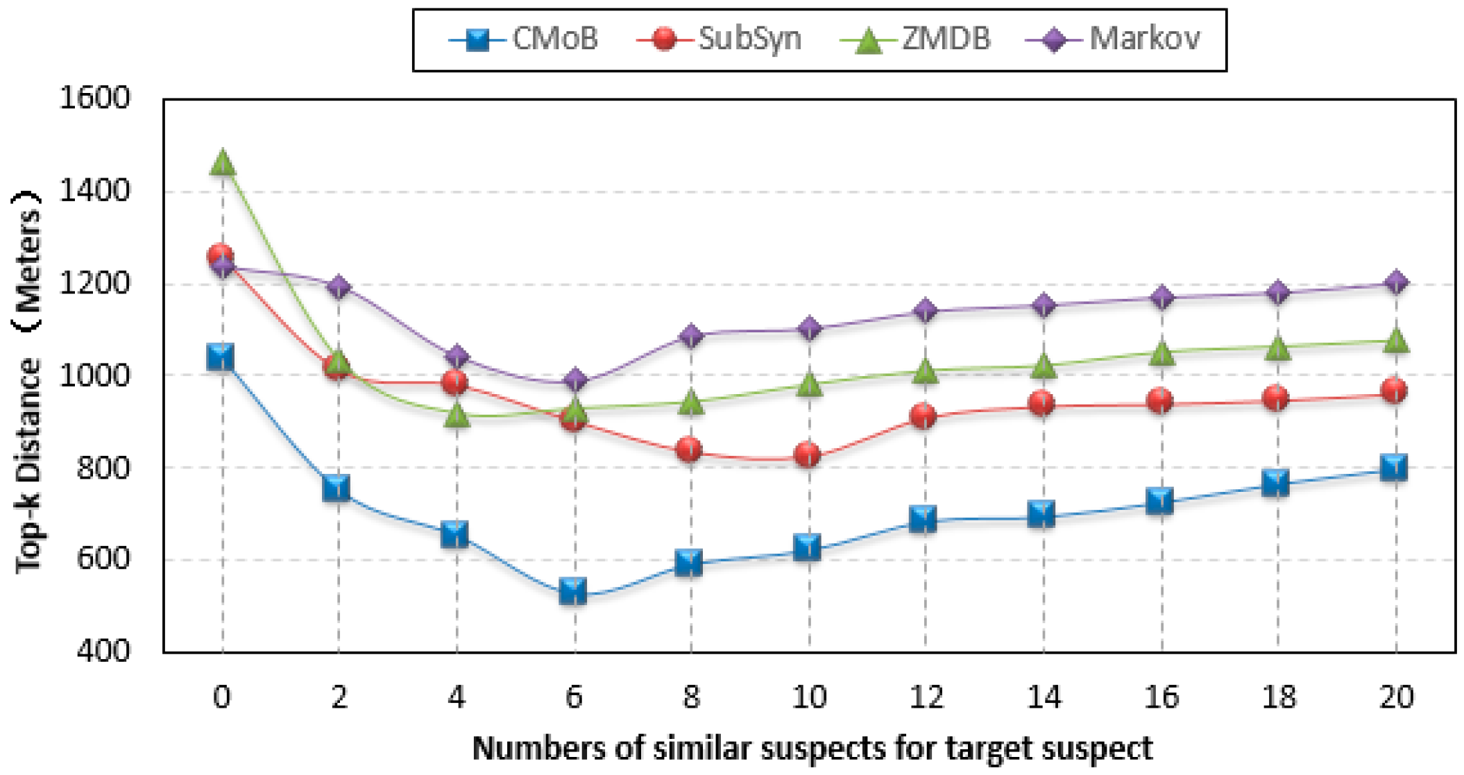
As shown from the curves in Figure 10, the performance of our CMoB on TE (top-k error) is outstanding among the four models. In particular, with the increase of m, the TEs of the other three baseline methods are all higher than 800 m, while that of CMoB is below 800 m most of the time. When m = 0, which means there is no external trajectory data to be leveraged, the TE of CMoB is lower than those of SubSyn, ZMDB and Markov by 20%, 20% and 40%, respectively, yielding a significant improvement in performance, because CMoB is capable of alleviating the data sparsity by the estimation of transition frequency for unobserved locations. As m continues to increase, the TEs of all models decrease since more external trajectory data weaken the data sparsity problem. For instance, when m increases from 0 to 6, the TE of CMoB keeps decreasing, and that of SubSyn keeps decreasing when m increases from 0 to 10. The best TE of each model is also obtained during the processing, where the best TE of our proposed model is 527 m and those of the other three models stay in the 800–1000 m range, which means that the performance of our model is better than the others by approximately 80–100%. However, when the value of m is beyond a certain threshold, the performances of all the models decline owing to the difference of mobility patterns between the target suspect and later employed similar suspects growing wider. For example, when m > 6, the TE of CMoB and Markov start to increase. With m is beyond a certain threshold, the new employed trajectories become geographically far away from those of target suspects, thus posing lower and lower impacts on the transition patterns of the focus areas where the targeted suspect stayed. Therefore, the TEs of all models tends to be a constant value at this stage. For instance, the TEs of CMoB and Markov tend to 800 m and 1200 m, respectively, when m > 6. This situation also suggests that a large value of m (too many similar suspects) will have little influence on the performance of the prediction model. Here, when m increases to 20, the performance of the proposed CMoB still excels compared to the other baseline models by approximately 20–50%.

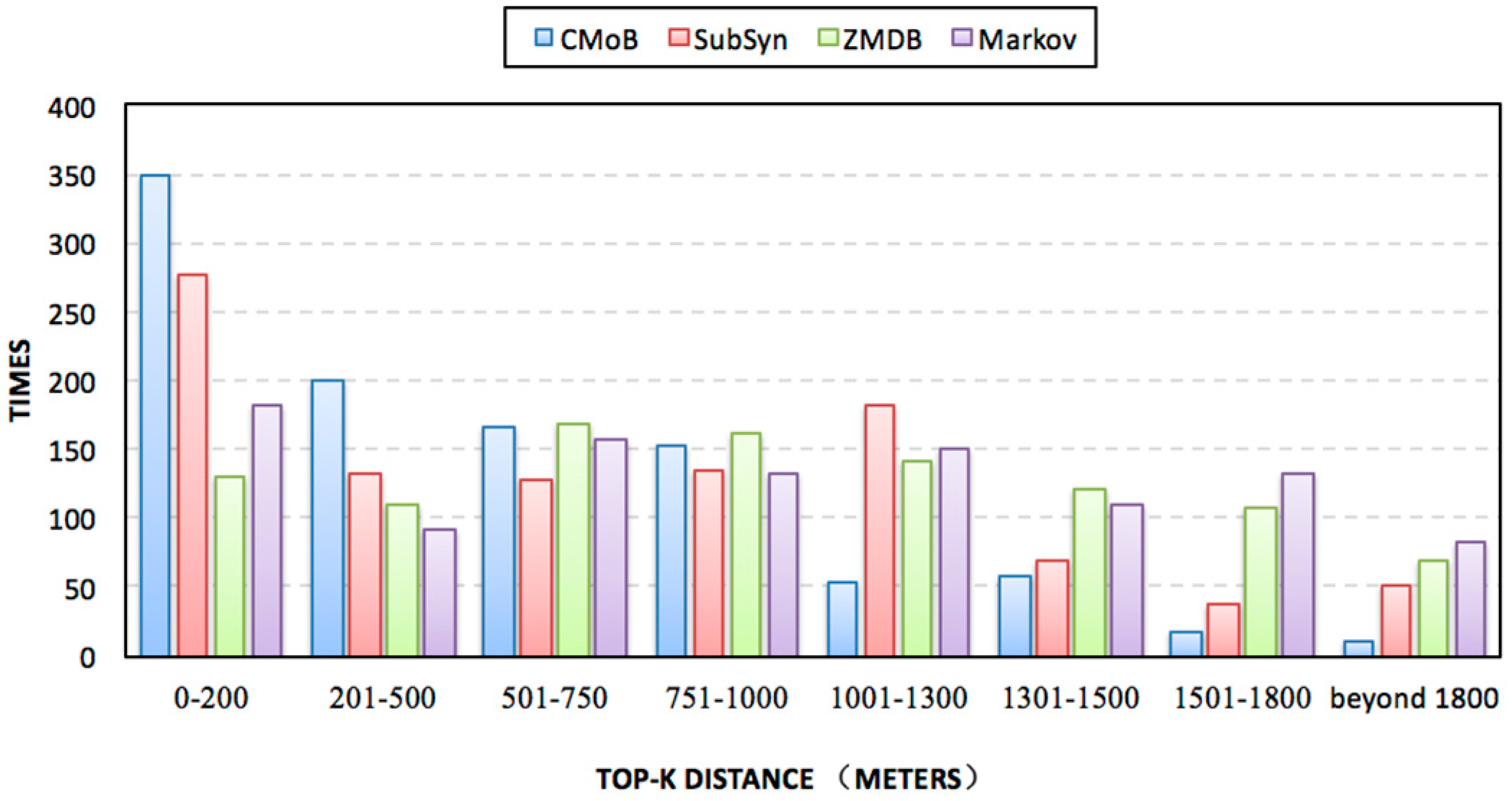
Figure 11 gives the histogram of the occurrences for different TEs during experiments, where the high occurrence at low TE represents excellent performance. From the plot, we can find that the occurrences of CMoB at TE < 500 m accounted for 50% of the total occurrences, showing that most predicted locations of CMoB are close to the correct destinations compared to other baseline methods. As TE increased, the occurrences of CMoB reduced dramatically, with approximately 90% of the total occurrences being concentrated in TE < 1000 m. For SubSyn, the occurrences demonstrate a decreasing tendency as TE increases, and approximately 40% of the occurrences are allocated in TE < 500 m, while approximately 68% are located with TE < 1000 m. For ZMDB and Markov, the discrepancies of occurrences along with different TD are inconspicuous. Their 50% of occurrences remained at TE > 1000 m, implying extremely low performances when they confront the data sparsity problem. Moreover, for Markov, there are 82 occurrences appearing for TE between 750 m and 1800 m, which is the largest value among all models, indicating the worst performance among all models.

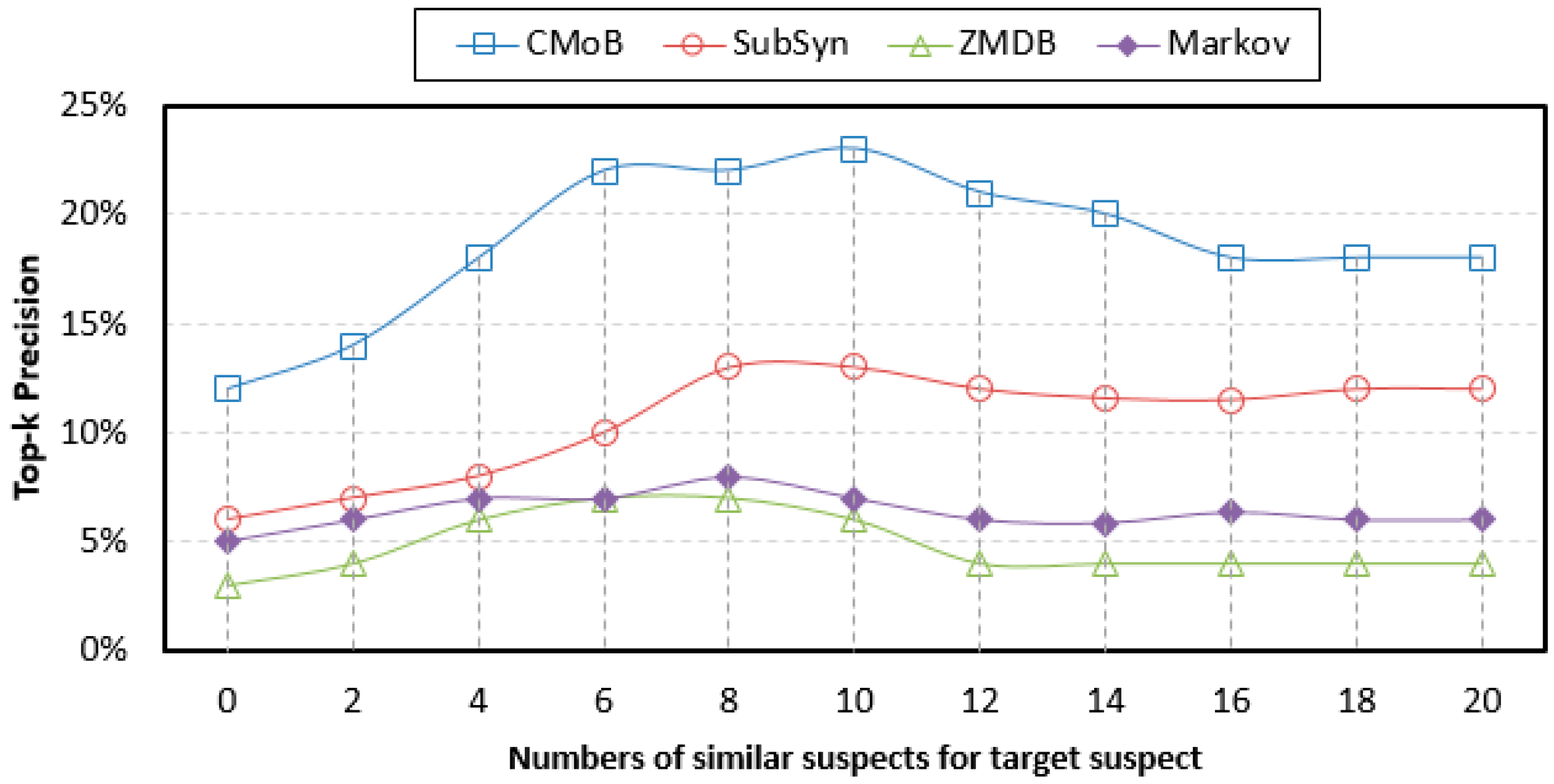
4.5. Evaluation of Top-k Precision

From Figure 12, we can discover that with the growth of m, the TP (top-k precision) of our CMoB are distributed in 12–23%, higher than those of the three baseline methods, in which the performance of ZMDB is the lowest, with its best TP being only 7%. When m = 0, our CMoB achieves 12% on TP, which is higher than those of the others by 100–200%, implying that CMoB has the ability to reveal transition patterns for more locations. With the growth of m, more newly employed mobility data are located in the areas where the target suspect concentrated on so that all prediction models are able to obtain the transition patterns for more locations, resulting in the improvement in their performances on TP. For example, as m increased from 0 to 10, the best TP of CMoB reached 23%, with the improvement rate being beyond 90%, higher than the other three baseline methods by 100–300%. Along with the growth of m, more mobility data of un-similar suspects are introduced, which makes TPs of the four models gradually decline to some fixed values, according to the same reason explained in Section 4.4, when the performances of TE also declined to fixed values as m increased beyond a certain threshold.

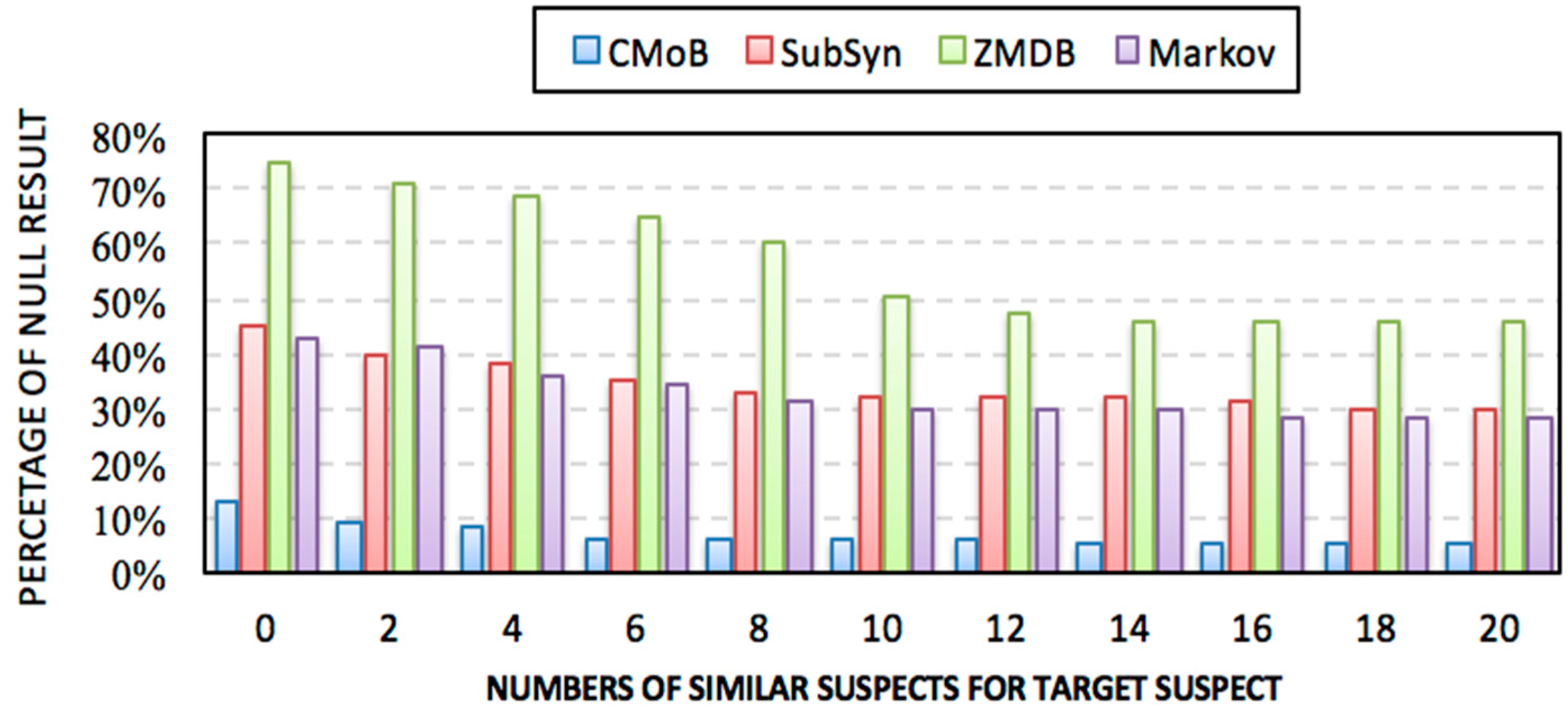
4.6. Evaluation of Missing Percentiles

Figure 13 shows that the missing percentiles (MP) of all models decrease along with the increase of m. Specifically, CMoB achieves the best performance among them with the MP below 10% most of the time. Compared with CMoB, the performance of ZMBD remains the lowest at all times, with its MP up to 45%, while the MPs of SubSyn and Markov are all higher than 30% for the most part. Moreover, for the metric of average MP, CMoB is five times lower than SubSyn, eight times lower than ZMDB and four times lower than Markov, indicating that data sparsity is fatal to the robustness of the model, which lacks appropriate solutions to address the issue.

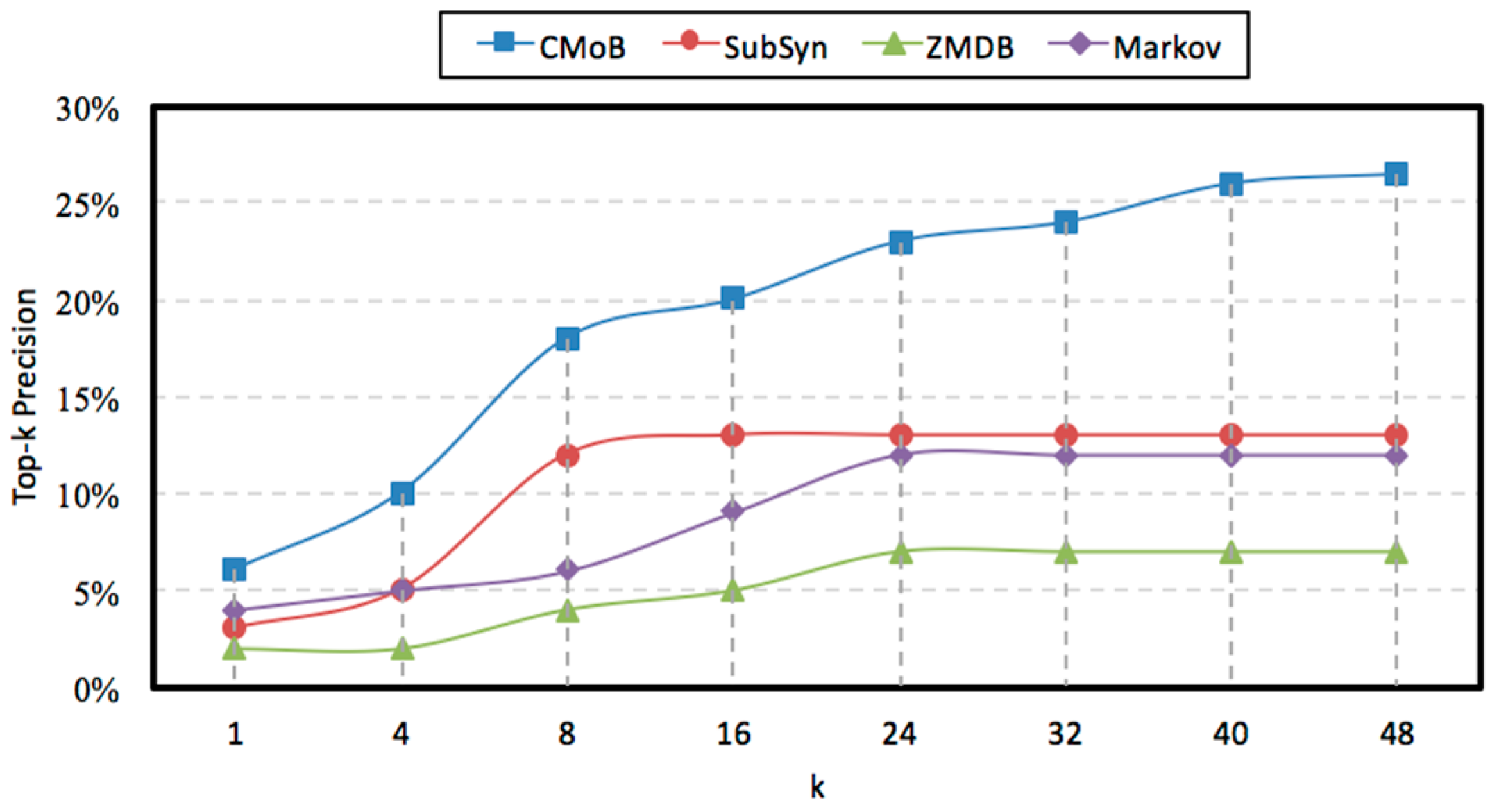
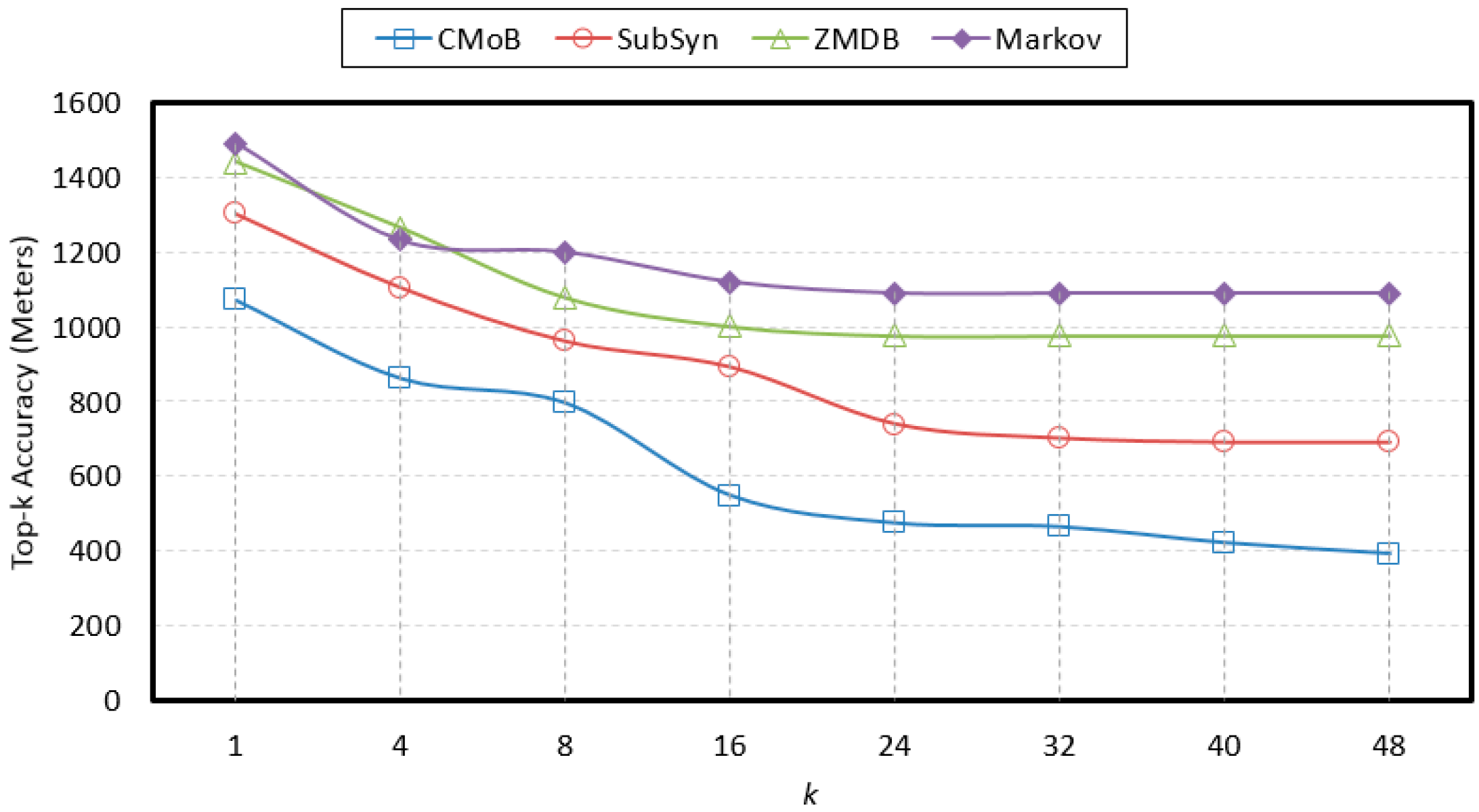
4.7. Evaluation of k

With the rise of k, the variations of prediction performances on TE and TP are shown in Figure 14 and Figure 15 when m = 20. It can be observed that the performances of CMoB are much better than the other 3 baseline methods at any k value. Meanwhile, as k reaches a critical value, the performances of SubSyn, ZMDB and Markov on TP and TE no longer changed. For example, when k > 24, the TE of ZMDB and Markov stopped at 976 m and 1091 m, respectively. Similarly, when k > 24, the TP of Markov and SubSyn no longer change, staying at 14% and 12%, respectively. However, with the increase of k, the performances of CMoB continued improving, where its TE falls down from 1072 m to 392 m and TP increases from 6% to 27%. Moreover, the improvement rates of CMoB on the two metrics are still the largest among these four models. This is because CMoB can obtain the transition patterns for more locations so there were more candidate predicted locations in its results. With the growth of k, the opportunities for observing shorter distances between the correct destination and the top-k candidate locations increase, and the correct destination is more likely to be found in the top-k candidate results. However, for the other three baseline methods, the numbers of candidate predicted locations in their results are very small or even equal to zero due to the data sparsity. Consequently, once k is beyond a critical value, there is no other candidate predicted location left to improve their performances on TP and TE.

It will not detail the sensitivities of k using different m since the results were similar. Therefore, regardless of how k and m varied, CMoB achieved better prediction performances compared to the other 3 baseline methods.

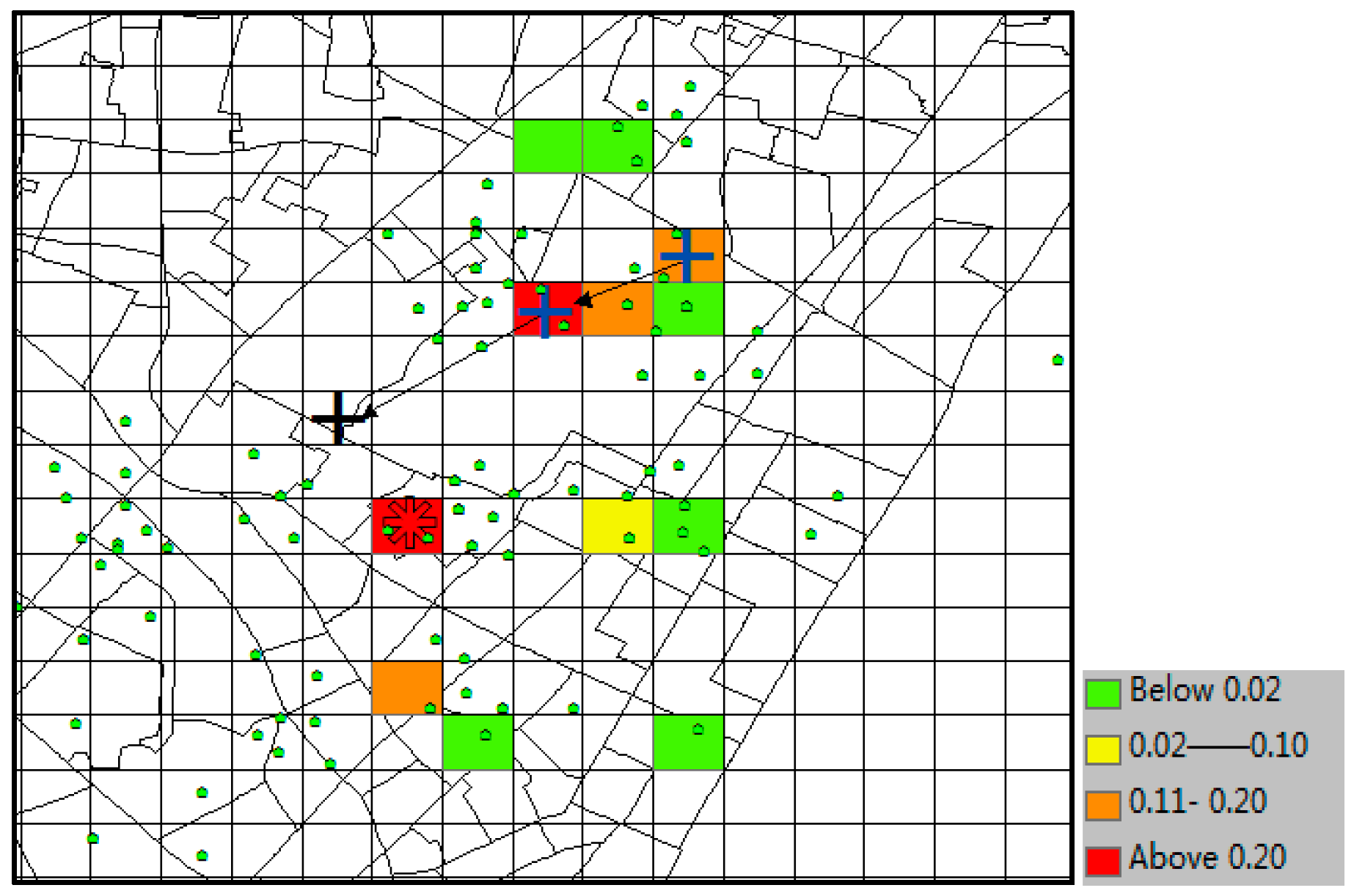
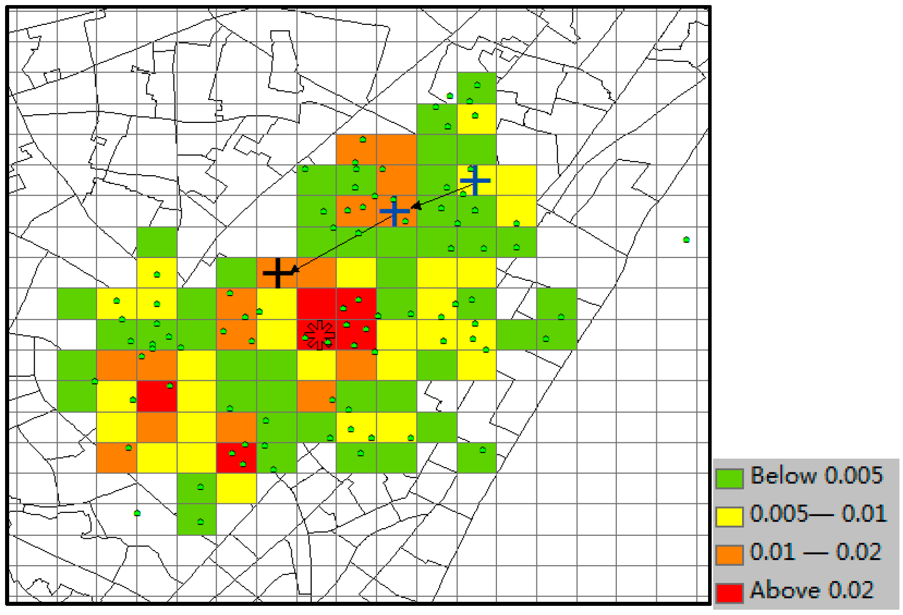
4.8. Visualizations of Prediction Results

This section gives visualization examples of the four models for one prediction test using the same dataset.

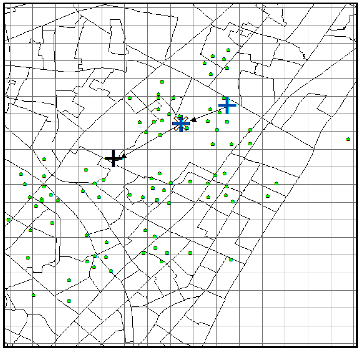
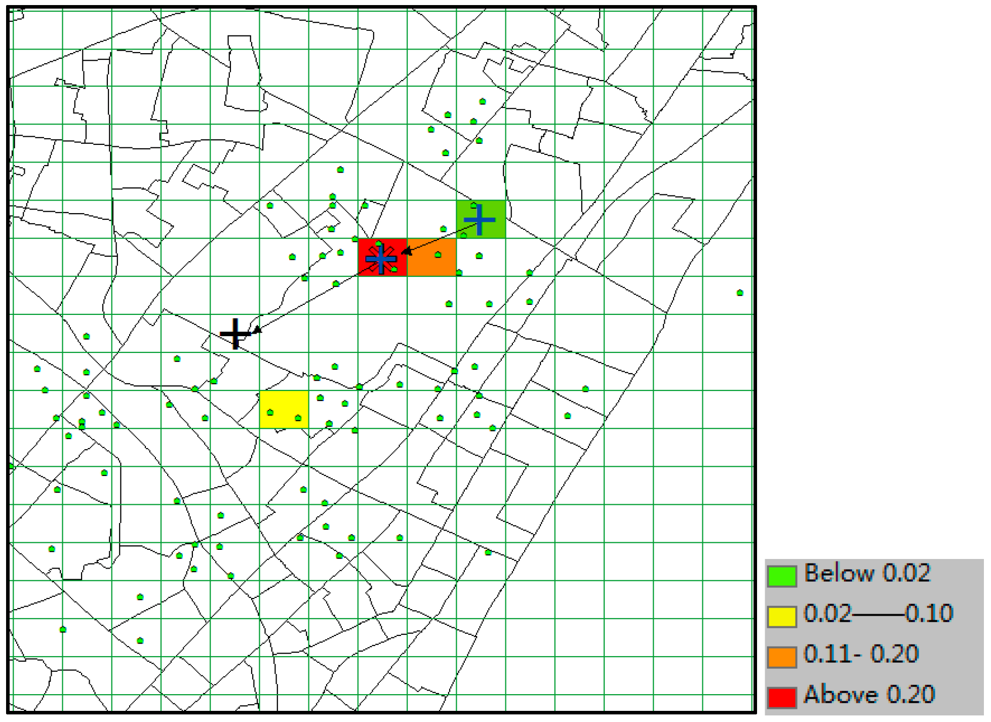
The predicted result of CMoB is shown in Figure 16, where the little green dots represent the visiting venues of the target suspect and his/her similar suspects (some dots overlap with each other), the query trajectory is composed of blue “+” and black arrows, and the colored grid denotes the predicted locations with the probabilities in decreasing order according to red-orange-yellow-green. The symbol “*” denotes the predicted location with highest probability, and the correct destination is represented as the black “+”, which is included in the predicted result set as the 8th highest probability. In this experiment, when k ≥ 8, this can be considered as a correct time with its TE = 0 m. From the plot, we can discover that the correct destination was an unobserved location that is never visited by the suspects, though it was still selected among the candidate predicted locations due to the outstanding ability of our model to learn transition frequencies of unobserved locations from sparse mobility data.

With the same prediction condition, the predicted results of SubSyn are shown in Figure 17. From the plot, we can see that this model is unable to include the correct destination (black “+”) into its prediction result set (no color in that grid). Therefore, when k ≥ 8, this cannot be considered as a correct time, and its TE is 300 m (the distance between the grids of black “+” and “*”).

With the same prediction condition, the predicted results of ZMDB are shown in Figure 18. Because there is no trajectory in the dataset containing the query trajectory (2 blue symbols of “+” ) with the number of trajectory points being greater than 2, the prediction result set is empty (no grid is colored). Thus, the grid of the last point (the grid covering both blue “+” and “*”) in the query trajectory was considered as the unique candidate predicted location. Hence, when k ≥ 8, it would not be a correct time, and its TE is 700 m (the distance between the grid covering black “+” and the grid covering both of blue “+” and “*”).

The predicted result of Markov is shown in Figure 19. Due to the sparse data, the number of candidate predicted locations (colored grid) is merely four. The model did not incorporate the correct destination (grid of black “+”) into its result set. Therefore, when k ≥ 8, it would not be a correct time, and its TE = 300 m (the distance between the yellow grid and grid of black “+”).

5. Conclusions

This study presents an approach to effectively help police break cases by searching for the spatial correlation of crime locations with the predicted movements of numerous suspects, or it can be used to obtain an early warning of suspects’ abnormal movements if some individual suspects are predicted to leave for high risk areas. However, subject to the sparsity of mobile data, it is challenging to develop an effective location prediction model for an individual suspect using the existing algorithms [60,61,62,63]. In this paper, we propose a novel CMoB model to address this issue based on the spatiotemporal semantics. In particular, this model obtains the suspect group with similar movement preferences according to spatiotemporal semantics. Then, the mobility data of suspects in this group are fused together to learn the transition frequencies of peripheral locations surrounding trajectory locations by a KDE smoothing method based on spatial proximities and spatial semantics. The first-order transition matrix and total transition probabilities between locations are formulated, and the Bayes-based location prediction is realized.

Experiments using real datasets showed that the proposed CMoB has outstanding predictive power compared with other methods on the metrics of top-k error, top-k precision, and missing percentiles, confirming that the proposed model is better and applicable to suspect location prediction. The declining effectiveness of the baseline methods relies mainly on two aspects. First, the sparsity of mobile data seriously undermines their robustness such that they cannot generalize to predict locations in unobserved areas. Most of the time, they can only consider the last point in the query trajectory as a single prediction result. Although SubSyn employs the trajectory data from more suspects and has better robustness compared with ZMDB and Markov, the incorporation of mobility data of un-similar suspects makes the transition patterns largely deviate from those of the target suspect, which has a negative effect on the precision of SubSyn. In comparison, our CMoB effectively lowers the negative impact caused by the sparsity of data by forcing the combination of the trajectory data of similar suspects as data sources and revealing the transition frequencies for unobserved locations based on the spatiotemporal semantics. Such efforts help reveal the comprehensive transition patterns of the target suspect and thus maintain a stable performance to advance its effectiveness by obtaining more predicted candidate locations close to the correct destinations.

The ideas suggested in this paper also play important roles in a large number of applications that require the prediction of locations from sparse observed data, such as prediction of the next terrorist attack, estimation of the commercial venue for users, prediction of the locations of enemy troops or discovery of victims in earthquake disasters. In the future, this study needs to be extended to other cities and areas where the size of the individual geo-crime data is small and thus could be biased. In this manner, the flexibility of the proposed model can further be explored. Further improvement could be achieved by employing more features, for example, leveraging suspects’ temporal preferences, personalized information, dynamical geo-social data or urban ubiquitous data, such as 110 calling data (emergence-request service data in China). A second possible improvement could be resorting to more complex prediction models, such as deep neural networks, which can conduct automatic feature abstraction and represent the strong non-linear correlation among original features. In addition, the predicted location profiles can be further enriched, which will be beneficial for the semantic locations (e.g., POI type) prediction or the next offending location estimation.