
LandXML Encoding of Mixed 2D and 3D Survey Plans with Multi-Level Topology †


Abstract
:1. Introduction
Methodology
2. Background
2.1. Survey Plans
2.2. Topology in Cadastral Data
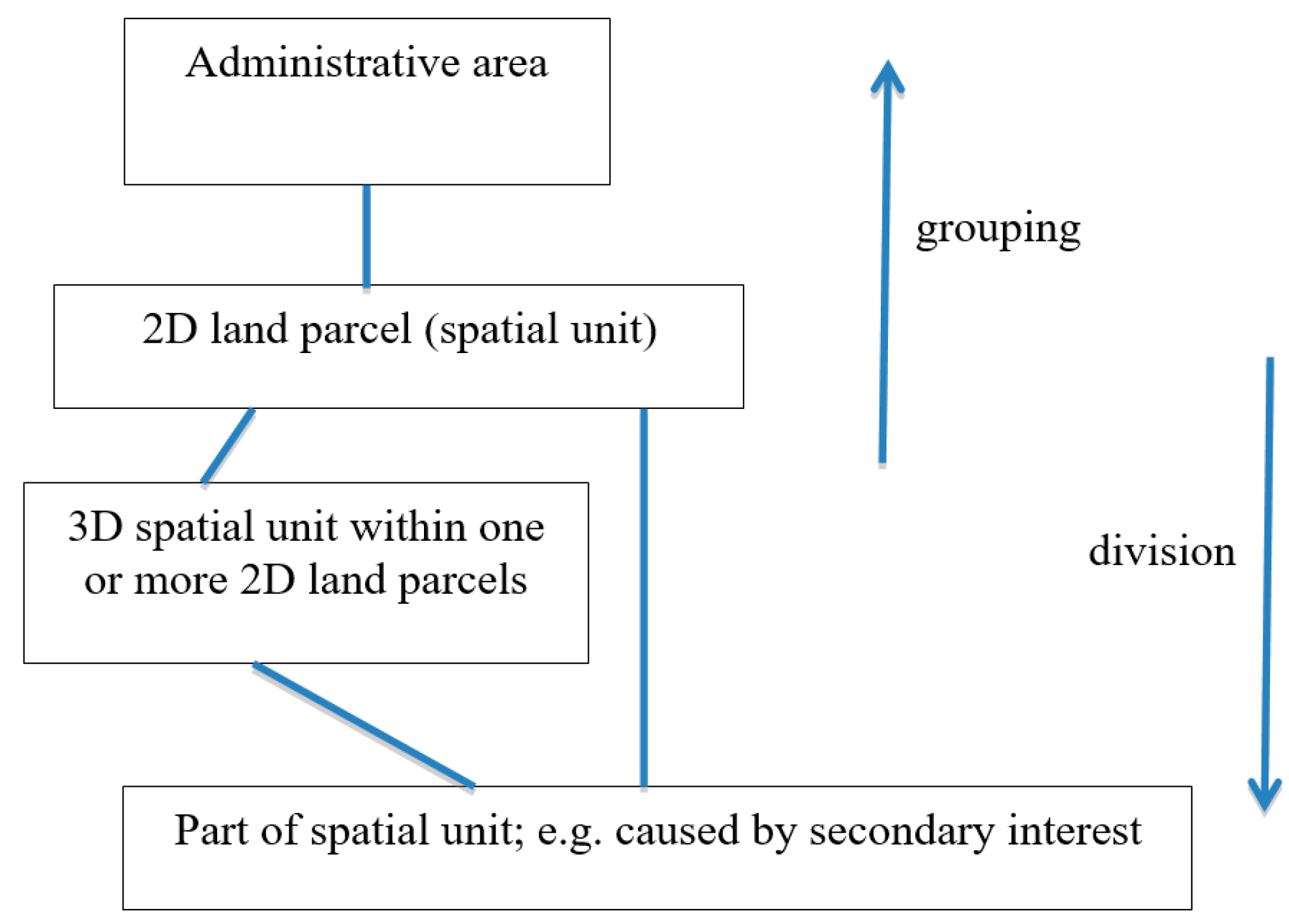
3. Topological Representation of 2D and 3D Spatial Units
- The 2D Land Parcel;
- The Building Format Unit (where the definition of the parcel is the actual building walls);
- The Polygonal Slice (where the units are described by vertical planes, with height limits);
- The Single-Valued Stepped Slice (where all surfaces are vertical or horizontal, and the unit does not have parts overlying other parts);
- The Multi-Valued Stepped Slice (where all surfaces are vertical or horizontal, but parts may overlie others); and
- General 3D Parcels (with few restrictions beyond validity).
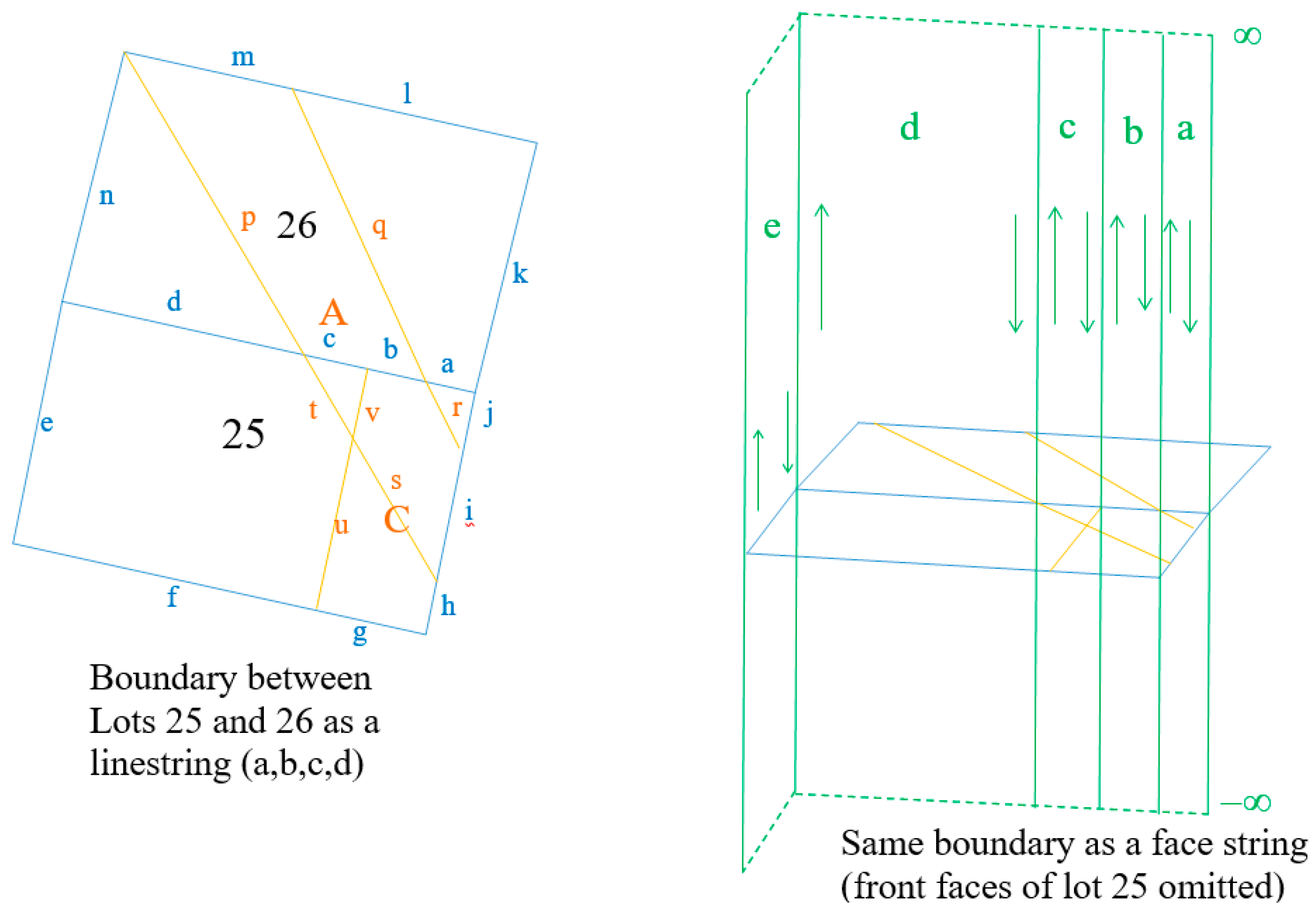
3.1. 2D Cadastral Spatial Unit
- (1)
- Line segment a has Lot 25 and Easement C on left; Lot 26 on right;
- (2)
- Line segment b has Lot 25, Easement A and C on left; Lot 26 and Easement A on right;
- (3)
- Line segment c has Lot 25 and Easement A on left; Lot 26 and Easement A on right;
- (4)
- Line segment d has Lot 25 on left, Lot 26 on right;
- (5)
- Line segment e has Lot 25 on left;
- Therefore, Lot 25 is defined as being on the left of line segments a,b,c,d,e,f,g,h,i,j and both sides of t,s,r,v,u;
- Lot 26 is left of k,l,m,n, right of a,b,c,d and both sides of q,p;
- Easement A is left i and m, right of t,p,q,r,s and both sides of b,c,v.
3.2. Extension to 3D
3.3. Simple 3D Spatial Unit
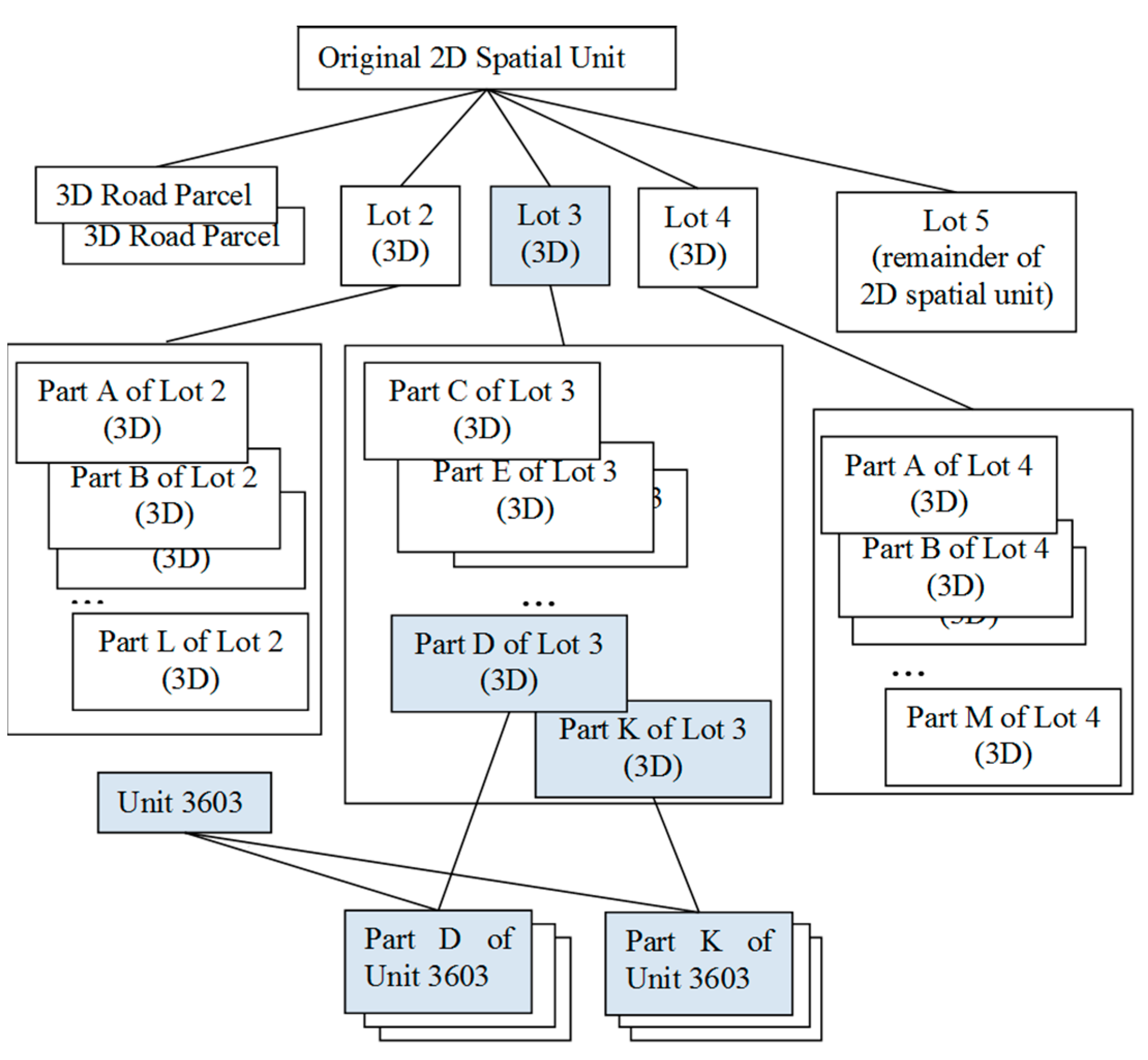
3.4. Complex 3D Spatial Units
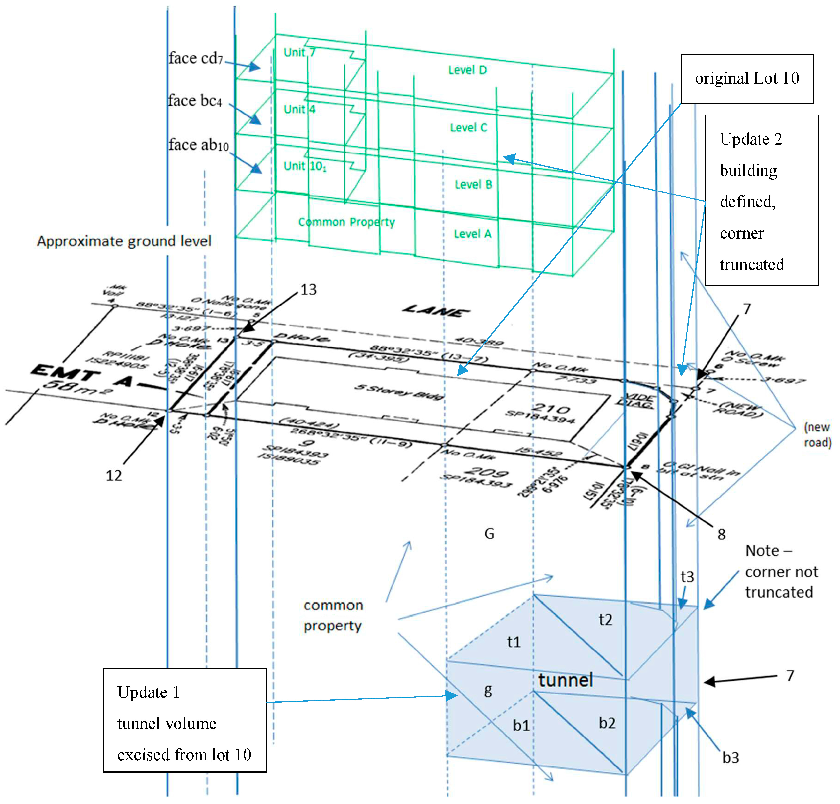
3.5. Multi-Level Case of a Tunnel Below a Building
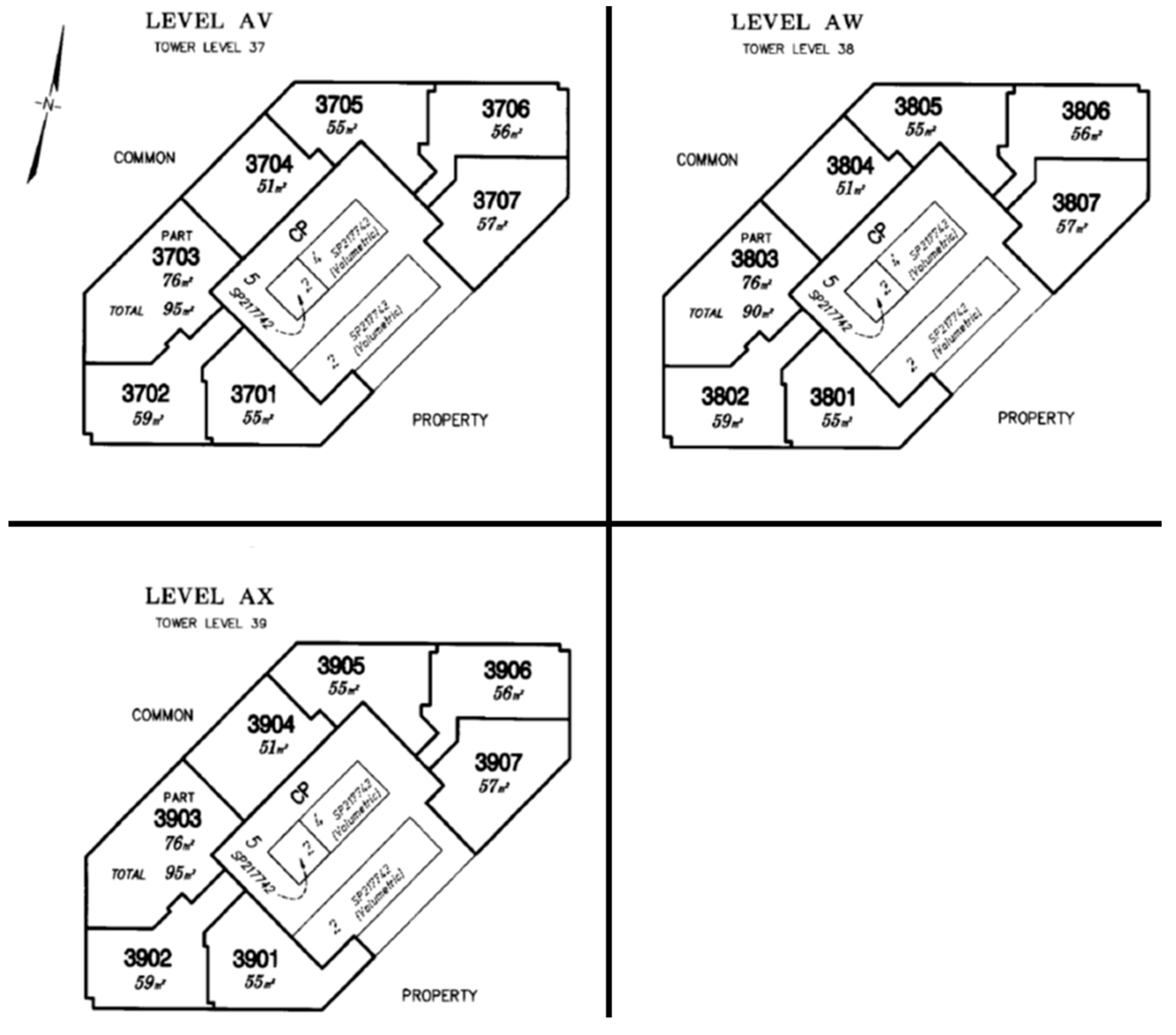
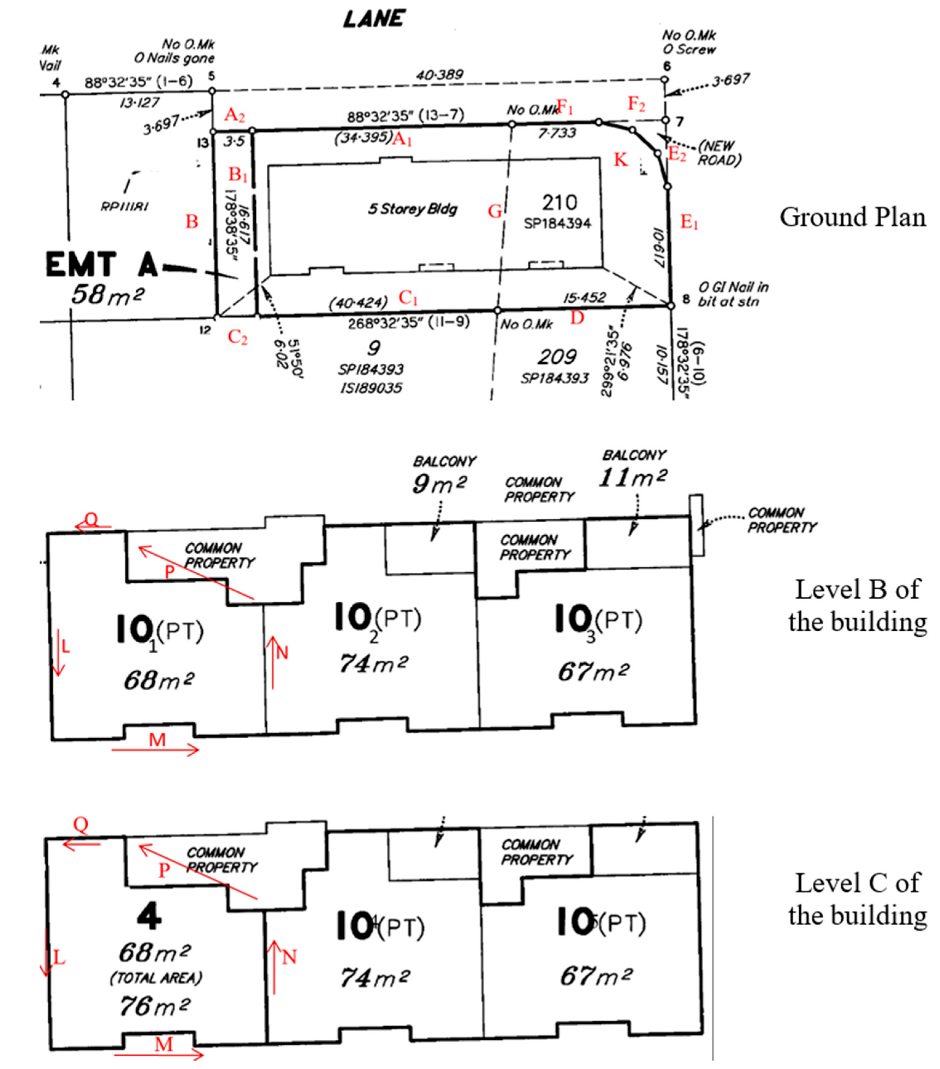
3.6. Multi-Level Hierarchical Case—A High-Rise Building
Lot 3 Part K
4. Representation in LandXML
- Parcel: in LandXML, the term “parcel” is overloaded to include volumes, faces, and face strings. The class attribute of the parcel element makes this explicit (Face, Lot, FaceString, etc.)
- Parcels: Parcels are a collections of parcels that are used to define a higher-level parcel. For example, a set of Faces and FaceStrings that define a volume.
- CoordGeom: Strictly speaking, this defines a chain of straight line segments, but traditionally in LandXML encoding, a closed CoordGeom is assumed to be a planar surface (polygon).
4.1. 2D Cadastral Spatial Units
  <Parcel class=“FaceString” name=“a”>
    <CoordGeom><Line><Start
 pntRef=“1”/><End pntRef=“2”/></Line>
    </CoordGeom></Parcel>
  <Parcel class=“FaceString” name=“b”>
    <CoordGeom><Line><Start pntRef=“2”/><End
 pntRef=“3”/></Line>
    </CoordGeom></Parcel> (etc.)
  <Parcel class=“Lot” name=“25”
 parcelFormat=“Standard”>
    <Parcels>
      <Parcel pclRef=“a”    />    <Parcel
pclRef=“b”/> (etc.)
      <Parcel pclRef=“i”/> (etc.)
    </Parcels>
  </Parcel>
  <Parcel class=“Lot” name=“26”
 parcelFormat=“Standard”>
    <Parcels>
      <Parcel pclRef=“a”
 />       <Parcel pclRef=“b”/> (etc.)
      <Parcel pclRef=“k”/> (etc.)
    </Parcels>
   </Parcel>
   <Parcel class=“Easement” name=“A”
 parcelFormat=“Standard”>
      <Parcels>
        <Parcel pclRef=“i” />    <Parcel pclRef=“r”/>
  (etc.)
      </Parcels>
    </Parcel>  … etc.
|
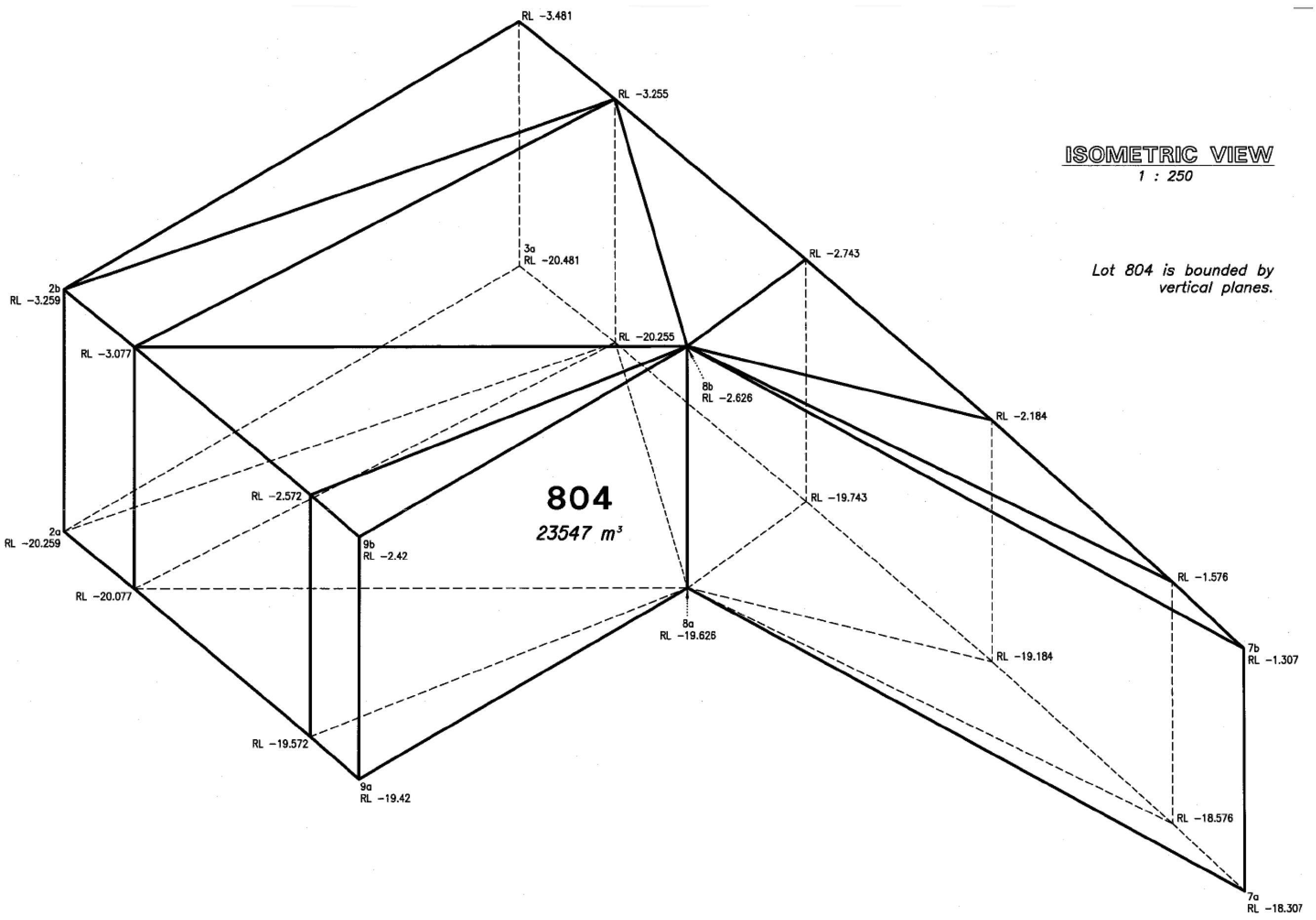
4.2. Simple 3D Spatial Unit
  <Parcel class=“FaceString” name=“U1”>
    <CoordGeom><Line><Start
 pntRef=“2”/><End pntRef=“21”/></Line>
  <Line><Start pntRef=“21”/><End
   pntRef=“22”/></Line>
  <Line><Start pntRef=“22”/><End
 pntRef=“9”/></Line>
    </CoordGeom></Parcel>
  <Parcel class=“FaceString” name=“K1”>
    <CoordGeom><Line><Start
 pntRef=“9”/><End pntRef=“8”/></Line>
    </CoordGeom></Parcel>
  <Parcel class=“FaceString” name=“K2”>
    <CoordGeom><Line><Start
 pntRef=“8”/><End pntRef=“7”/></Line>
    </CoordGeom></Parcel>
  <Parcel class=“Face” name=“t1”>
    <CoordGeom><Line><Start
 pntRef=“2b”/><End pntRef=“74b”/></Line>
      <Line><Start pntRef=“74b”/><End
 pntRef=“3b”/></Line>
      <Line><Start pntRef=“3b”/><End
 pntRef=“2b”/></Line>
  </CoordGeom></Parcel>
  (etc.)
  <Parcel class=“Lot” name=“904”
 parcelFormat=“Volumetric”>
    <Parcels>
   <Parcel pclRef=“U1”/>    <Parcel
    pclRef=“K1”/>
   <Parcel pclRef=“K2”/> (etc.)
   <Parcel pclRef=“t1”/>    <Parcel pclRef=“t2”/>
      (etc.)
    </Parcels>
  </Parcel>
  <Parcel class=“Road” parcelFormat=“Standard”>
    <Parcels>
       <Parcel pclRef=“K1” />    <Parcel pclRef=“K2”/>
 (etc.)
       <Parcel pclRef=“¬t1”/>
    <Parcel pclRef=“¬t2”/>
  <Parcel pclRef=“u1”/>  (etc.)
    </Parcels>
  </Parcel>
  etc.
|
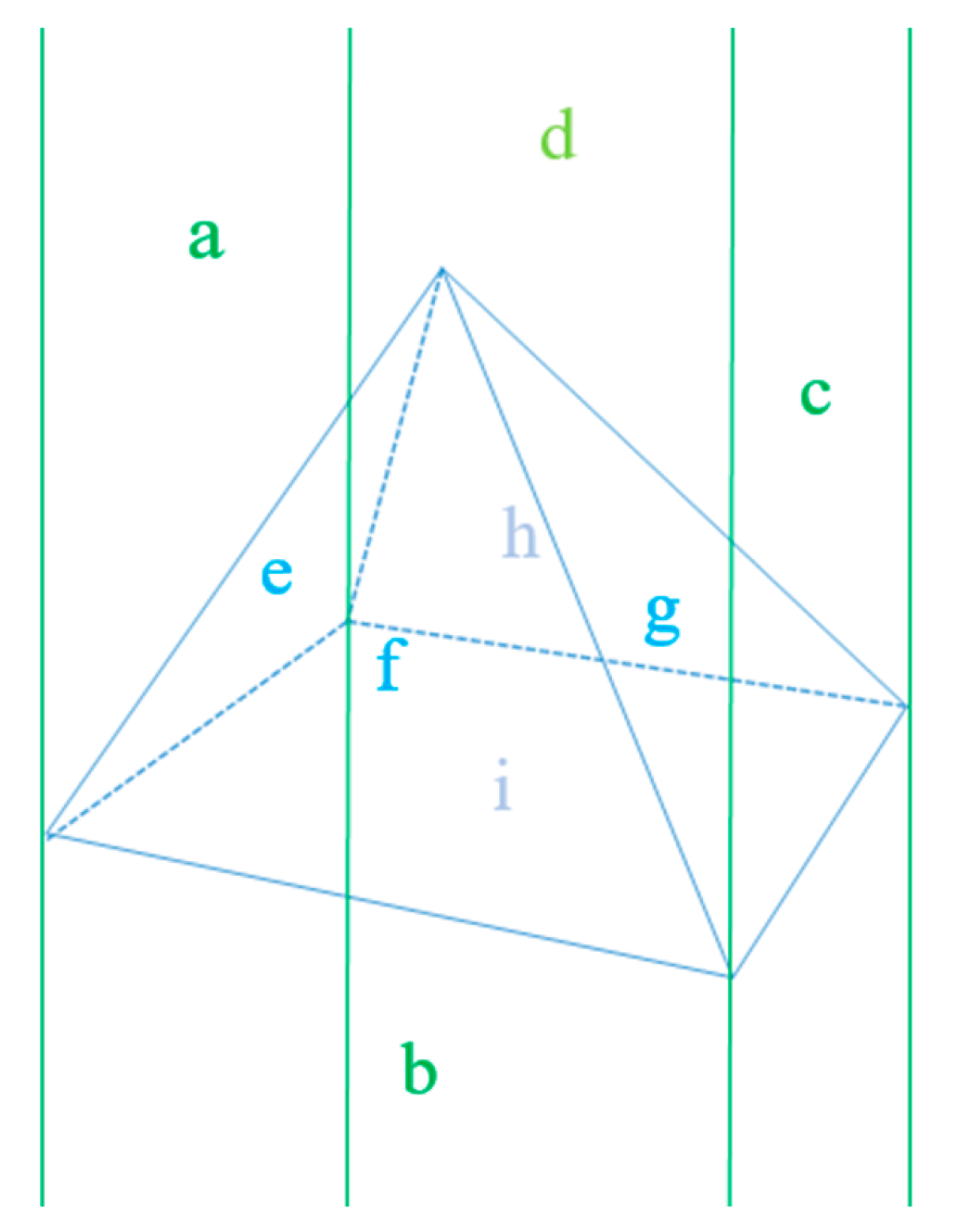
4.3. Complex 3D Spatial Units
  <Parcel class=“FaceString” name=“a”>
    <CoordGeom> detail
 </CoordGeom></Parcel>
  <Parcel class=“FaceString” name=“b”>
    <CoordGeom> detail
 </CoordGeom></Parcel>
  <Parcel class=“FaceString” name=“c”>
    <CoordGeom> detail
 </CoordGeom></Parcel>
  <Parcel class=“FaceString” name=“d”>
    <CoordGeom> detail
 </CoordGeom></Parcel>
  <Parcel class=“Face” name=“e”>
    <CoordGeom> detail
 </CoordGeom></Parcel>
  <Parcel class=“Face” name=“f”>
    <CoordGeom> detail
 </CoordGeom></Parcel>
  <Parcel class=“Face” name=“g”>
    <CoordGeom> detail
 </CoordGeom></Parcel>
  <Parcel class=“Face” name=“h”>
    <CoordGeom> detail
 </CoordGeom></Parcel>
  <Parcel class=“Face” name=“i”>
    <CoordGeom> detail
 </CoordGeom></Parcel>
  <Parcel class=“Lot” name=“L1”
 parcelFormat=“Volumetric”>
    <Parcels>
      <Parcel pclRef=“a”/>    <Parcel
    pclRef=“b”/>
      <Parcel pclRef=“c”/>    <Parcel
    pclRef=“d”/>
      <Parcel pclRef=“e”/>    <Parcel
    pclRef=“f”/>
      <Parcel pclRef=“g”/>    <Parcel
    pclRef=“h”/>
      <Parcel pclRef=“i”/>
    </Parcels>
  </Parcel>
  <Parcel class=“Lot” name=“Common
 Property” parcelFormat=“Standard”>
    <Parcels>
      <Parcel pclRef=“a”/>    <Parcel
    pclRef=“b”/>
      <Parcel pclRef=“c”/>    <Parcel
    pclRef=“d”/>
      <Parcel pclRef=“e”/>
< Parcel pclRef=“f”/>
      <Parcel pclRef=“g”/>
<Parcel pclRef=“h”/>
      <Parcel pclRef=“i”/>
    </Parcels>
  </Parcel>
  etc.
|
4.4. Case of a Tunnel Below a Building (from Section 3.5)
4.5. Multi-Level Hierarchical Case—High-Rise Building from Section 3.6
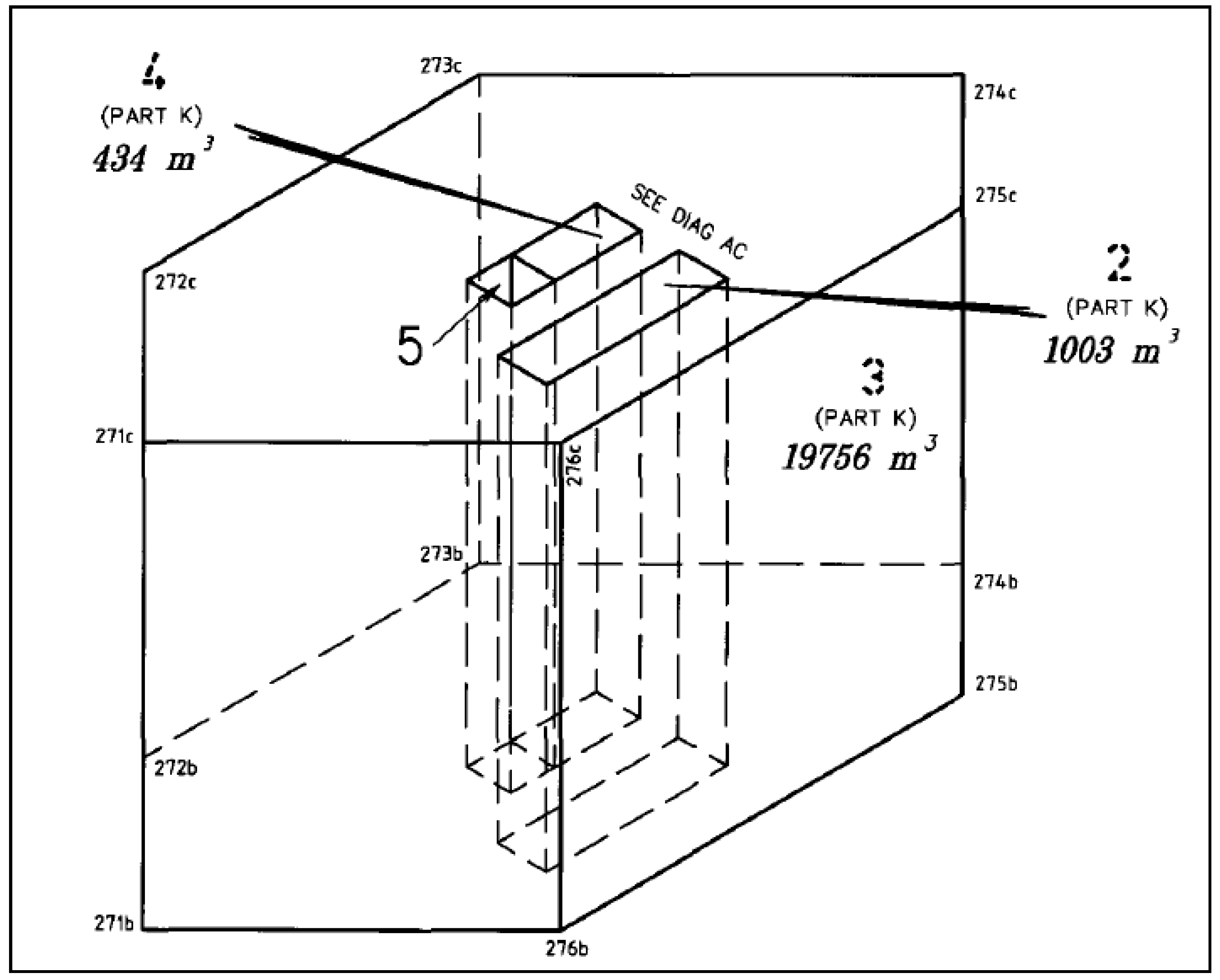
4.5.1. Encoding of Lot 3 Part K
  <Parcel class=“FaceString”
name=“TowerOuter”>
    <CoordGeom><Line><Start
pntRef=“271”/><End pntRef=“276”/></Line>
      <Line><Start
pntRef=“276”/><End pntRef=“275”/></Line>
      <Line><Start
pntRef=“275”/><End pntRef=“274”/></Line>
      <Line><Start
pntRef=“274”/><End pntRef=“273”/></Line>
      <Line><Start
pntRef=“273”/><End pntRef=“272”/></Line>
      <Line><Start
pntRef=“272”/><End pntRef=“271”/></Line>
    </CoordGeom></Parcel>
  <Parcel class=“FaceString”
name=“LiftWell5Inner”>
    <CoordGeom><Line><Start
pntRef=“23”/><End pntRef=“20”/></Line>
      <Line><Start
pntRef=“20”/><End pntRef=“21”/></Line>
      <Line><Start
pntRef=“21”/><End pntRef=“22”/></Line>
      <Line><Start
pntRef=“22”/><End pntRef=“23”/></Line>
    </CoordGeom></Parcel>
|
  <Parcel class=“Face” name=“KTop”>
    <CoordGeom><Line><Start
pntRef=“271b”/><End pntRef=“276b”/></Line>
      <Line><Start
pntRef=“276b”/><End pntRef=“275b”/></Line>
      <Line><Start
pntRef=“275b”/><End pntRef=“274b”/></Line>
      <Line><Start
pntRef=“274b”/><End pntRef=“273b”/></Line>
      <Line><Start
pntRef=“273b”/><End pntRef=“272b”/></Line>
      <Line><Start pntRef=“272b”/><End
pntRef=“271b”/></Line>
  </CoordGeom></Parcel>
|
<Parcel class=“Face” name=“KTop” a=“0” b=“0” c=“-1” d=“137.625”/> |
    <Parcel class=“FaceString”
name=“LiftWell2Outer”>
  <CoordGeom><Line><Start
pntRef=“25”/><End pntRef=“24”/></Line>
    <Line><Start
pntRef=“24”/><End pntRef=“28”/></Line>
    <Line><Start
pntRef=“28”/><End pntRef=“29”/></Line>
    <Line><Start
pntRef=“29”/><End pntRef=“25”/></Line>
  </CoordGeom></Parcel>
<Parcel class=“FaceString”
name=“LiftWell4Outer”>
  <CoordGeom><Line><Start
pntRef=“23”/><End pntRef=“132”/></Line>
     <Line><Start
pntRef=“132”/><End pntRef=“131”/></Line>
     <Line><Start
pntRef=“131”/><End pntRef=“22”/></Line>
     <Line><Start
pntRef=“22”/><End pntRef=“23”/></Line>
  </CoordGeom></Parcel>
|
  <Parcel class=“LOT” name=“3K”
parcelFormat=“Volumetric”>
    <Parcels>
      <Parcel pclRef=“TowerOuter”/>
<Parcel pclRef=“LiftWell5Inner”/>
      <Parcel pclRef=“KTop”/>
<Parcel pclRef=“JTop” />
      <Parcel pclRef=“¬LiftWell2Outer”/>
        <Parcel pclRef=“¬LiftWell4Outer”/>
    </Parcels>
|
  <Parcel class=“FaceString”
name=“Lot5Outer”>
    <CoordGeom> (the definition of the
original 2D lot as a footprint face string)
    </CoordGeom></Parcel>
  <Parcel class=“LOT” name=“5”
parcelFormat=“Volumetric”>
    <Parcels>
      <Parcel pclRef=“Lot5Outer” />
<Parcel pclRef=“-4” />
      <Parcel pclRef=“-3”/>
<Parcel pclRef=“-2” />
      <Parcel pclRef=“-Road” />  ...
    </Parcels>
  </Parcel>
|
4.5.2. Encoding the Units within Lot 3
  <Parcel class=“LOT” name=“3701U”
parcelFormat=“Building”>
    <Parcels>
      <Parcel pclRef=“Unit3101-3102” />
<Parcel pclRef=“Unit3101Outer”/>
      etc.
      <Parcel pclRef=“36Top”/>
<Parcel pclRef=“37Top”/>
     </Parcels>
  </Parcel>
  <Parcel class=“LOT” name=“3801U”
parcelFormat=“Building”>
    <Parcels>
      <Parcel pclRef=“Unit3101-3102” />
<Parcel pclRef=“Unit3101Outer”/>
      etc.
      <Parcel pclRef=“¬37Top”/>
<Parcel pclRef=“38Top”/>
    </Parcels>
  </Parcel>
|
  <Parcel class=“LOT” name=“3201”
parcelFormat=“Building”>
    <Parcels>
      <Parcel pclRef=“+3201U” />
<Parcel pclRef=“+3201P”/>
    </Parcels>
  </Parcel>
|
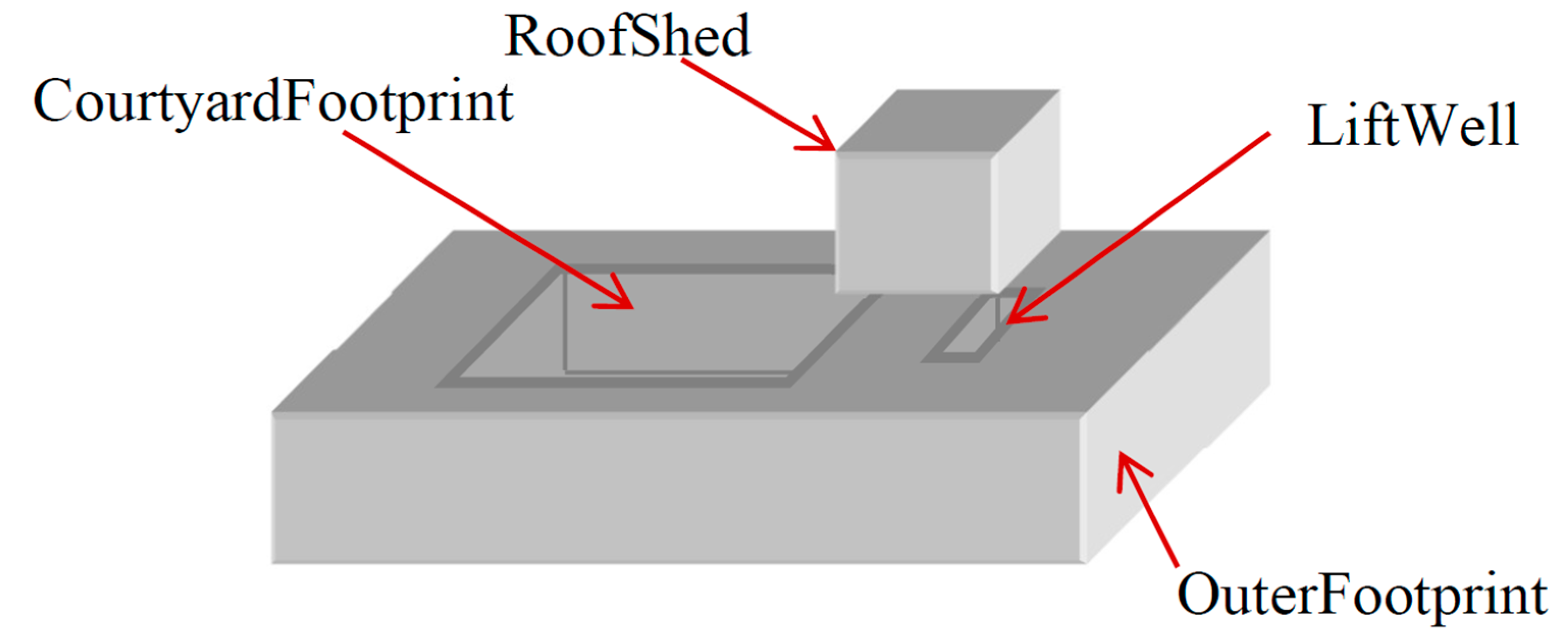
4.6. Spatial Logic Issues
  <Parcel class=“LOT” name=“L”
parcelFormat=“Volumetric”>
    <Parcels>
      <Parcel pclRef=“OuterFootprint”/>
      <Parcel
pclRef=“CourtyardFootprint”/>
      <Parcel pclRef=“Top1”/>
<Parcel pclRef=“¬Top2” />
      <Parcel pclRef=“-LiftWell”/>
<Parcel pclRef=“+RoofShed”/>
    </Parcels>
  </Parcel>
|
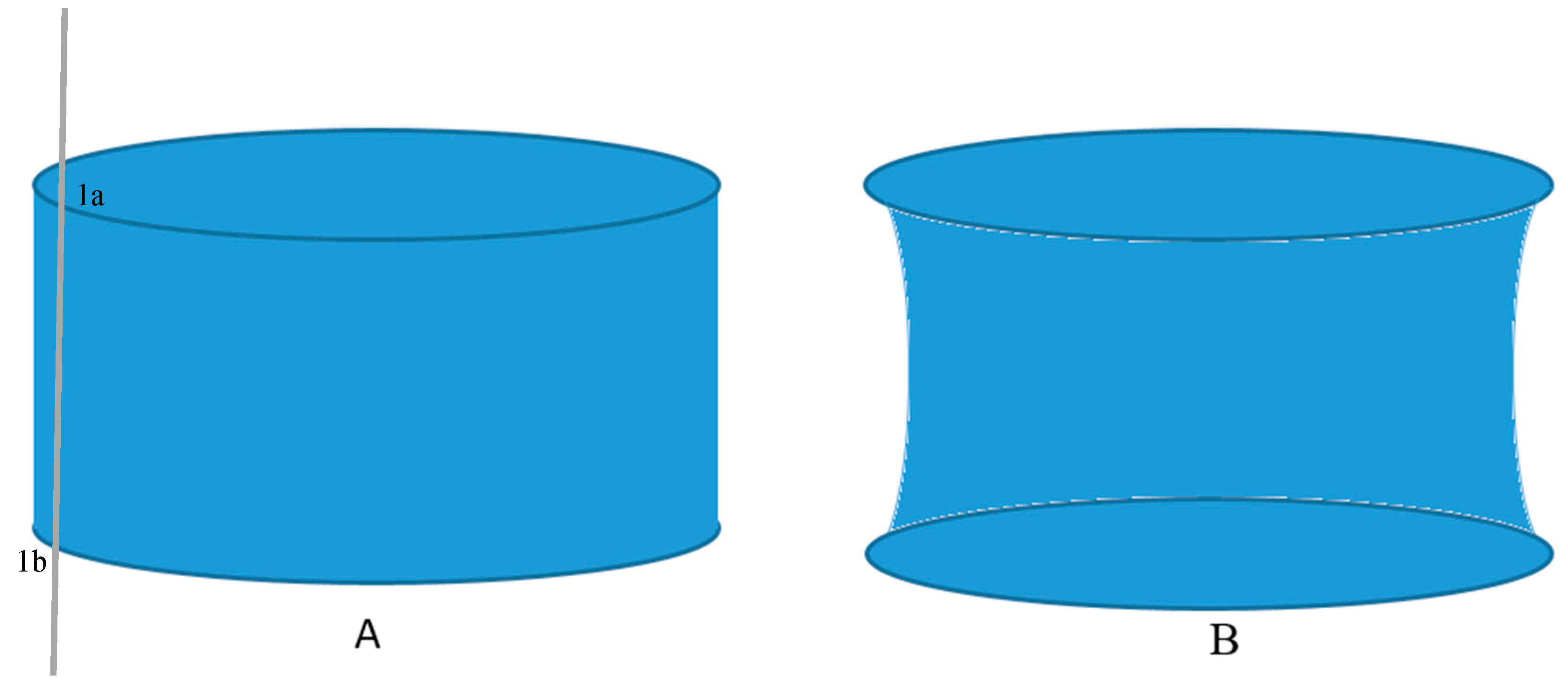
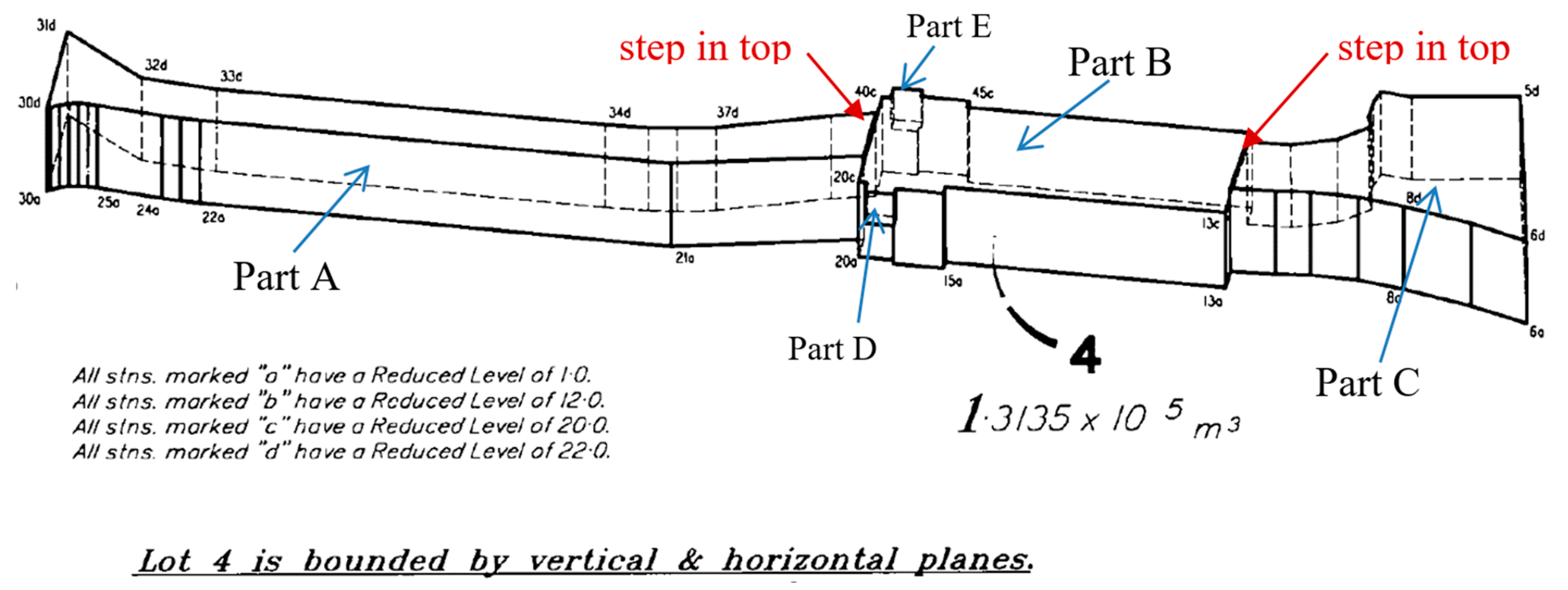
4.7. Curved Surfaces
  <Parcel class=“FaceString”
name=“Outer”>
    <CoordGeom><Curve radius=“25”
rot=“acw”>
      <Start pntRef=“1”/><End
pntRef=“1”/></Curve>
    </CoordGeom></Parcel>
  <Parcel class=“Face” name=“Top” a=“0”
b=“0” c=“-1” d=“130”/> <Parcel class=“Face” name=“Bottom” a=“0” b=“0”
c=“1” d=“-120”/>
|
4.8. Alternate Encodings
5. Implementation Issues
5.1. Completeness of Implementation
5.2. Conversion to Polyhedron Form
5.3. Conversion from Polyhedra Form
- (1)
- The parameters (a,b,c,d) of each face are calculated. This is not trivial, involving a least-squares fitting of the function aX + bY + cZ + d to the set of vertices of the face, but this is a necessary action in any case to validate the face. Where c < 0, this is a top face, and it is replaced by a 2D polygon, with Z = 0 for each vertex. Where c ≥ 0, the face is discarded.
- (2)
- These polygons are then dissolved to produce a (multi) polygon (with possible holes). This becomes the footprint boundary face string.
- (3)
- The faces are then re-scanned, and any with c = 0 are tested against the boundary face string. If they fall within it, they are discarded. Otherwise, they are retained, along with all faces with c ≠ 0, as boundary faces.
- (4)
- This produces a non-topological encoding of the spatial units of the plan. Normal 2D algorithms can be used to convert the face strings to a topological network that encodes the individual spatial units in 2D. In a similar way, shared faces can be detected and encoded.
5.4. Viewing and Manipulating Data Using 2D Software
5.5. Calculations and Rounding Errors
6. Analysis of Results
6.1. Sharing of Data
- Some definitions are not shared: Face strings at the edge of the plan, and faces that surround a secondary interest (not excised from the enclosing spatial unit) are examples.
- Many definitions are shared by exactly two spatial units—where they form the boundary between them.
- A significant number of face strings are shared a large number of times: For example, the face string “Unit3101–3102” defined in Section 4.5.2 would be used in the units 3101 to 3910 (9 units), and reversed in 3102 to 3902. A total of 18 usages.
7. Conclusions and Future Research
7.1. Major Results
- It is a close fit to current cadastral survey practice (Section 3.2).
- It permits efficient encoding, explicit semantics on neighbors, reduction of redundancy, and avoids inconsistencies. (Section 6.1)
- It is capable of being viewed and even manipulated by software that is strictly 2D (not 3D-aware) (see Section 5.4).
7.2. Future Work
Author Contributions
Conflicts of Interest
References
- Lemmen, C.; van Oosterom, P.; Thompson, R.J.; Hespanha, J.; Uitermark, H. The Modelling of Spatial Units (Parcels) in the Land Administration Domain Model (LADM). In Proceedings of the XXIV FIG International Congress, Sydney, Australia, 11–16 April 2010. [Google Scholar]
- ISO TC211. ISO 19152:2012 Geographic Information—Land Administration Domain Model (LADM). Available online: https://www.iso.org/standard/51206.html (accessed on 6 May 2017).
- Thompson, R.J.; van Oosterom, P.; Soon, K.H.; Priebbenow, R. A Conceptual Model Supporting a Range of 3D Parcel Representations through all Stages: Data Capture, Transfer and Storage. In Proceedings of the FIG Working Week 2016, Christchurch, New Zealand, 2–6 May 2016. [Google Scholar]
- LandXML. Available online: http://www.landxml.org/ (accessed on 6 May 2017).
- Scarponcini, P. InfraGML Proposal (13–121), OGC Land and Infrastructure Domain Working Group. Available online: https://portal.opengeospatial.org/files/?artifact_id=56299 (accessed on 6 May 2017).
- OGC InfraGML 1.0. Available online: https://portal.opengeospatial.org/files/?artifact_id=72352 (accessed on 6 May 2017).
- Thompson, R.; van Oosterom, P. Axiomatic Definition of Valid 3D Parcels, Potentially in a Space Partition. In Proceedings of the 2th International FIG 3D Cadastre Workshop, Delft, The Netherlands, 16–18 November 2011. [Google Scholar]
- Thompson, R.; van Oosterom, P.; Karki, S.; Cowie, B. A Taxonomy of Spatial Units in a Mixed 2D and 3D Cadastral Database. In Proceedings of the FIG Working Week 2015, Sofia, Bulgaria, 17–21 May 2015. [Google Scholar]
- Thompson, R.J.; van Oosterom, P.; Soon, K.H. Mixed 2D and 3D Survey Plans with Topological Encoding. In Proceedings of the 5th International FIG 3D Cadastre Workshop, Athens, Greece, 18–20 October 2016. [Google Scholar]
- ICSM. ePlan Data Model Governance. Available online: http://www.icsm.gov.au/eplan/ePlan_Governance_v1.1.pdf (accessed on 6 May 2017).
- Janečka, K.; Karki, S. 3D Data Management—Overview Report. In Proceedings of the 5th International FIG 3D Cadastre Workshop, Athens, Greece, 18–20 October 2016. [Google Scholar]
- Dimipoulou, E.; Karki, S.; Miodrag, R.; de Almeida, J.-P.D.; Griffith-Charles, C.; Thompson, R.; Ying, S.; van Oosterom, P. Initial Registration of 3D Parcels: Overview Report. In Proceedings of the 5th International FIG 3D Cadastre Workshop, Athens, Greece, 18–20 October 2016. [Google Scholar]
- Soon, K.H.; Tan, D.; Khoo, V. Initial Design to Develop a Cadastral System that Supports Digital Cadastre, 3D and Provenance for Singapore. In Proceedings of the 5th International FIG 3D Cadastre Workshop, Athens, Greece, 18–20 October 2016. [Google Scholar]
- Zeiss, G. A Proposal to Replace LandXML with a New Standard: InfraGML. Directions Magazine 11th Dec. 2013. Available online: http://www.directionsmag.com/entry/a-proposal-to-replace-landxml-with-a-new-standard-infragml/371892 (accessed on 6 May 2017).
- Stoter, J.E.; van Oosterom, P. 3D Cadastre in an International Context: Legal, Organizational, and Technological Aspects; CRC Press: Boca Raton, FL, USA, 2006; p. 344. [Google Scholar]
- Oldfield, J.; van Oosterom, P.; Quak, W.; van der Veen, J.; Beetz, J. Can Data from BIMs be Used as Input for a 3D Cadastre? In Proceedings of the 5th International FIG 3D Cadastre Workshop. Athens, Greece, 18–20 October 2016. [Google Scholar]
- Paulsson, J. Sweedish 3D Property in an International Comparison. In Proceedings of the 3rd International FIG 3D Cadastre Workshop: Developments and Practices, Shenzhen, China, 25–26 October 2012. [Google Scholar]
- Atazadeh, B.; Kalantari, M.; Rajabifard, A.; Ho, S.; Ngo, T. Building Information Modelling for High-rise Land Administration. Trans. GIS 2017, 21, 91–113. [Google Scholar] [CrossRef]
- Van Oosterom, P.; Stoter, J.; Quak, W.; Zlatanova, S. The Balance between Geometry and Topology. In Advances in Spatial Data Handling; Richardson, D.E., van Oosterom, P., Eds.; Springer: Berlin/Heidelberg, Germany, 2002; pp. 209–224. [Google Scholar]
- Hoel, E.; Menon, S.; Morehouse, S. Building a Robust Relational Implementation of Topology. In Lecture Notes in Computer Science: Advances in Spatial and Temporal Databases. SSTD 2003; Hadzilacos, T., Manolopoulos, Y., Roddick, J., Theodoridis, Y., Eds.; Springer: Berlin/Heidelberg, Germany, 1993; Volume 2750, pp. 508–524. [Google Scholar]
- Louwsma, J. H. Topology Versus Non-Topology Storage Structures. Available online: http://www.gdmc.nl/publications/2003/Topology_storage_structures.pdf (accessed on 6 May 2017).
- De Hoop, S.; van Oosterom, P.; Molenaar, M. Topological Querying of Multiple Map Layers. In Lecture Notes in Computer Science: Spatial Information Theory A Theoretical Basis for GIS. COSIT 1993; Frank, A.U., Campari, I., Eds.; Springer: Berlin/Heidelberg, Germany, 1993; Volume 716, pp. 139–157. [Google Scholar]
- Ledoux, H.; Gold, C. Simultaneous Storage of Primal and Dual Three-Dimensional Subdivisions. Comput. Environ. Urban Syst. 2007, 31, 393–408. [Google Scholar] [CrossRef]
- Boguslawski, P.; Gold, C. Construction Operators for Modelling 3D Objects and Dual Navigation Structures. In Lecture Notes in Geoinformation and Cartography: 3D Geoinformation Sciences; Zlatanova, S., Lee, J., Eds.; Springer: Berlin/Heidelberg, Germany, 2009; Part II; pp. 47–59. [Google Scholar]
- Baumgart, B.G. Winged Edge Polyhedron Representation. Stanfort Artificial Intelligence Project, 1972, 44, Document STAN-CS-72-320 Memo AIM-179. Available online: http://www.dtic.mil/dtic/tr/fulltext/u2/755141.pdf (accessed on 6 May 2017).
- Molenaar, M. Single Valued Vector Maps—A Concept in Geographic Information Systems. GeoInform. Syst. 1989, 2, 18–27. [Google Scholar]
- Van Oosterom, P. Research Issues in Integrated Querying of Geometric and Thematic Cadastral Information (2); Technical Report; Delft University of Technology: Delft, The Netherlands, 2000. [Google Scholar]
- DNRM Cadastral Survey Requirements v7.1, Reprint 1. Department of Natural Resources and Mines, 2016. Available online: https://www.dnrm.qld.gov.au/?a=105601 (accessed on 6 May 2017).
- ICSM. ePlan Protocol LandXML Mapping. Available online: https://icsm.govspace.gov.au/files/2011/09/ePlan-Protocol-LandXML-Mapping-v2.1.pdf (accessed on 6 May 2017).
- Abdel_Malek, K.; Yeh, H.J. Determining Intersection Curves Between Surfaces of Two Solids. Comput. Aided Des. 1996, 28, 539–549. [Google Scholar] [CrossRef]
- Thompson, R.; van Oosterom, P. Modelling and Validation of 3D Cadastral Objects. In Urban and Regional Data Management: UDMS Annual 2011; Zlatanova, S., Ledoux, H., Fendel, E., Rumor, M., Eds.; CRC Press: London, UK, 2012; pp. 7–23. [Google Scholar]
- Thompson, R.J. Towards a Rigorous Logic for Spatial Data Representation. Ph.D. Thesis, Delft University of Technology, Delft, The Netherlands, 2007. [Google Scholar]
- Weinrich, B.E.; Schneider, M. Use of Rational Numbers in the Design of Robust Geometric Primitives for Three Dimensional Spatial Database Systems. In Proceedings of the 13th Annual ACM Workshop on GIS, Bremen, Germany, 4–5 November 2005; pp. 163–172. [Google Scholar]
- Lema, J.A.C. Dual Grid: A Closed Representation Space for Consistent Spatial Databases. Ph.D. Thesis, Universidade da Coruña, Coruña, Spain, 2012. [Google Scholar]
- Lema, J.A.C.; Güting, R.H. Dual grid: A new Approach for Robust Spatial Algebra Implementation. GeoInformatica 2002, 6, 57–76. [Google Scholar] [CrossRef]
- Thompson, R.J.; van Oosterom, P. Connectivity in the Regular Polytope Representation. GeoInformatica 2011, 15, 223–246. [Google Scholar] [CrossRef]
- Belussi, A.; Migliorini, S.; Negri, M.; Pelagatti, G. Establishing Robustness of a Spatial Dataset in a Tolerance-Based Vector Model. Trans. GIS 2016. [Google Scholar] [CrossRef]
- Stolk, P.; Lemmen, C.H.J. Technical aspects of electronics conveyancing. In Proceedings of the 2nd FIG Regional Conference, Marrakech, Morocco, 2–5 December 2003. [Google Scholar]
- Van Oosterom, P.; Lemmen, C.; Uitermark, H.; Boekelo, G.; Verkuijl, G. Land Administration Standardization with focus on Surveying and Spatial Representations. In Proceedings of the ACMS Annual Conference Survey Summit 2011, San Diego, CA, USA, 7–13 July 2011. [Google Scholar]


| Face String | + Spatial Unit(s) | − Spatial Unit(s) |
|---|---|---|
| a | Lot 25 | Lot 26 |
| b | Lot 25 | Lot 26 |
| d | Lot 25 | Lot 26 |
| i | Easement A, Lot 25 | |
| p | Easement A | |
| q | Easement A |
| Line | + Spatial Unit(s) | − Spatial Unit(s) |
|---|---|---|
| A1 | Lot CP | Mark Lane (road) |
| A2 | Lot CP, Easement A | Mark Lane (road) |
| B | Lot CP, Easement A | Lot 1/RP11181 |
| B1 | Easement A | |
| C2 | Lot CP, Easement A | Lot 9/SP184393 |
| C1 | Lot CP | Lot 9/SP184393 |
| D | Lot CP, Lot 210 | Lot 9 and Lot 209/SP184393 |
| E1 | Lot CP, Lot 210 | Main Street (road) |
| E2 | Lot 210, New Road | Main Street (road) |
| F2 | Lot 210, New Road | Mark Lane (road) |
| F1 | Lot CP, Lot 210 | Mark Lane (road) |
| G | Lot 210 | |
| K | Lot CP | New Road |
| L | Unit 10 part 1, Unit 4 | |
| M | Unit 10 part 1, Unit 4 | |
| N | Unit 10 part 1, Unit 4 | Unit 10 part 2, Unit 10 part 4 |
| P | Unit 10 part 1, Unit 4 | |
| Q | Unit 10 part 1, Unit 4 |
| Face | + Spatial Unit(s) | − Spatial Unit(s) |
|---|---|---|
| t1 | Lot 210 | Lot CP |
| t2 | Lot 210 | Lot CP |
| t3 | Lot 210 | New Road |
| b1 | Lot CP | Lot 210 |
| b2 | Lot CP | Lot 210 |
| b3 | New Road | Lot 210 |
| g | Lot 210 | Lot CP |
| ab10 | Unit 10 part 1 | Common Property |
| bc4 | Unit 4 | Unit 10 part 1 |
| cd7 | Unit 7 (not in diagram) | Unit 4 |
© 2017 by the authors. Licensee MDPI, Basel, Switzerland. This article is an open access article distributed under the terms and conditions of the Creative Commons Attribution (CC BY) license (http://creativecommons.org/licenses/by/4.0/).
Share and Cite
Thompson, R.J.; Van Oosterom, P.; Soon, K.H. LandXML Encoding of Mixed 2D and 3D Survey Plans with Multi-Level Topology. ISPRS Int. J. Geo-Inf. 2017, 6, 171. https://doi.org/10.3390/ijgi6060171
Thompson RJ, Van Oosterom P, Soon KH. LandXML Encoding of Mixed 2D and 3D Survey Plans with Multi-Level Topology. ISPRS International Journal of Geo-Information. 2017; 6(6):171. https://doi.org/10.3390/ijgi6060171
Chicago/Turabian StyleThompson, Rodney James, Peter Van Oosterom, and Kean Huat Soon. 2017. "LandXML Encoding of Mixed 2D and 3D Survey Plans with Multi-Level Topology" ISPRS International Journal of Geo-Information 6, no. 6: 171. https://doi.org/10.3390/ijgi6060171