A Post-Rectification Approach of Depth Images of Kinect v2 for 3D Reconstruction of Indoor Scenes

Abstract

3D reconstruction of indoor scenes is a hot research topic in computer vision. Reconstructing fast, low-cost, and accurate dense 3D maps of indoor scenes have applications in indoor robot positioning, navigation, and semantic mapping. In other studies, the Microsoft Kinect for Windows v2 (Kinect v2) is utilized to complete this task, however, the accuracy and precision of depth information and the accuracy of correspondence between the RGB and depth (RGB-D) images still remain to be improved. In this paper, we propose a post-rectification approach of the depth images to improve the accuracy and precision of depth information. Firstly, we calibrate the Kinect v2 with a planar checkerboard pattern. Secondly, we propose a post-rectification approach of the depth images according to the reflectivity-related depth error. Finally, we conduct tests to evaluate this post-rectification approach from the perspectives of accuracy and precision. In order to validate the effect of our post-rectification approach, we apply it to RGB-D simultaneous localization and mapping (SLAM) in an indoor environment. Experimental results show that once our post-rectification approach is employed, the RGB-D SLAM system can perform a more accurate and better visual effect 3D reconstruction of indoor scenes than other state-of-the-art methods.

1. Introduction

Indoor robot positioning, navigation, and semantic mapping depend on an accurate and robust 3D reconstruction of indoor scenes. A variety of techniques for 3D reconstruction of indoor and outdoor scenes have been developed, such as light detection and ranging (LiDAR) [1], stereo cameras [2], RGB and depth (RGB-D) cameras [3], and so on. Although a three-dimensional LiDAR could satisfy accuracy and robustness, such a system is very costly. Furthermore, the result is short of the important color information [1]. Stereo cameras can be utilized for 3D reconstruction of indoor scenes with low accuracy and a complex processing procedure [4]. Recently, the RGB-D camera has become a better alternative for 3D reconstruction of indoor scenes [5,6,7]. RGB-D cameras are novel sensing devices that capture RGB images along with corresponding depth images.

RGB-D cameras are sensing systems that capture RGB images along with per-pixel depth information. RGB-D cameras rely on either active stereo [8,9] or time-of-flight (ToF) sensing [10,11] to generate depth estimates at a large number of pixels. Kinect v2 (released in July 2014) has been more and more popular among the RGB-D cameras with properties of low-cost, accuracy, and robustness [3,12].

In addition to capturing high-quality color images, Kinect v2 employs a ToF technology to provide depth images. With the Kinect v2, many researchers have carried out related studies for 3D reconstruction in order to improve the accuracy, precision, and robustness [13,14,15,16]. In order to achieve that goal, the calibration of Kinect v2 plays an important role, but there are few off-the-shelf calibration methods for the Kinect v2 to take account of the reflectivity-related depth error, which is a key factor in influencing the accuracy and precision in 3D indoor scenarios [13,17,18]. Our contribution in this paper is to propose a post-rectification approach of the depth images according to the reflectivity-related depth error, which results in an improvement of the depth accuracy and precision shown in Section 5 and Section 6 in detail. Therefore, a better visual effect 3D reconstruction of indoor scenes is achieved than previous methods.

This paper is organized as follows: Section 2 discusses the related work on properties of Kinect v2 and using Kinect v2 for 3D reconstruction. Then we make a comprehensive analysis of the Kinect v2’s characteristics, including intrinsic parameters, extrinsic parameters, and lens distortions in Section 3. In Section 4, we propose the post-rectification approach of the depth images in detail. Furthermore, we carry out experiments and present the final results in Section 5. Finally, conclusions are offered in Section 6.

2. Related Work

Until now many studies on the Kinect v2 and its various applications have been carried out, such as a comparison between the two generations of Microsoft sensors—Kinect v1 and v2 [17,19,20], 3D reconstruction [3,7,13,21], and mobile robot navigation [14]. Within this section, the work related to the above is overviewed.

Sarbolandi et al. [19] present an in-depth comparison between the two versions of the Kinect range sensor. While the Kinect v1 employs the structured-light method on its depth sensor, the Kinect v2 uses time-of-flight technology to obtain the depth information. They make a comprehensive and detailed analysis of error sources with two Kinect sensors, including the intensity-related distance error, i.e., reflectivity-related depth error, only for the Kinect v2. By contrasting experiments, the Kinect v2 shows a lower systematic distance error and greater insensitivity to the ambient background light.

Through a large number of accuracy and precision experiments, Gonzalez-Jorge et al. [22] obtain a conclusion that within a 2 m range, the Kinect v2 keeps all result values below 8 mm in precision, with values always lower than 5 mm in accuracy. However, the precision should be further improved for 3D indoor scenario re-construction. Moreover, the accuracy should also be improved for creating a better point cloud map.

Lindner et al. [23,24] make an in-depth study on the reflectivity-related depth error for a ToF camera. A planar checkerboard pattern with different levels of reflectivity is used to calibrate a single ToF camera.

The Kinect v2 uses time-of-flight technology for measuring distances [20]. From the physical and mathematical point of view, Valgma et al. [20] analyze the depth-measuring principle in detail. The pinhole camera model, camera lens’ radial distortion, and alignment of the depth and color sensors are individually discussed. Afterward, they state six important factors that can cause errors in depth measurements in real operation.

Rodríguez-Gonzálvez et al. [25] first developed a radiometric calibration equation for the depth sensor for the Kinect v2 based on reflectance to convert the recorded digital levels into physical values. The results confirm that the quality of the method is valid for exploiting the radiometric possibilities of this low-cost depth sensor to agricultural and forest resource evaluation. However, they have not investigated the specific accuracy and precision with the Kinect v2 in the application of indoor environments.

Therefore, in this paper, we propose a new post-rectification approach that is inspired by [17,19,25]. The main contribution of our proposed algorithm is based on the reflectivity-related depth error with Kinect v2, which is newly-applied in improving 3D reconstruction accuracy in indoor environments.

3. Kinect v2 Sensor Presentation

3.1. Characteristics of the Kinect v2

As an RGB-D sensor, the Kinect v2 is the second-generation Kinect by Microsoft, released in July 2014. Equipped with a color camera, depth sensor (including infrared (IR) camera and IR projector) and a microphone array, the Kinect v2 can be used to sense color images, depth images, IR images and audio information. The hardware structure is shown in Figure 1. The detailed technical specifications are summarized in Table 1 [17,22,25].

Figure 1. Kinect v2 sensor working on a photographic tripod.

Table 1. Technical specifications of the Kinect v2.

Color	Camera Resolution	1920 × 1080 pixels
	Framerate	30 frames per second
Depth	Camera Resolution	512 × 424 pixels
	Framerate	30 frames per second
Field of VIEW (depth)	Horizontal	70 degrees
	Vertical	60 degrees
Operative Measuring Range		from 0.5 m to 4.5 m
Depth Technology		Time-of-flight (ToF)
Tilt Motor		No
USB Standard		3.0

3.2. Pinhole Camera Model

A color camera and IR camera are respectively regarded with the pinhole camera model. In this model, there are four coordinate systems—the world coordinate system, camera coordinate system, image physics coordinate system, and image pixel coordinate system. The pinhole camera model implies that points in a 3D world are mapped onto the image plane of the camera [21]. To put it another way, it is to transport a point in the 3D world coordinate system to the 2D image pixel coordinate system (Figure 2).

Figure 2. Pinhole camera model.

Let P(X,Y,Z) be a 3D point in the world coordinate system. While Pc(Xc,Yc,Zc) is its corresponding point in the camera coordinate system, P′(X′,Y′) is the corresponding image physics coordinate, and the corresponding image pixel coordinate is p(u,v).

According to the pinhole camera model [21], we can obtain the following formula:

$$Zc\left[\begin{array}{l}u\\ v\\ 1\end{array}\right]=K\left(RP+t\right)=K\left(R\left[\begin{array}{c}X\\ Y\\ Z\end{array}\right]+t\right)$$

(1)

Equation (1) describes the projection relation from world coordinate P(X,Y,Z) to image pixel coordinate p(u,v). K is the camera intrinsic matrix, and f_x, f_y, u₀, and v₀ are intrinsic camera parameters. R and t are camera extrinsic parameters.

3.3. Distortion Model of Camera Lens

There are two different kinds of distortions of the camera lens in the process of camera imaging [21]. One is a radial distortion caused by shape distortion of a lens. The other is where the lens is not completely parallel to the imaging plane, forming tangential distortion.

Regarding the above two distortions, we use the following formulas to correct distortion, respectively:

$$\{\begin{array}{l}{x}_{corrected}=x\left(1+k_1{r}^2+k_2{r}^4+k_3{r}^6\right)+2p_{1}xy+p_2\left(r^2+2x^2\right)\\ y_{corrected}=y\left(1+k_1{r}^2+k_2{r}^4+k_3{r}^6\right)+p_1\left(r^2+2y^2\right)+2p_{2}xy\end{array}$$

(2)

In Equation (2), (x,y) is the uncorrected point coordinate, r² is equal to x² + y². (x_rad,y_rad) is the coordinate after correcting radial distortion, (x_tan,y_tan) is the coordinate after correcting tangential distortion, and (x_corrected,y_corrected) is the coordinate after correcting above two kinds of distortions. The k₁, k₂, k₃, p₁, and p₂ are the distortion coefficients which are referred to in Table 2.

Table 2. The expectation of offset of six kinds of reflectivity at distance 1.4 m.

Panel Level	Reflectivity
0%	0.9913
20%	0.7981
40%	0.6019
60%	0.4125
80%	0.1994
100%	0.0011

3.4. Depth Sensor

There are several error sources influencing the depth sensor of the Kinect v2. Table 3 shows the error sources for depth sensor of the Kinect v1 and Kinect v2 [7,19,20].

Table 3. Error sources for depth sensor of the Kinect v1 and Kinect v2 (√ represents yes, and × represents no).

	Depth Sensor	Kinect v1	Kinect v2
Error Source
Ambient Background Light [7]		√	√
Temperature Drift [19]		√	√
Systematic Distance Error [19]		√	√
Depth Inhomogeneity [7]		√	√
Multi-Path Effects [20]		√	√
Intensity-Related Distance Error [7]		×	√
Semitransparent and Scattering Media [20]		√	√
Dynamic Scenery [20]		√	√
Flying Pixel [7]		×	√

Among the error sources, except the intensity-related distance error, also called reflectivity-related error and flying pixel, the others influence not only the Kinect v1, but also the Kinect v2, on depth sensing. In the next section, a post-rectification approach of the depth images is raised, aiming at reducing the reflectivity-related effect for the Kinect v2 on the depth measurement.

4. Method

In this section, we propose the post rectification approach in detail. An overview is illustrated in Figure 3.

Figure 3. The post-rectification approach overview.

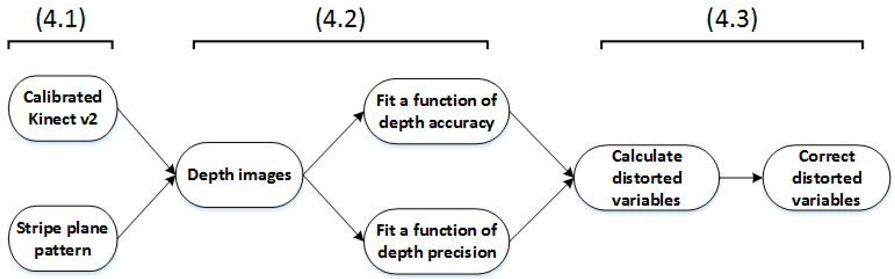
4.1. Calibrate the Kinect v2 and Prepare the Stripe Plane Pattern

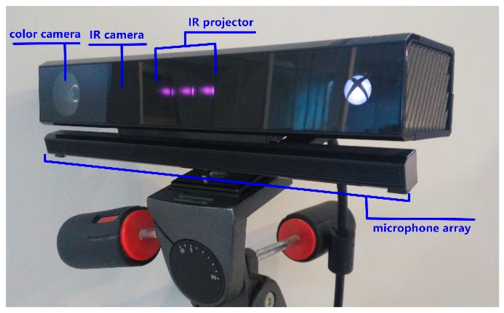
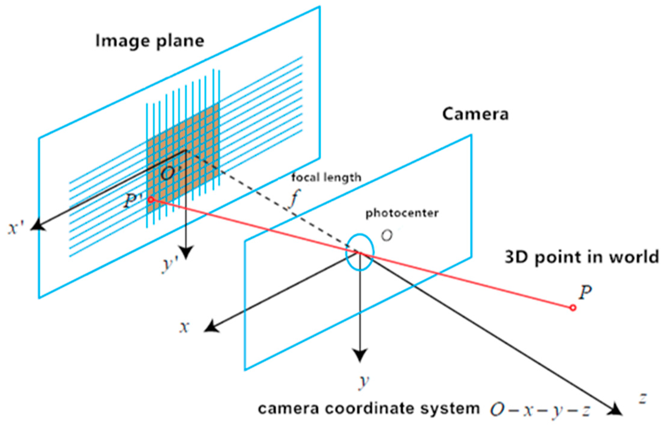
In this paper, we equipped our computer with the Ubuntu 14.04 operating system and libfreenect2 [26], which is the driver for the Kinect v2. Then we printed a chessboard calibration pattern (5 × 7 × 0.03) [18] on A4 paper. Additionally, we used two tripods, one for holding the calibration pattern, and another one for holding the Kinect v2 sensor to calibrate the color, infrared, sync, and depth successively at two distances: 0.9 m and 1.8 m. It is noted that the pinhole camera model is used to explain the corresponding parameters of calibrating the Kinect v2 under different reflectivity.

Actually, there is a possible geo-referencing problem in our post-rectification method. However, in a short distance, the camera can be conducted perfectly orthogonally. Even in the worst condition there is an incidence angle of approximately 8° in its frame edges, which is equivalent to an error of 0.13% for the reflectance value. Therefore, the performance of our proposed algorithm is not affected.

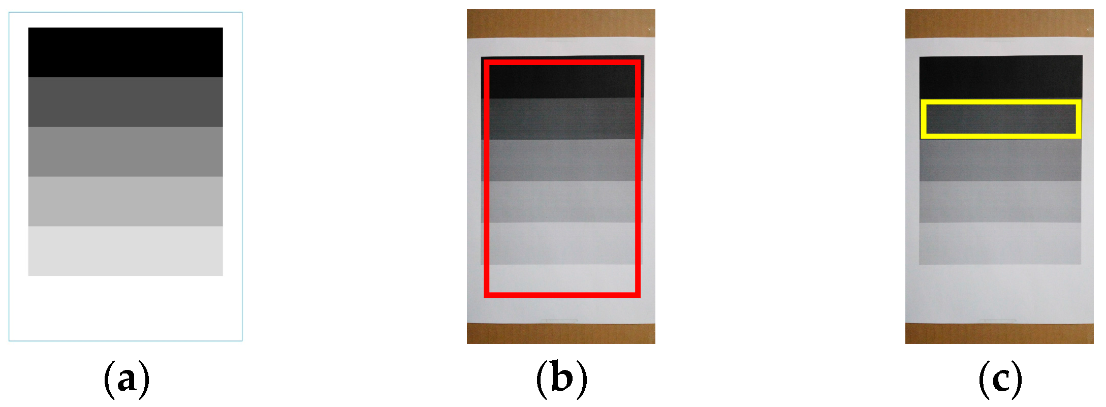
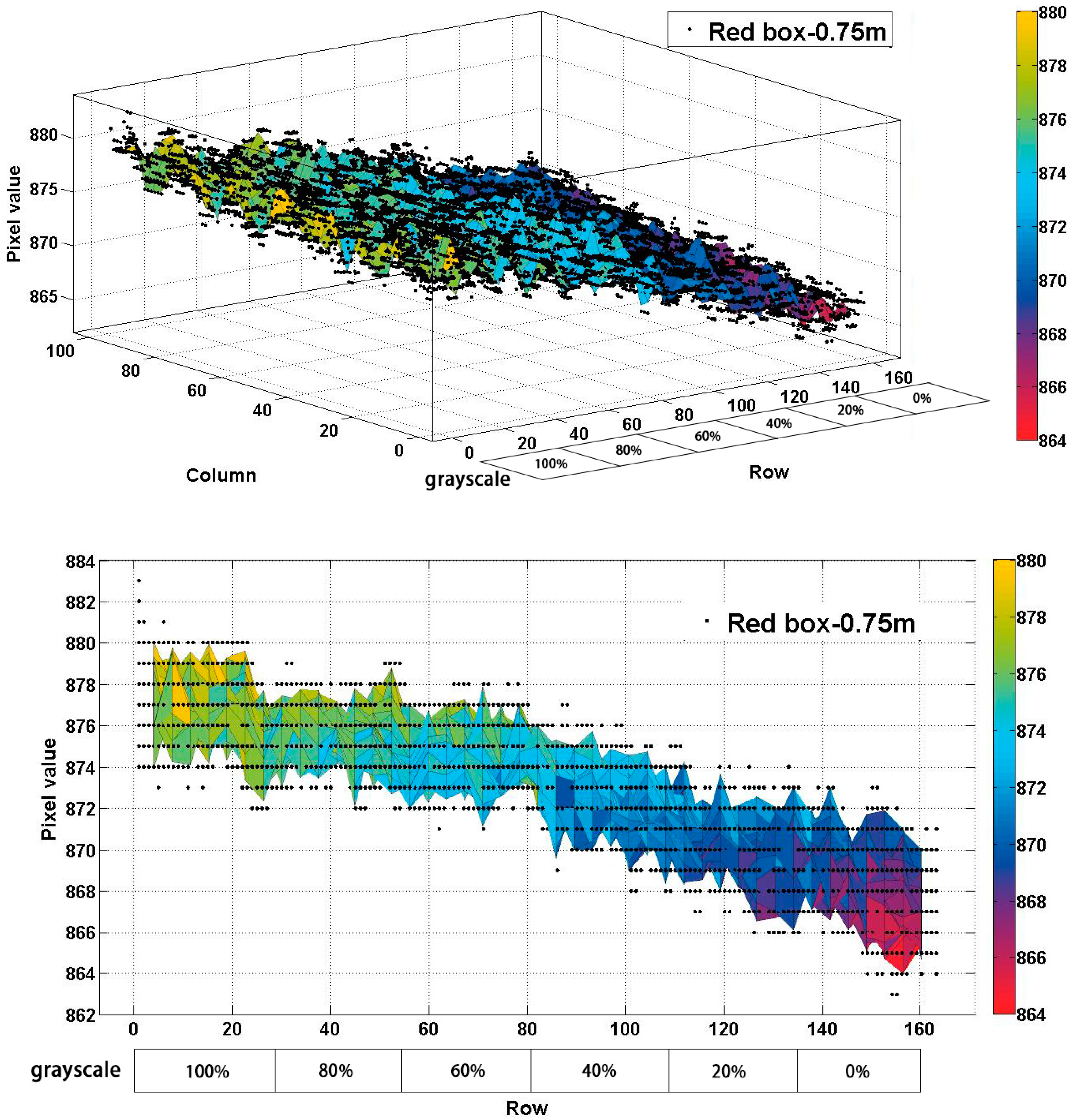
We firstly designed and utilized a stripe plane pattern with different grayscales to investigate the relationship of reflectivity and measured depth. The squared panel divided the gray values into six levels of 100% black, 80% black, 60% black, 40% black, 20% black, and 0% black (white). In the stripe plane pattern, the top strip is printed with 0.0013, decreasing in five steps to 0.9911 (white) from top to bottom with the same size (Figure 4a). This approach is inspired by the Ringelmann card that is usually used in the reflectance calibration. It is noted that the panel is calibrated for wavelengths of 827 nm to 849 nm. These wavelengths are the expected range for the Kinect 2. As we know, the reflectivity is related to the wavelength, so we chose a mean value as the estimated reflectance factor when the wavelength is 838 nm, which is shown in Table 3.

Figure 4. Stripe plane pattern with different grayscales printed on A4 paper: (a) stripe plane pattern on A4 paper; (b) red box region; and (c) yellow box region.

4.2. Capture Depth Images and Fit Functions of Depth Accuracy and Precision, Respectively

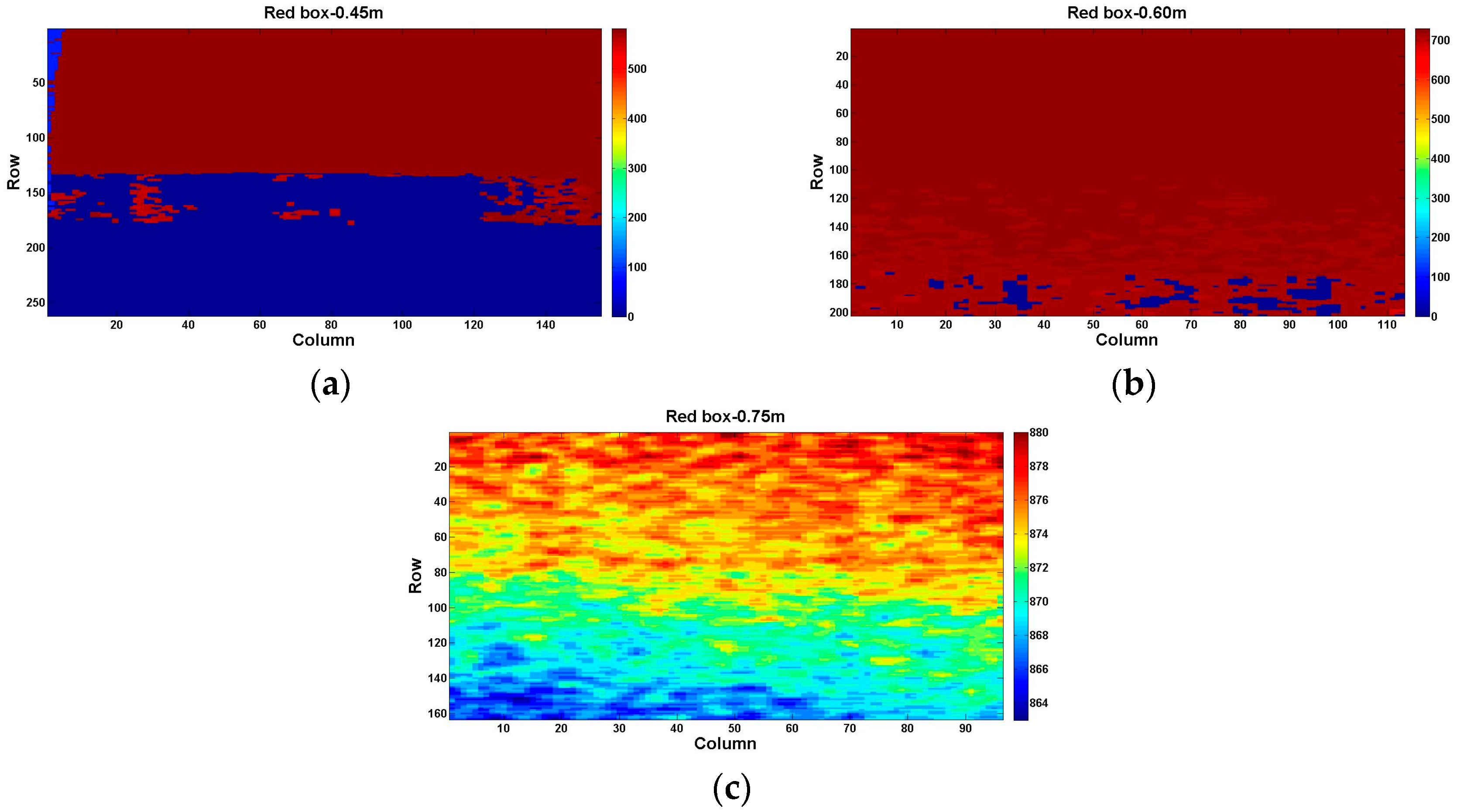
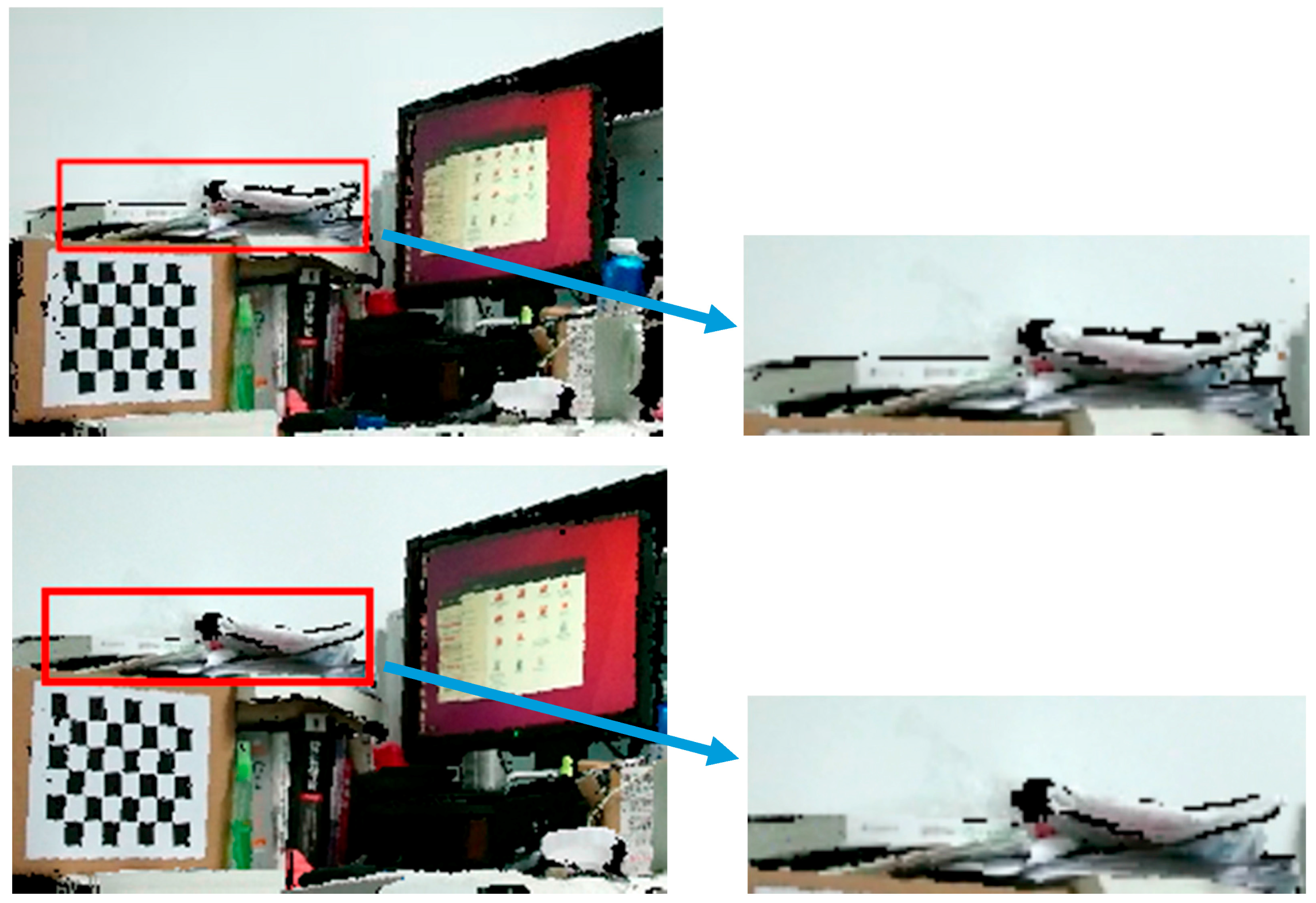
At the same reflectivity, we took the grayscale of 80% black at different distances in the operative measuring range as an example. The region to be studied is presented in Figure 4c with a yellow box.

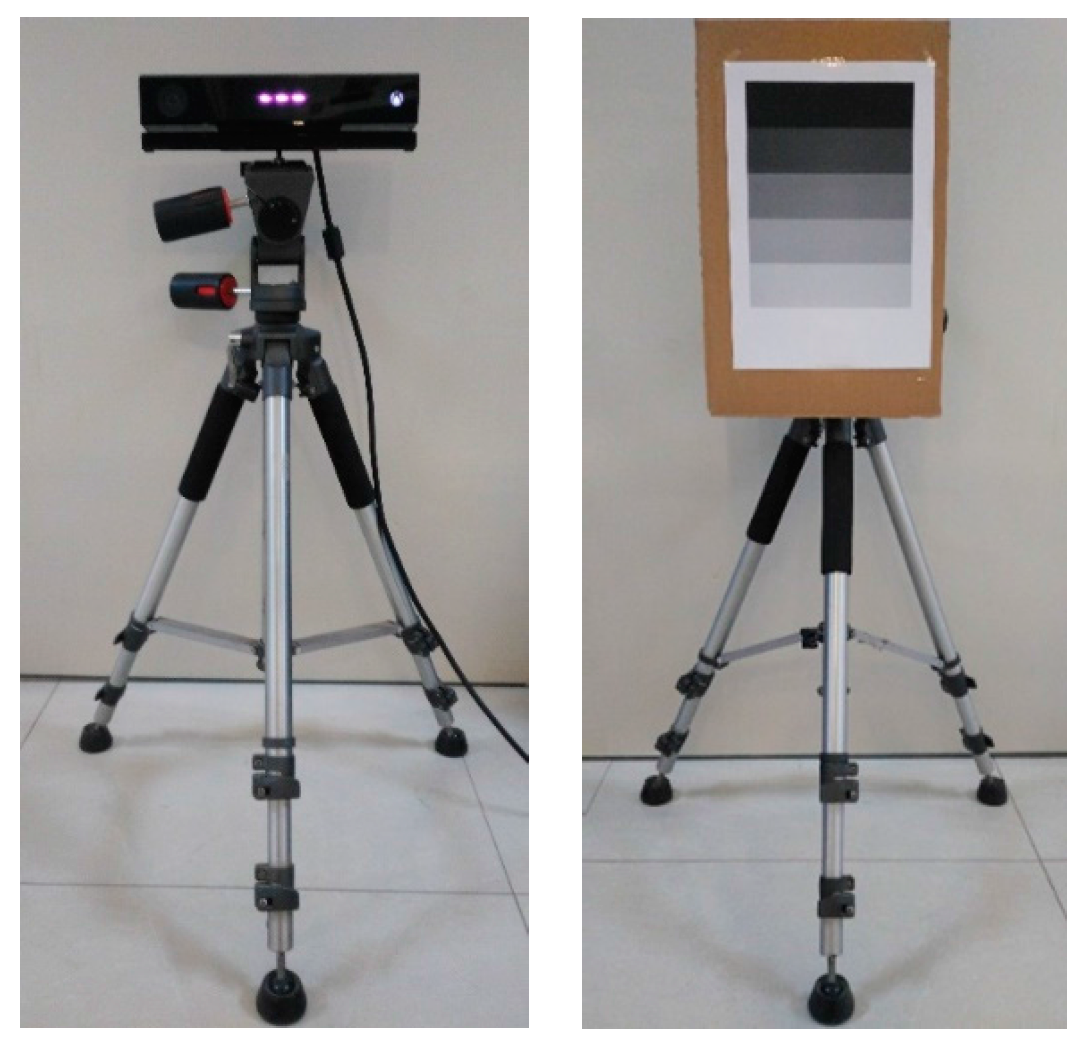
We fixed the calibrated Kinect v2 sensor to a stable tripod, and mounted the stripe plane pattern to the other tripod. As shown in Figure 5, the front panel of the Kinect v2 sensor and the stripe plane pattern are always maintained in parallel, both perpendicular to the ground, using a large triangular rule to guarantee alignment. The stripe plane pattern is progressively moved away from the Kinect v2 sensor in the operative measuring range with a step length of x meters (less than 0.20 m). Therefore, L sets of depth images of the yellow box region are captured. One set contains N (no less than 1) depth images.

Figure 5. Setup of the method: Kinect v2 (left); stripe plane pattern (right).

Step 1: we calculate a mean depth image and an offset matrix of each set of depth images:

$$M_i=\frac{{\displaystyle \sum _{j=1}^N{M}_{ij}}}{N},\left(i=1,2,3,\dots ,L\right)$$

(3)

$$M_{oi}=M_i-M_{gi},\left(i=1,2,3,\dots ,L\right)$$

(4)

where L is the quantity of the depth image sets of the yellow box region captured, i is the sequence number of sets, and N is the quantity of depth images that each set contains, j the sequence number of depth images of each set. M_ij is every depth image of each set, and M_i is the calculated mean depth image of each set. The ground truth matrix is expressed as M_gi (measured by the flexible ruler). Then we obtain an offset matrix M_oi for each distance.

Step 2: we average pixel values of each offset matrix M_oi:

$$m_i=\frac{{\displaystyle \sum _{p=1}^R{\displaystyle \sum _{q=1}^C{m}_{pq}}}}{RC},\left(i=1,2,3,\dots ,L\right)$$

(5)

where R is the number of rows of each yellow box region of each offset matrix M_oi that varies with different distances, p the sequence number of the rows, and C is the number of columns of each yellow box region of each offset matrix M_oi, q the sequence number of the columns. In the offset matrix M_oi, each pixel value offset to the ground truth in the yellow box is represented as m_pq. m_i is the expectation of each offset matrix M_oi.

Step 3: based on Equations (4) and (5), we compute the standard deviation s_i of the offset matrix M_oi for each distance:

$$s_i=\sqrt{\frac{{\displaystyle \sum _{p=1}^R{\displaystyle \sum _{q=1}^C\left(m_{pq}-m_i\right)}}}{RC-1}},\left(i=1,2,3,\dots ,L\right)$$

(6)

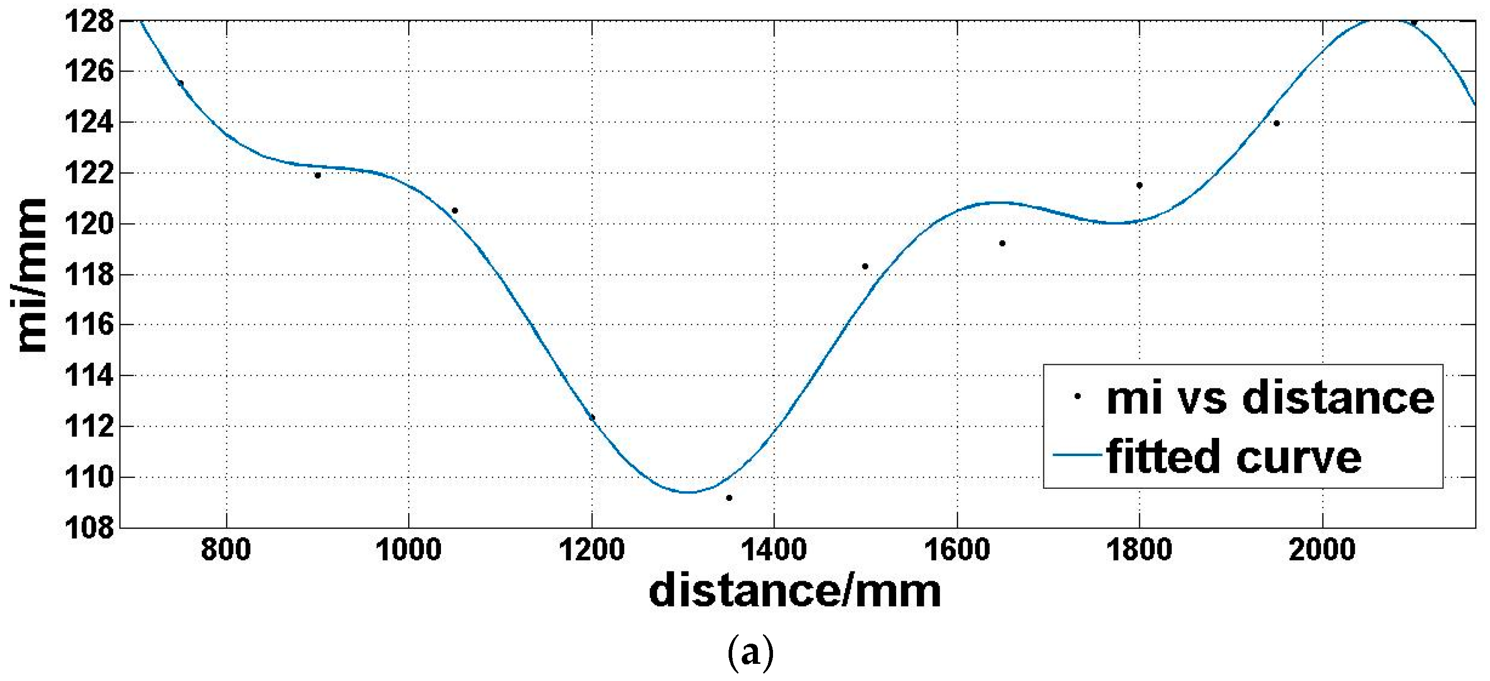
Step 4: we utilize a fitting function three-term sum of sine (Equation (7)) to model the expectation of the offset matrix M_oi (Figure 8a) and a linear polynomial (Equation (8)) to model the standard deviation of the offset matrix M_oi (Figure 8b), which is dependent on the above analysis:

$$m_d=a_1\sin (b_{1}d+c_1)+a_2\sin (b_{2}d+c_2)+a_3\sin (b_{3}d+c_3)$$

(7)

$$s_d=t_{1}d-t_2$$

(8)

where d is the distance, m_d is the offset expectation corresponding to the distance, s_d is the offset standard deviation corresponding to the distance. a₁, a₂, a₃, b₁, b₂, b₃, c₁, c₂, and c₃ are coefficients to be determined in Equation (7). t₁ and t₂ are coefficients to be determined in Equation (8).

4.3. Correct Depth Images

For different distances, we correct the depth image based on Equation (7). The corrected yellow box region depth image is:

$$M_{corr}=M_d-m_d$$

(9)

where M_d is the depth image corresponding to the distance. Then, based on Equations (4)–(6), we can calculate m_corr and s_corr. m_corr represents the corrected expectation of the offset matrix and s_corr represents the standard deviation. 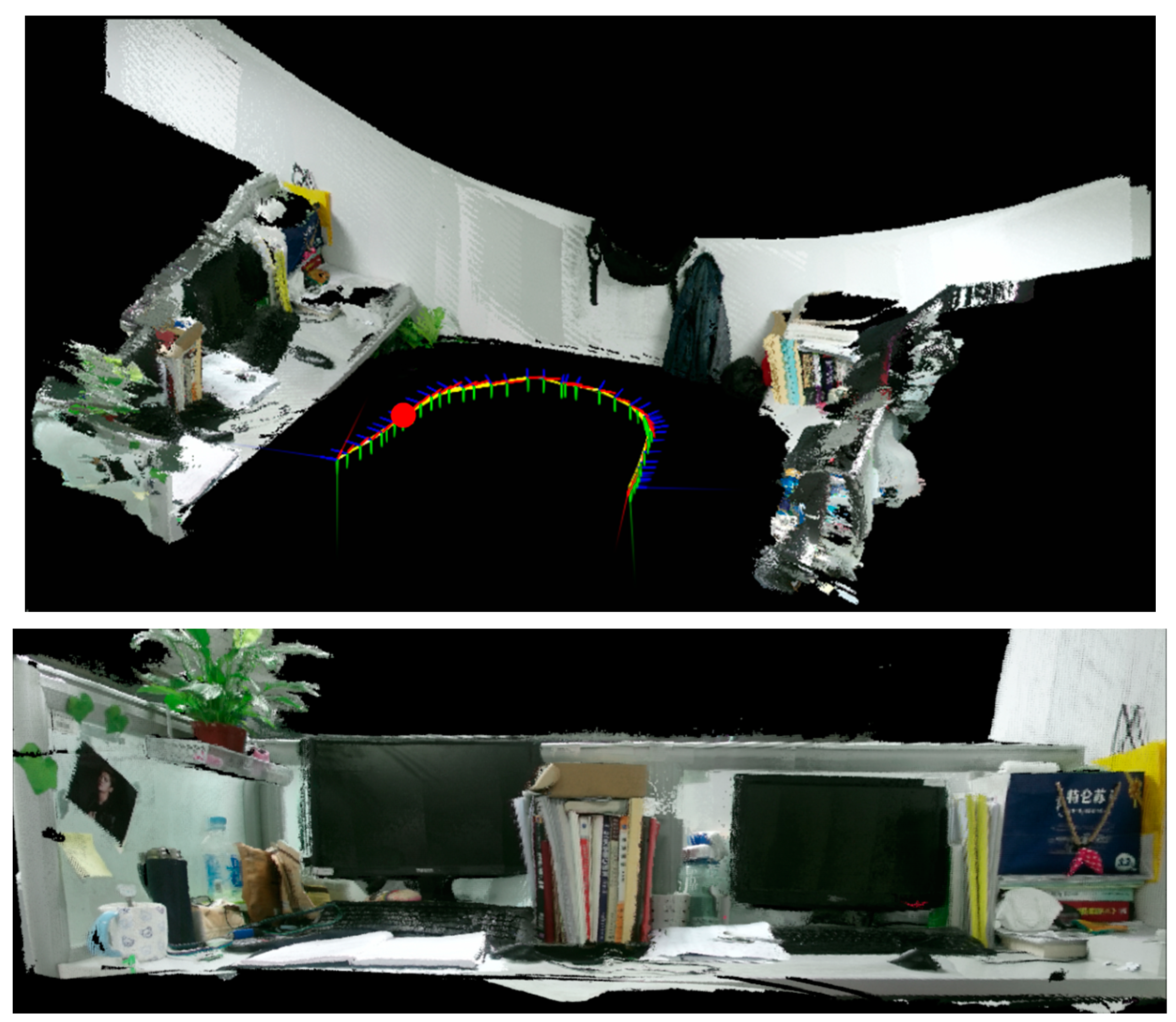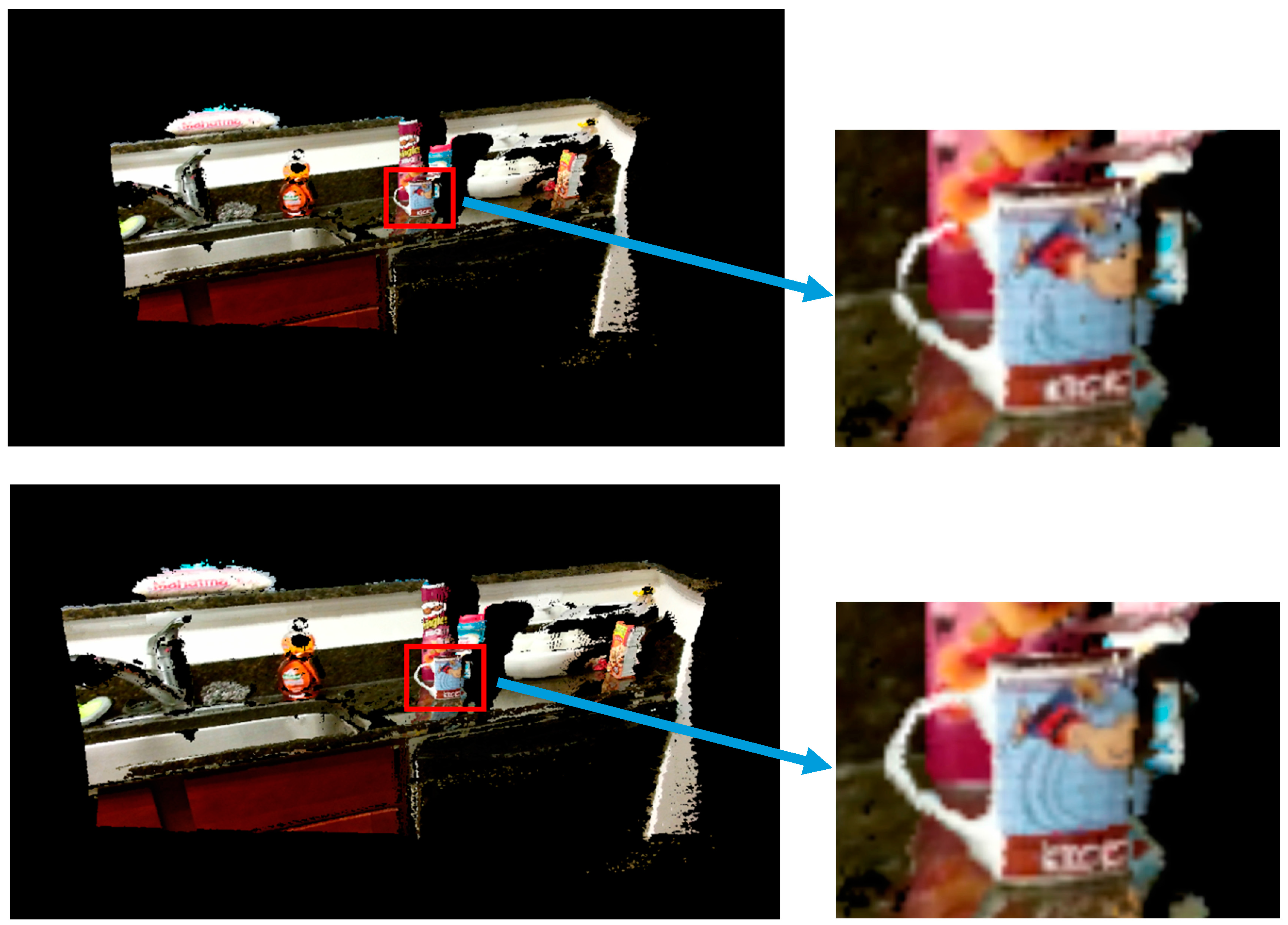The depth accuracy of the Kinect v2 is evaluated by the expectation of an offset matrix of the depth image, and the depth precision is evaluated by the standard deviation [20,22]. In the next section, we apply the post-rectification approach to RGB-D SLAM [6] in an indoor environment to prove its real effect.

5. Experiments and Results

We conducted experiments in an office room with essentially constant ambient background light. It is noted that we spent 40 min to pre-heat the Kinect v2 sensor, for the sake of eliminating the temperature drift effect [13,20].

Since both the accuracy and the precision will decrease with the increasing measuring range [17], and indoor environments are usually small, like our office room environment, the operative measuring range in this paper is no more than 2 m. The tripod with stripe plane pattern is progressively moved away from the Kinect v2 sensor, from 0.45 m to 2.10 m, with a 0.15 m step width. Therefore, 10 sets of depth images of the yellow box region are captured. One set contains five depth images.

We obtain three depth images successively at the first three distance: 0.45 m, 0.60 m, and 0.75 m. By analyzing the same region of the stripe plane pattern (red box in Figure 4b) at these three distances, three visualized depth images of the red box region are illustrated in the Figure 6a–c. It is noted that the color-bar indicates the pixel values of the depth image. We reveal that at a short distance, an invalid null value (pixel value 0) is easy to obtain in high-reflectivity regions at the bottom of the red box, as shown in Figure 6a,b. Summarized, the minimum operative measuring distance is located between 0.60 m and 0.75 m in our indoor environment, which is larger than the official given value of 0.5 m.

Figure 6. Visualized depth images of the red box region at different distances (front view): (a) 0.45 m; (b) 0.60 m; and (c) 0.75 m.

In order to avoid the effect of invalid null value and carry out reliable studies, the distance is adjusted from 0.75 m to 2.10 m, with the same 0.15 m step width in the following experiments.

5.1. Same Distance, but Different Reflectivity

At the same distance, six kinds of different reflectivity in the red box on the stripe plane pattern (Figure 4b) affect the measured distance obviously. As shown in the top of Figure 7, with the reflectivity increases (row axis from small to large in Figure 7, or rows of the red box, top to bottom in Figure 4b), the measured distance becomes smaller at a distance of 0.75 m. Figure 6c also illustrates the fact for a distance of 0.75 m in the front view. Furthermore, it is presented clearly in the side view at a distance of 0.75 m in the bottom of Figure 7.

Figure 7. Red box region at distance 0.75 m: 3D view (top); side view (bottom).

5.2. Same Reflectivity, but Different Distances

Based on Section 4, we carry out experiments with the post-rectification approach to investigate the relationship between the measured depth and six kinds of reflectivity on the stripe plane pattern (Figure 8), respectively. The experimental results are shown in Table 4, where m_corr is the standard deviation of the depth information difference between the corrected and the ground-truth, S_corr is the expectation of m_corr, m is the standard deviation of the depth information difference between the un-corrected values and the ground-truth, and s is the expectation of m. It should be noted that m is achieved by using the post-rectification that was proposed by [23].

Figure 8. Expectation (a) and standard deviation (b) of offset matrix M_oi under the same reflectivity and different distances.

Table 4. Expectation and standard deviation of correction and uncorrection at different reflectivity.

		Distance (m)	0.75	0.90	1.05	1.20	1.35	1.50	1.65	1.80	1.95	2.10
	Value (mm)
Item
100% black
mcorr			0.1607	−0.4710	0.6894	−0.2793	−0.5033	1.0029	−1.5421	1.1476	−0.7082	−0.0217
Scorr			2.0669	2.3116	2.4457	2.4295	3.2557	3.1760	3.9849	3.6780	5.1154	4.4273
m			127.6166	123.7936	122.8260	114.3370	111.3207	119.5455	121.4907	123.1732	124.5892	129.7157
s			2.0669	2.3116	2.4457	2.4295	3.2557	3.1760	3.9849	3.6780	5.1154	4.4273
80% black
mcorr			0.0873	−0.3563	0.4352	−0.0085	−0.7791	1.2867	−1.5841	1.4674	−0.6622	0.2705
Scorr			1.0963	1.3948	1.3684	1.5997	1.9776	2.3625	2.1146	1.8148	2.0750	3.4419
m			125.5293	121.8862	120.5257	112.3133	109.1780	118.3241	119.2202	121.5227	123.9722	127.9327
s			1.0963	1.3948	1.3684	1.5997	1.9776	2.3625	2.1146	1.8148	2.0750	3.4419
60% black
mcorr			0.3129	−0.6364	1.1514	−0.6131	−0.3607	1.0400	−1.9007	1.4719	−1.0410	−0.0744
Scorr			1.2006	1.3411	1.4766	1.1424	1.4639	1.7628	1.9563	1.6953	1.7913	2.2094
m			124.6040	121.4815	120.6797	111.3145	109.1095	116.9787	118.4527	121.9892	123.6846	128.0617
s			1.2006	1.3411	1.4766	1.1424	1.4639	1.7628	1.9563	1.6953	1.7913	2.2094
40% black
mcorr			0.0478	−0.0596	0.1218	0.0904	−0.4571	0.6311	−0.8309	0.6094	−0.4894	−0.0280
Scorr			1.4408	1.7909	1.4628	1.4888	1.2835	1.5967	1.2283	1.3882	2.8126	1.6514
m			122.3192	120.1545	117.1464	109.2976	107.1321	114.7480	116.7984	119.2528	123.7405	125.8464
s			1.4408	1.7909	1.4628	1.4888	1.2835	1.5967	1.2283	1.3882	2.8126	1.6514
20% black
mcorr			0.1038	−0.7496	0.9256	−0.5031	−0.2778	1.0179	−1.3685	1.6489	−0.4917	0.4327
Scorr			1.3713	1.6607	1.6392	1.4375	1.5381	1.8762	1.4057	1.2839	1.4366	2.5210
m			120.0186	116.1750	116.2189	108.1833	106.1495	113.9487	115.8037	118.9490	121.4179	125.7333
s			1.3713	1.6607	1.6392	1.4375	1.5381	1.8762	1.4057	1.2839	1.4366	2.5210
0% black (100% white)
mcorr			0.6980	0.0054	1.3	0.3592	−0.0831	1.8191	−1.0919	2.2539	−0.2420	0.7992
Scorr			1.6839	1.8881	1.7393	1.6467	1.7178	2.0895	1.3940	1.1620	1.4396	2.6236
m			117.5105	113.7644	113.7520	105.6693	103.2963	112.9783	114.3643	117.4583	120.2713	124.4468
s			1.6839	1.8881	1.7393	1.6467	1.7178	2.0895	1.3940	1.1620	1.4396	2.6236

It is noted that in a short distance, the camera can be conducted perfectly orthogonal. Even in the worst condition, an incidence angle approximately 8° in its frame edges, which is equivalent to an error of 0.13% for the reflectance value. Therefore, the performance of our proposed algorithm is not affected.

As bold data show in Table 4, for the depth accuracy, we obtain the best experimental results below 1 mm at a grayscale of 40% from a distance 0.75 m to 2.10 m. Correspondingly, at a high reflectivity at a grayscale of 0%, the depth accuracy is below 3 mm, which is the whole depth accuracy. It is noted that our accuracy is better than the result (its accuracy is 5 mm) which is indicated in [22]. Moreover, the experimental results in [22] were achieved by a classic rectification measurement. Furthermore, for the depth precision, we obtain the best experimental results below 3 mm at a grayscale of 60% from a distance 0.75 m to 2.10 m. At a low reflectivity at a grayscale of 100%, the depth precision is below 6 mm, which is the whole depth precision.

Furthermore, after analyzing Figure 7b and Table 4, we can indicate that our proposed post-rectification algorithm is a linear model, as we stated in the previous section. This is because S_corr is the same with s.

There are two possible explanations for intensity-related effect for Kinect v2. One assumption is a specific variant of a multi-path effect, and the other one puts this effect down to the nonlinear pixel response for low amounts of incident intensity.

Finally, following the instructions proposed in Section 4.2, we complete the calibration of the Kinect v2 and acquire a series of parameters that the Kinect v2 needs in Table 5.

Table 5. Parameters from the calibration of the Kinect v2 (by rounding).

Camera	Intrinsic Parameters
	fx (mm)	fy (mm)	u0 (pixel)	v0 (pixel)
Color	1144.361	1147.337	966.359	548.038
IR	388.198	389.033	253.270	213.934
Camera	Distortion Coefficients
	k1	k2	k3	p1	p2
Color	0.108	−0.125	0.062	−0.001	−0.003
IR	0.126	−0.329	0.111	−0.001	−0.002
	DepthShift (mm)
IR	60.358
	Rotation Matrix		Translation Vector
Color and IR	$\left[\begin{array}{ccc}0.99997& 0.00715& -0.00105\\ -0.00715& 0.99995& 0.00662\\ 0.00110& -0.00661& 0.99998\end{array}\right]$		${\left[-0.06015,0.00221,0.02714\right]}^{\mathrm{T}}$

5.3. Application for RGB-D SLAM System

In the sake of proving the effect of the post-rectification approach, we apply it to RGB-D SLAM [6] in an indoor environment. Our indoor scene under experiment is around 1.4 m away from the Kinect sensor, so we calculate the expectation of offset of six kinds of reflectivity according to Section 4 at a distance 1.4 m. The results are shown in Table 6.

Table 6. The expectation of offset of six kinds of reflectivity at distance 1.4 m.

	Reflectivity	0.9913	0.7981	0.6019	0.4125	0.1994	0.0011
Expectation (mm)
m		107.3987	109.0536	109.8727	112.3605	113.0718	115.2330

As shown in Table 6, with the decrease of reflectivity (an increase of the grayscale level), the expectation of offset is progressively rising. Then we average those six values of expectation to be the deviation of this indoor scene. After correction, an average of 118 mm deviation is eliminated. Via the offline RGB-D SLAM method, Figure 9 presents two kinds of point clouds magnified by the same multiples before and after correction by using our proposed method. Therefore, it is obvious that, after correction, the scene is closer to the Kinect v2 sensor than before in the point cloud, which indicates that the depth accuracy of the point cloud is improved. Moreover, an excellent visual effect point cloud of this indoor scene is displayed in Figure 10. The line in the middle of the top overall view is the trajectory of Kinect v2. The bottom is a side view at the red point position of the trajectory in the top overall view.

Figure 9. Point cloud of an indoor scene before (top) and after (bottom) correction using the post-rectification approach.

Figure 10. Point cloud of this indoor scene: overall view (top); a side view at the red point position in the overall view (bottom).

Furthermore, we apply the post rectification approach to the George Mason University (GMU) Kitchen Dataset [27], which is captured by a Kinect v2. Figure 11 shows the point cloud before and after correction by using our proposed method. According to the two red rectangles of Figure 11, we can find that the bottle is larger after using our post-rectification, while losing little information, which can support more useful scene information than without post-rectification. This is due to using precision depth data.

Figure 11. A point cloud of the GMU Kitchen Dataset before (top) and after (bottom) correction using the post-rectification approach.

6. Conclusions

Within this work, we analyze the relationship between the measured distance of the depth image and reflectivity of the indoor scene for the Kinect v2 depth sensor in detail. Based on the analysis of reflectivity-related depth error, this paper proposes a post-rectification methodology to correct the depth images. We utilize a calibrated Kinect v2 and a stripe plane pattern to capture depth images of the indoor environment. Then, the functions of depth accuracy and precision are fitted respectively with the depth images. Finally, according to the fitting functions, we can correct the dataset’s depth images to obtain more accurate and precise depth images so as to generate a point cloud. As the experimental results show, the accuracy is below 3 mm from a distance of 0.75 m to 2.10 m, which is 2 mm lower than that in [22]. Moreover, the precision is below 6 mm, which is 2 mm lower than that in [22]. Therefore, our proposed post-rectification approach outperforms the previous work, which will be useful for high-precision 3D mapping of the indoor environments, as well as subsequent semantic segmentation and semantic understanding.

Further studies will consider applying the post rectification approach to 3D reconstruction of indoor scenes in real-time with the Kinect v2 sensor.