1. Introduction
Landslides, as geological hazards causing serious casualties, property loss, and environmental damage, restrict sustainable development [
1,
2]. To minimize economic losses and loss of human life, landslide-prone areas should be identified. A landslide susceptibility map is urgently needed.
Numerous models and approaches for landslide susceptibility mapping have been developed throughout the world over the past decades [
3,
4,
5,
6,
7]. The most used methods are based on soft computing or statistical techniques, e.g., the fuzzy logic method [
8,
9], artificial neural network model [
10,
11], logistic regression model [
12,
13], cellular automata methods [
14], and analytic hierarchy process [
15,
16].
The information value based method has been widely applied as a statistical data-driven method recommended by experts [
17] to assess landslide susceptibility [
18,
19]. Xu et al. [
18] used GIS and the information value model to evaluate debris flow susceptibility. Chen et al. [
19] made a landslide susceptibility map using the information value model in the Chencang District of Baoji, China. Zhu et al. [
20] compared the information value model with the weights-of-evidence method in landslide susceptibility mapping. The results demonstrate that the information value model had higher prediction accuracy. Chen et al. [
21] made a comparison between the information value model and logistic regression model in landslide susceptibility mapping, which suggests that the results of the information value model were more coincident with actual landslide events. The higher prediction accuracy of the information value model in landslide susceptibility mapping is partly because the relative weights of different classes of each landslide predisposing factor can be determined objectively. In addition, different factors have different influences on the occurrence of landslides. However, the traditional information value model regards all landslide predisposing factors at the same level of importance and assigns equal weight to each factor. Thus, this model cannot reflect the differences between the contributions of various landslide predisposing factors. To improve the information value model, several methods have been proposed. Jiang et al. [
22] combined the information value model with an analytic hierarchy process to assess landslide susceptibility. An information value model integrated with Shannon’s entropy was proposed by Sharma et al. [
23]. However, for these methods, the weights of landslide predisposing factors are determined through human intervention, which increases uncertainties in the results.
This paper proposes an improved information value model based on gray clustering. Since the effects of various predisposing factors on landsliding are different. It is vital to understand the differences in effect and hence to weight the importance of different factors. This model objectively determines both the relative weights of different classes within each predisposing factor and the weights of predisposing factors for landslides. The proposed model is evaluated by comparing its landslide susceptibility mapping results with those of the traditional information model and the improved model combined with the analytic hierarchy process. This study provides new insight for landslide susceptibility mapping that can help governments to conduct landslide prevention and mitigation.
2. Study Area
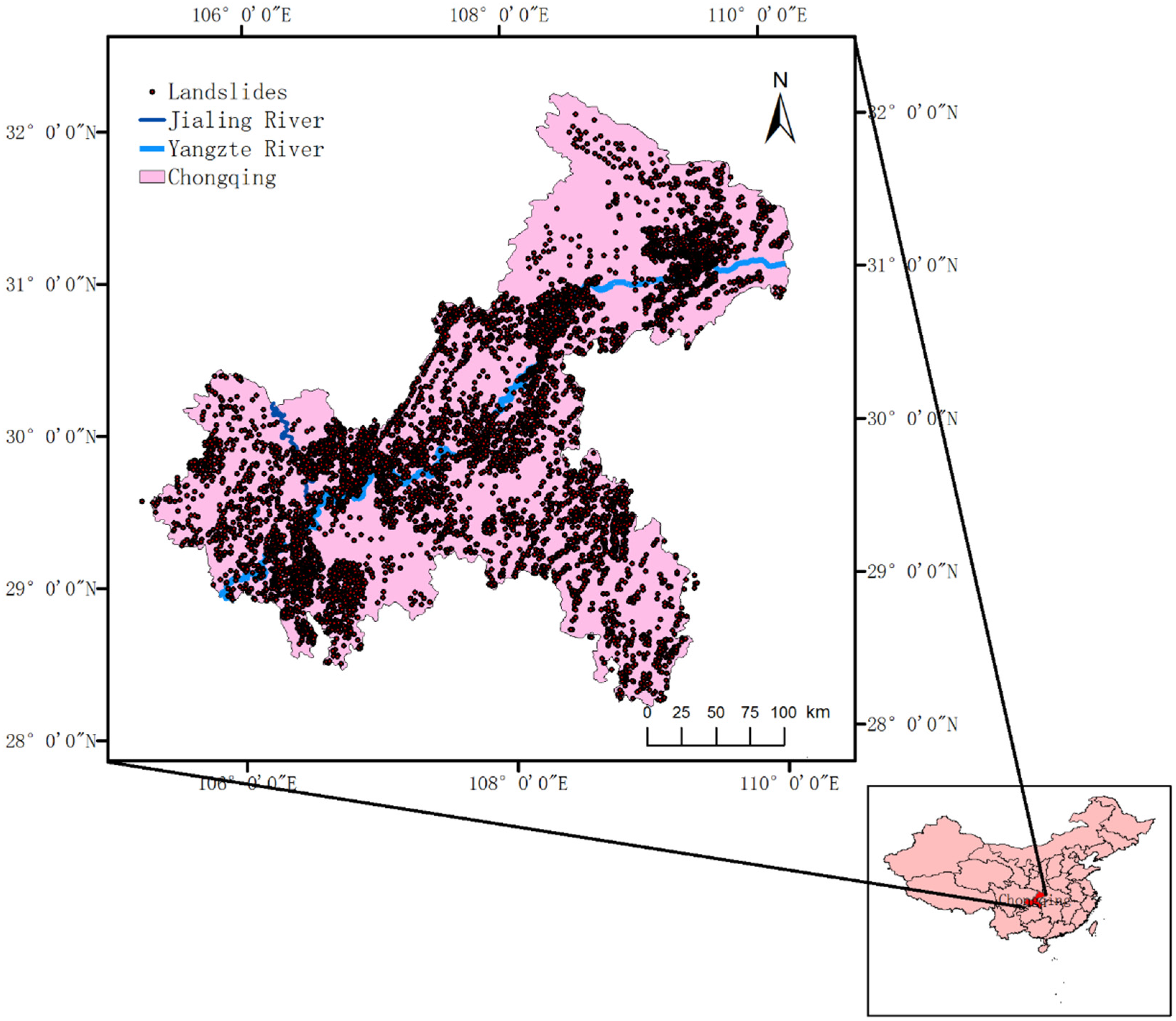
The study area of Chongqing is located in the southwestern part of China, between the longitudes 105°11′ E and 110°11′ E and latitudes 28°10′ N and 32°13′ N. This area is characterized by a complex geological structure, soft surface layer, deep valleys, and steep slopes. The basic tectonic framework of this area originated from Indosinian—Yanshan movement and Himalayan movement. Affected by the Huayingshan fault zone, Qiyaoshan fault zone, and Changshou—Zunyi fault, a series of tectonic folds and faults developed in this area. Chongqing is located in the eastern part of Sichuan Basin. The eastern Chongqing is connected to the Qinba Mountains and Wuling Mountains, and the Western Chongqing is linked with the Mid-Sichuan Hilly Region. This area has a distinct topographical relief that is controlled by geological structures. The mountain alignment is broadly consistent with the tectonic line. West Chongqing has mainly low mountainous and hilly regions. The Jialing River and Yangtze River run through the whole region. The climate of this area is subtropical monsoonal, with abundant precipitation and storms. In recent years, increasing human activities in this region, especially for the construction of the Three Gorges Reservoir, caused more impact on the natural terrain. Consequently, landslides became the most extensive and serious geological hazard in the area.
3. Data
3.1. Landslide Inventory Data
In this study, a landslide inventory with a total of 8435 landslide events before 2014 was provided by the Chongqing Institute of Geology and Mineral Resources (
Figure 1). All landslide events are represented by point features with attributes of latitude, longitude, and area. The minimum area of landslides was 3 m
2, and the maximum area was 3,080,000 m
2.
Landslides in the inventory are mainly distributed along the faults, road network, and hydrographic network. The inventory is composed of rotational slides, translational slides, and debris flows and so on. These landslides affect a total area of 194,442,814 m2. According to the landslide volume, these landslides can be divided into four classes, including small-sized landslides (<10 × 104 m3), medium-sized landslides (10 × 104–100 × 104 m3), large-sized landslides (100 × 104–1000 × 104 m3), and huge-sized landslides (>1000 × 104 m3). The number of small-sized landslides, medium-sized landslides, large-sized landslides, and huge-sized landslides is 7052, 1172, 160, and 51, respectively. Landslide disasters in Chongqing are dominated by small-sized landslides (83.6%), followed by medium-sized landslides (13.9%). Large-sized and huge-sized landslides are extremely rare.
The main predisposing factors of landslides in Chongqing include rainfall, earthquakes, erosion of slope toes by rivers, and human activities. Most landslides in the study area are caused by rainfall, followed by landslides caused by earthquakes and erosion. Some studies have indicated that the rainfall threshold was 150 mm/day in the study area [
24]. Moreover, a great number of construction projects initiated by local governments were also responsible for the landslide occurrence.
3.2. Landslide Predisposing Factors
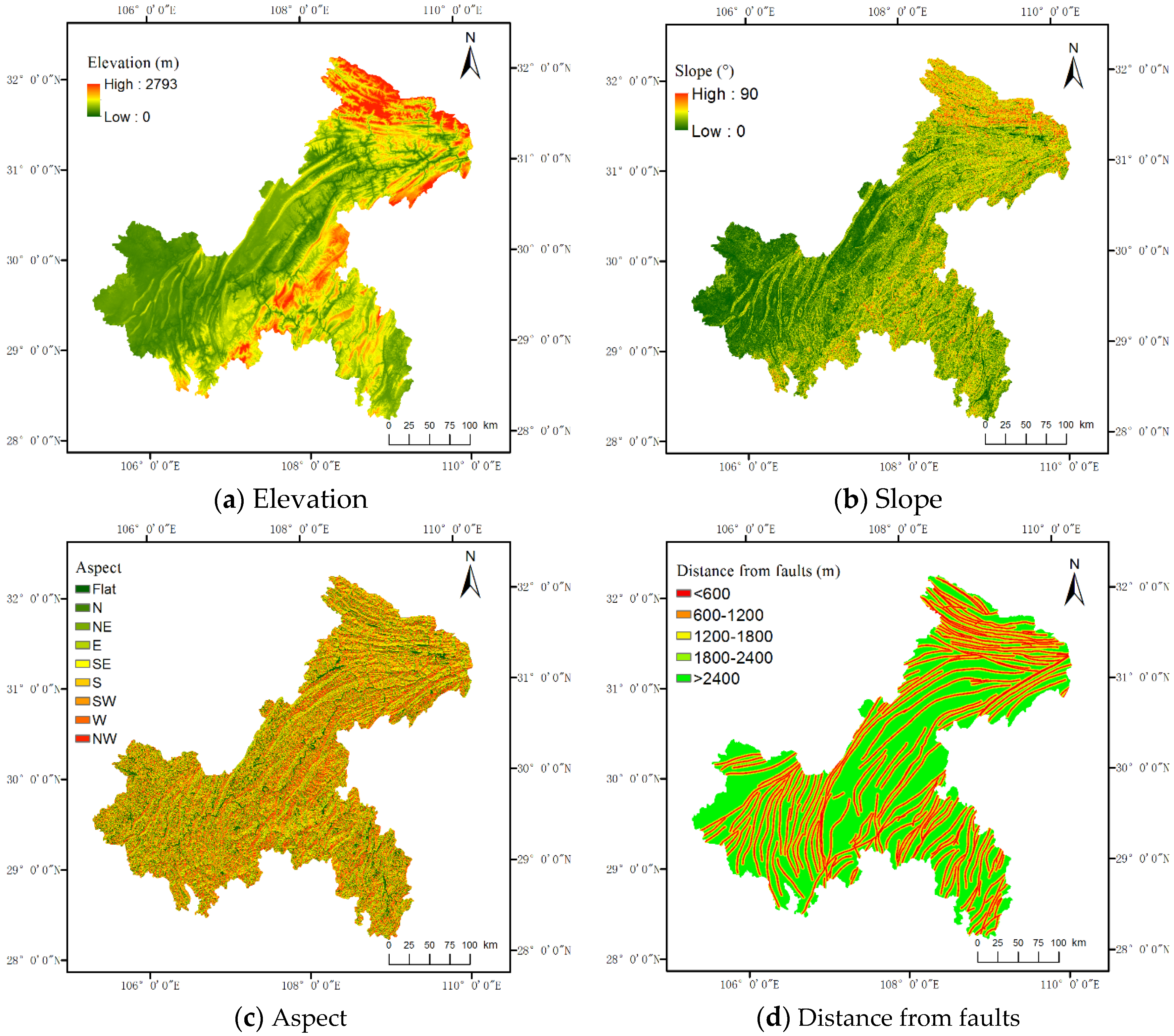
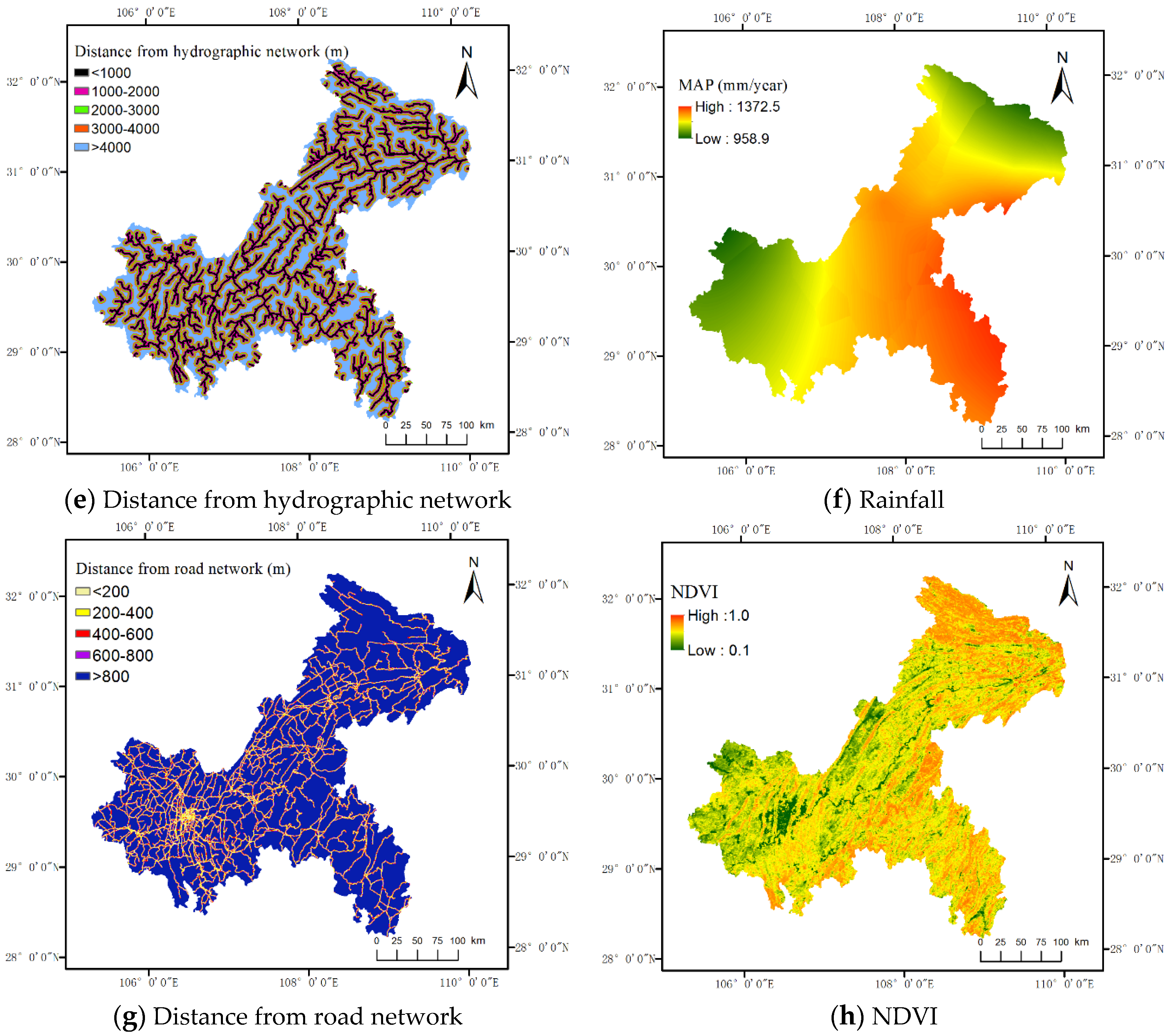
In this paper, we utilized eight landslide predisposing factors to construct landslide prediction methods, including elevation, slope gradient, aspect, rainfall, distance from the faults, distance from the road network, distance from the hydrographic network, and the normalized difference vegetation index (NDVI).
Elevation has great effects on climate, hydrology, geology, and soil, which are factors related to the occurrence of landslides. Slope gradient is a main driving force of landsliding. Theoretically, landslides are more likely to occur on steep slopes [
25]. However, some studies have reported that landslides are most likely to occur when the slope gradient is moderate [
26]. This is due to a lack of material foundation for landsliding at large slope gradients [
27]. Aspect influences the distribution of water and heat resources and, hence, affects soil, rock, and vegetation types [
28]. Rainfall is an important triggering factor of landslides by directly or indirectly reducing the shear strength of rock-soil through physical and chemical effects on rock-soil. Therefore, the mean annual precipitation (MAP) is used as the indicator. Proximity of a fault is also a main predisposing factor for landslides. It is well known that landslides tend to occur in the surrounding area of a fault due to fractures in the rock mass [
29,
30]. The buffer distance from the faults is used as the indicator. Road construction also results in the oversteepening of side slopes. Therefore, there is a high probability of landslide occurrence along a road. The distance of a slope to drainage structures is another important factor for slope stability. Streams may adversely affect stability by eroding the slopes or saturating the lower part of material [
31,
32]. Therefore, we chose the distance from the hydrographic networks as a predisposing factor. NDVI is an important index denoting a region’s vegetation cover, and it is an important factor for landslide occurrence and movement [
33]. Plant roots can hold the soil to mitigate the effect of rainfall [
34]. Theoretically, the possibility of landslide occurrence gradually decreases with increasing NDVI value [
35].
The 30-m-resolution global digital elevation model generated from the stereoscopic data collected by the advanced spaceborne thermal emission and reflection radiometer global digital elevation model (ASTER GDEM) was utilized to provide elevation information. Based on ASTER GDEM, a slope gradient and an aspect map were generated. The hydrographic network was also extracted from ASTER GDEM by computing flow accumulation. The geological structure data extracted from a geological map of Chongqing was in vector format on a scale of 1:500,000. The road network vector data was retrieved from the topographic map of China. The rainfall data, including daily precipitation at rainfall observation stations in 2013 and 2014 and geographical coordinates of these observation stations, was provided by the Chongqing Institute of Geology and mineral resources. The NDVI data were provided by International Scientific & Technical Data Mirror Site, Computer Network Information Center, Chinese Academy of Sciences. (
http://www.gscloud.cn) at a resolution of 500 m and resampled to a resolution of 30 m. Landslide predisposing factors maps are shown in
Figure 2.
4. Methodology
For the data set, each 30 × 30 m grid cell was used as the study unit. The 8435 recorded landslides were randomly divided into two subsets. The 70% (5905) of inventory landslides were used for model training, and the remaining 30% (2530) were used for model validation. The three models, i.e., the information value model, the improved information value model based on analytic hierarchy process and the improved information value model based on gray clustering, were used to assess landslide susceptibility. Finally, landslide susceptibility was divided into the following five classes: very low, low, moderate, high, and very high using Jenks natural breaks optimization. Jenks natural breaks optimization is a data clustering method designed to determine the best arrangement of values into different classes. This is done by seeking to minimize each class’ average deviation from the class mean, while maximizing each class’ deviation from the means of other groups. In other words, the method seeks to reduce the variance within classes and maximize the variance between classes [
34]. Details of the three models are provided in the following subsections.
4.1. Information Value Model (IVM)
IVM is a statistical analysis method that was developed from information theory. In this model, information values of predisposing factors were used to characterize the possibility of landslides occurrence. The information value
of each landslide predisposing factor
can be expressed as follows [
21,
36,
37]:
where
represents the likelihood of landsliding,
is the total number of study units from the study area,
is the total area of landslides in the study area which is the sum of area of all landslide points in the study area,
is the number of the study units with the presence of predisposing factor
, and
is the total area of landslides with the presence of predisposing factor
which is the sum of area of the landslide points with the presence of predisposing factor
.
Therefore, the total information
of each study unit can be calculated as the sum of the information values of all predisposing factors [
38].
when
, the possibility of landslide occurrence is lower than average; when
, the possibility of landsliding is equal to average; and when
, the possibility of landsliding is higher than average [
39]. The larger the information value, the greater the possibility of landsliding.
The method is composed of the following steps: (1) Preprocessing landslide data and landslide predisposing factors data. Generating the slope and aspect distribution map by the use of DEM data and hydrology tool of ArcGIS. Thorough buffer area analysis of hydrographic network, road network, and faults generating the corresponding buffer maps. The rainfall should be interpolated to draw the rainfall distribution map; (2) Classifying landslide predisposing factors, then calculating information values of landslide predisposing factors according to Equation (1); (3) Overlaying the information values distribution maps of all landslide predisposing factors to calculate total information by the use of the map algebra tool, ArcGIS; and (4) Reclassifying the total information using Jenks natural breaks optimization to generate a landslide susceptibility map.
4.2. The Improved Information Value Model Based on Analytic Hierarchy Process (IVM-AHP)
IVM can be improved using an analytic hierarchy process. The construction of the improved model consists of the following steps [
15,
40,
41,
42]:
- 1
For the establishment of the hierarchy, with 1–9 and its reciprocal as the scale of the importance of predisposing factors on landslide occurrence (
Table 1), the relative importance of predisposing factors is compared to construct a pairwise comparison matrix [
43].
- 2
The largest eigenvalue and corresponding eigenvector of the comparison matrix are calculated. The eigenvector is normalized to represent the weights of predisposing factors [
44,
45,
46].
- 3
The consistency of the matrix is checked. Consistency ratio
is used to calculate the consistency as Equation (3)
where
is the mean random index that has been defined by Saaty [
47] (
Table 2).
is the consistency index that is defined as
where
is the largest eigenvalue and
is the order of the comparison matrix. When the value of
is less than 0.1, the pairwise comparison satisfies the consistency requirements [
48,
49]. Otherwise, the comparison matrix must be reconstructed, which means that we should return to the first step [
50].
- 4
The total weighted information value of each study unit is obtained using the information values derived from the IVM according to Equation (5):
In this equation,
is the weight of each predisposing factor. Then, the total weighted information value can be reclassified using Jenks natural breaks optimization to generate the landslide susceptibility map.
4.3. The Improved Information Value Model Based on Gray Clustering (IVM-GC)
In this paper, the model (IVM) described in
Section 4.1 is improved based on gray clustering. The information value derived from the IVM is used to obtain the relative weights of different classes within each landslide predisposing factor and to determine the weights of these factors.
In landslide susceptibility mapping, study units are clustering objects that are denoted by
and landslide predisposing factors as clustering indexes are expressed as
. The value of the
th predisposing factor at the
th study unit is expressed as
. Gray classes
are regarded as landslide susceptibility classes. The
is the total number of study units. The
is the number of landslide predisposing factors, which is 8 for this paper. The
is the number of landslide susceptibility classes, which is 5 in this study. Gray clustering for the landslide susceptibility mapping has the following steps [
51,
52,
53]:
- 1
Using a min-max normalization method, the data are normalized to eliminate the influence of dimension. Among all
values, the maximum value
and the minimum value
are used to normalize
[
52]:
- 2
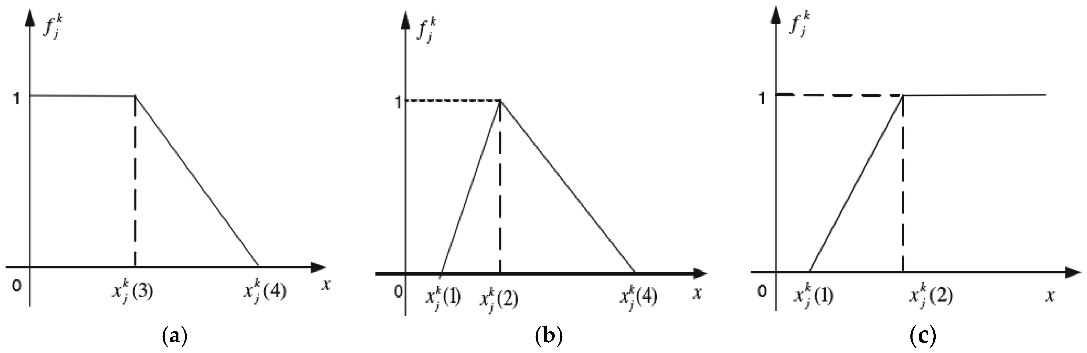
The whitening weight functions of predisposing factors are determined. The
is the whitening weight function of the
th susceptibility class of the
th predisposing factor [
52].
- ①
The lower whitenization weight function (
Figure 3a) is
- ②
The moderate whitenization weight function (
Figure 3b) is
- ③
The upper whitenization weight function (
Figure 3c) is
- 3
The clustering weight
which reflects the influence of each landslide predisposing factor on landslide occurrence, is calculated by Equation (10):
where
is the sum of the positive information values of the
th landslide predisposing factor. The
is the total positive information value of all predisposing factors.
- 4
The clustering coefficient of the study unit
for the susceptibility class
is expressed as
where
is the clustering weight functions in step (2), and
is the normalized value of the
th predisposing factor at the
th study unit. The clustering weight
is obtained in step (3).
All the clustering coefficients of the
th study unit constitute a clustering vector:
- 5
According to the clustering vector, the susceptibility class that the study unit
belongs to can be determined. The study unit
belongs to the class
if
i.e.,
equals the value of
whose clustering coefficient
is the largest.
4.4. Receiver Operating Characteristics Curve
As a useful tool to study binary problems, such as the manifestation or not of landslides, the ROC curve has been widely used to evaluate the performance of a landslide susceptibility model [
54,
55]. The curve is created by plotting the true positive rate (TPR) against the false positive rate (FPR) at various threshold settings [
56]. The false-positive values along the x-axis are the proportion of areas classified as landslide prone zones but are actually not. In contrast, the true-positive values along the y-axis are the proportion of landsliding zones classified as landslide prone areas [
54]. The landslide susceptibility model is evaluated using the area under the ROC curve (AUC) [
55]. The value of AUC ranges from 0.5 to 1. The model with the largest AUC is regarded as the best. An AUC close to 1 suggests that the model produces a good result [
54]. In contrast, an AUC value close to 0.5 implies a poor result. It is generally accepted that a model has a high accuracy if the AUC of this model is larger than 0.7 [
57].
4.5. Wilcoxon Signed-Rank Test
The Wilcoxon signed-rank test is a nonparametric test equivalent to the dependent t-test. As the Wilcoxon signed-rank test does not require normality for the data, it can be used when normality has been violated, and the use of the dependent t-test is inappropriate. It is used to compare two sets of scores that come from the same participants [
58]. In this paper, it was used to compare the spatial pattern of landslide susceptibility zones extracted by the three models to check if the prediction results of the three models are significantly different.
5. Results
Using 70% of the inventory landslides, three landslide susceptibility maps were generated using the information value model (IVM), the improved information value model based on analytic hierarchy process (IVM-AHP), and the new improved information value model based on gray clustering (IVM-GC). Eight landslide predisposing factors were selected for landslide susceptibility mapping, including elevation, slope gradient, aspect, rainfall, distance from the faults, distance from the road network, distance from the hydrographic network, and NDVI.
5.1. Application of IVM
According to existing research [
18,
19,
59] or Jenks natural breaks optimization, each landslide predisposing factor was divided into five classes, except for aspect, which was divided into nine classes. Using Equation (1), the information value of each class of landslide predisposing factor was calculated (
Table 3).
In terms of elevation, as indicated in
Table 3, the 100–200 m class had the largest information value of 1.342, followed by 0.134 at 200–300 m. The remaining classes were negative. Therefore, landslides were prone to occur between 100 and 300 m.
As for slope gradient, most landslides occurred between 10° and 35°. The maximum information value of 0.494 was found in the range of 10°–20°, which was the range that landslides were most likely to occur.
For aspect, the information values varied from −0.226 to 0.387. The maximum was found on the northwest exposure and the minimum was on the flat areas. Therefore, the probability of landslide occurrence was the largest in the northwest exposure and least in the flat areas.
For the distance from the hydrographic network, the largest information value was 0.441 at the interval of <1000 m. The information value of the distance from the hydrographic network between 1000 and 2000 m was the second largest at 0.338. The ranges 2000–3000 m and 3000–4000 m had the information values of −0.134 and −0.436, respectively. The >4000 m class had the smallest information value. From these results, it was clearly shown that landslides were more likely to occur when the distance from the hydrographic network was less than 1000 m. The possibility of landslide occurrence in the >4000 m class was the least.
For the distance from the faults, intervals 0–600 m and 600–1200 m had the information values of 0.205 and 0.053, respectively. The information values for the 1800–2400 m and >2400 m classes were negative. This indicated that landslides were more likely to occur when the distance to the faults was less than 1800 m. There was the least possibility of landslide occurrence in the >1800 m range.
The information value of rainfall ranged from −1.553 to 0.247. In the study area, rainfall between 1100 and 1200 mm/year had the largest information value of 0.247, which suggested that the probability of landslide occurrence in this interval was greater than for any other intervals. The information value of rainfall between 1200 and 1250 mm/year was the second largest (0.216). This result was inconsistent with common knowledge that the information value should gradually increase with increasing rainfall. This phenomenon may be due to sudden rainstorms, which also contributed greatly to the occurrence of landslides [
60].
As for the distance from the road network, the largest information value was 0.619 at the interval of 0–200 m. Beyond 800 m, the information value was the least at −0.164, indicating the lowest landslide frequency.
With respect to NDVI, the <0.55 class had the largest information value of 0.663 and the >0.85 class had the smallest information value of −0.781. The information value gradually decreased with increasing NDVI value.
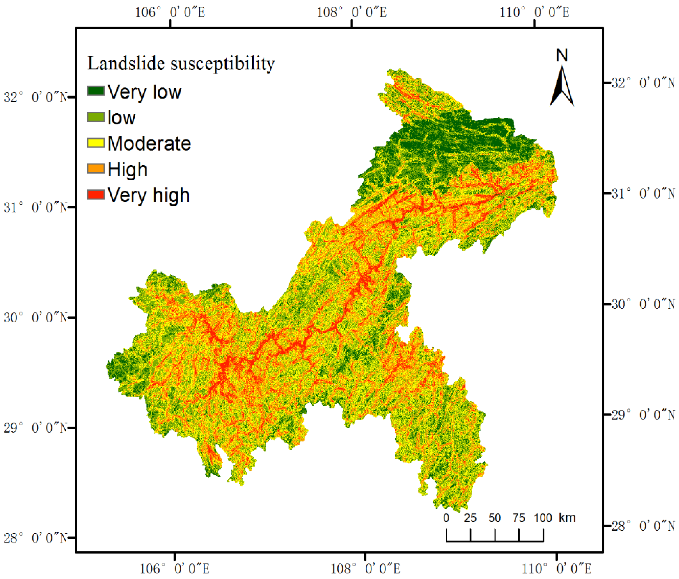
Landslide susceptibility was determined based on the total information, which was the sum of the information values of all landslide predisposing factors. Based on Jenks natural breaks optimization, the total information was divided into five classes, including very low, low, moderate, high, and very high susceptibility. Then, the landslide susceptibility map of the Chongqing study area was generated (
Figure 4).
Figure 4 shows that low susceptibility areas were mainly distributed in the southwest and northeast of the study area. High susceptibility areas were distributed in a banded pattern, along the same directions as most roads, hydrographic networks and faults. Low susceptibility areas occupied 32.96% of the study area, which was the largest proportion among all classes, while very low, moderate, high, and very high susceptibility areas accounted for 14.36%, 30.37%, 16.45,% and 5.86% of the study area, respectively.
5.2. Application of IVM-AHP
Table 4 shows the pairwise comparison matrix and weights of landslide predisposing factors determined by the analytic hierarchy process. As indicated in
Table 4, slope gradient had the maximum weight, i.e., the largest influence on landslide occurrence. The weight of aspect was the minimum, meaning that aspect had the least influence on occurrence of landslides. The weight of elevation, distance from the faults, distance from the hydrographic network, distance from the road network, rainfall, and NDVI were 0.082, 0.155, 0.059, 0.041, 0.258, and 0.035, respectively.
The consistency of the pairwise comparison matrix was tested using a consistency ratio
. The consistency index
and
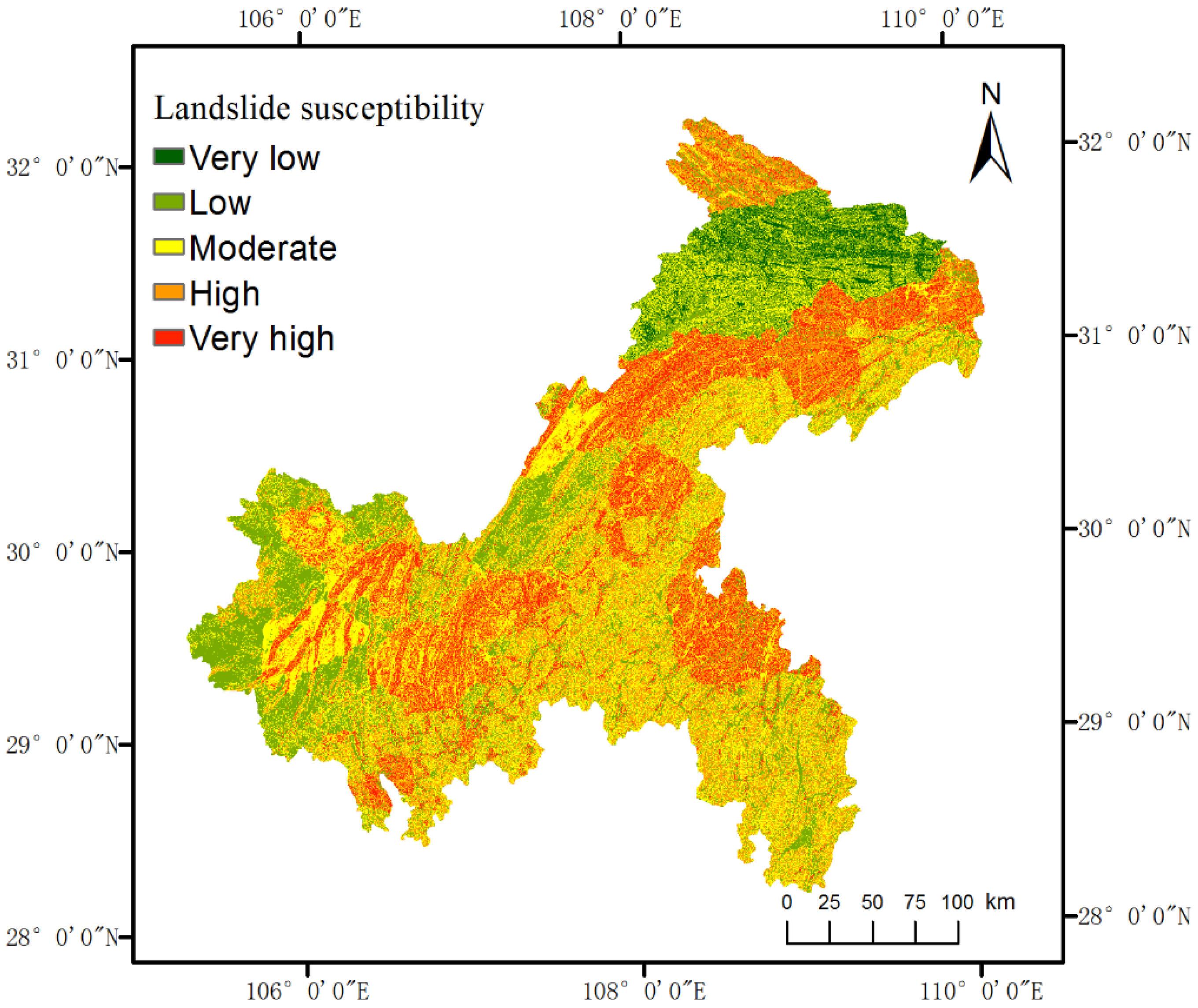
values were 0.116 and 0.082, respectively, which indicated that the pairwise comparison matrix satisfied the consistency requirement. Using the information values of each class of landslide predisposing factor derived from the IVM, the weighted information values were obtained using Equation (5) and then the landslide susceptibility map was generated (
Figure 5). As shown in
Figure 5, low susceptibility areas were mainly distributed in the southwest and northeast of the study area. High susceptibility areas were distributed in a belt pattern, which was similar to the results of the information value model shown in
Figure 4. Low susceptibility areas occupied the highest proportion, reaching 34.93%, while very low susceptibility areas took up only 3.31%. Moderate, high and very high susceptibility areas accounted for 28.70%, 21.56% and 11.49% of the study area, respectively.
5.3. Application of IVM-GC
Based on the information values of the landslide predisposing factors derived from the IVM, the landslide susceptibilities were divided into the following five classes for each predisposing factor: very low, low, moderate, high, and very high. A larger information value indicates a higher possibility of landslide occurrence, i.e., the class of higher landslide susceptibility.
Table 5 shows the landslide susceptibility classification of predisposing factors. It clearly indicates that 100–200 m elevation, 10–20° slope gradient, <600 m distance from the faults, <200 m distance from the road network, 1100–1200 mm/year rainfall, <1000 m distance from the hydrographic network, the northwest exposure aspect, and <0.55 NDVI had the highest landslide susceptibility, i.e., the very high class. In contrast, <100 m elevation, <5° slope gradient, >2400 m distance from the faults, >800 m distance from the road network, <1000 mm/year rainfall, >4000 m distance from the hydrographic network, flat aspect, and >0.85 NDVI fell into the very low susceptibility class.
After normalizing the data, the clustering weights of landslide predisposing factors were calculated using Equation (10). The results shown in
Table 6 indicate that the clustering weight (0.222) of the elevation was the maximum, while the distance from the faults had the lowest clustering weight (0.048). The weights of slope gradient, distance from road network, rainfall, distance from hydrographic network, aspect, and NDVI were 0.074, 0.177, 0.083, 0.117, 0.092, and 0.187, respectively.
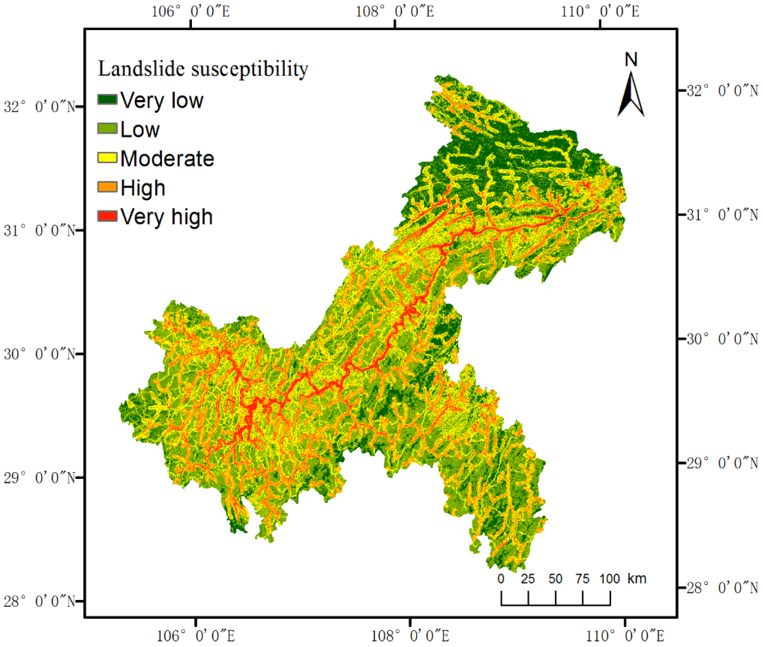
Subsequently, for each study unit, by calculating the clustering coefficient, the clustering vector was generated. The susceptibility class that each study unit belonged to was finally determined with Equation (13) and the resulting landslide susceptibility map of Chongqing is shown in
Figure 6.
As shown in
Figure 6, low susceptibility areas occupied 39.78% of the study area, followed by 23.44% for moderate susceptibility areas. Very low, high, and very high susceptibility areas accounted for 14.77%, 17.81% and 4.20% of the study area, respectively. In addition, low susceptibility areas were mainly distributed in the southwest and northeast of the area. High susceptibility areas were distributed in a banded pattern, similar to the result of information value model shown in
Figure 4.
5.4. Model Validation
In this study, the generated susceptibility maps were evaluated using a receiver operating characteristics (ROC) curve. In addition, Wilcoxon signed-rank test was used to check if the spatial pattern of the landslide susceptibility zones generated by the three models were similar.
5.4.1. Receiver Operating Characteristics Curve
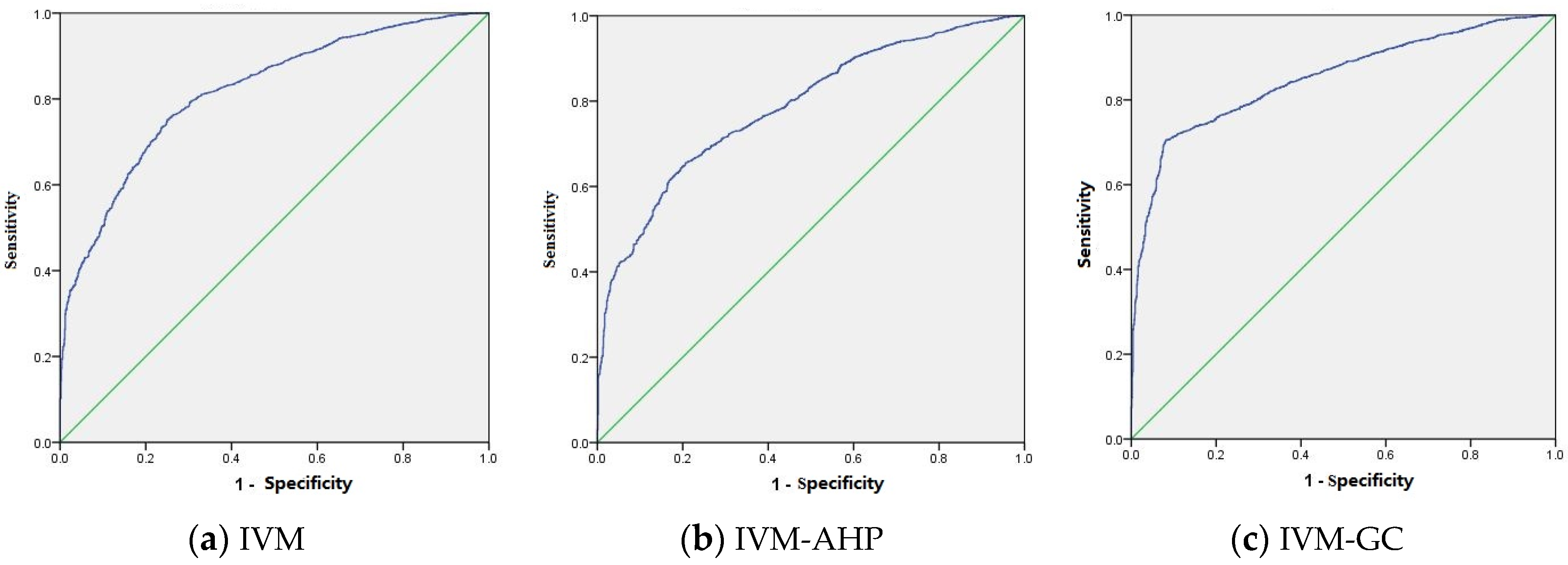
In this study, using the ROC curve, the success rate and prediction rate were calculated to assess the model accuracy and prediction ability of the three models. The success rate was obtained by comparing the 5905 landslides used for model training with the generated landslide susceptibility map (
Figure 7). As shown in
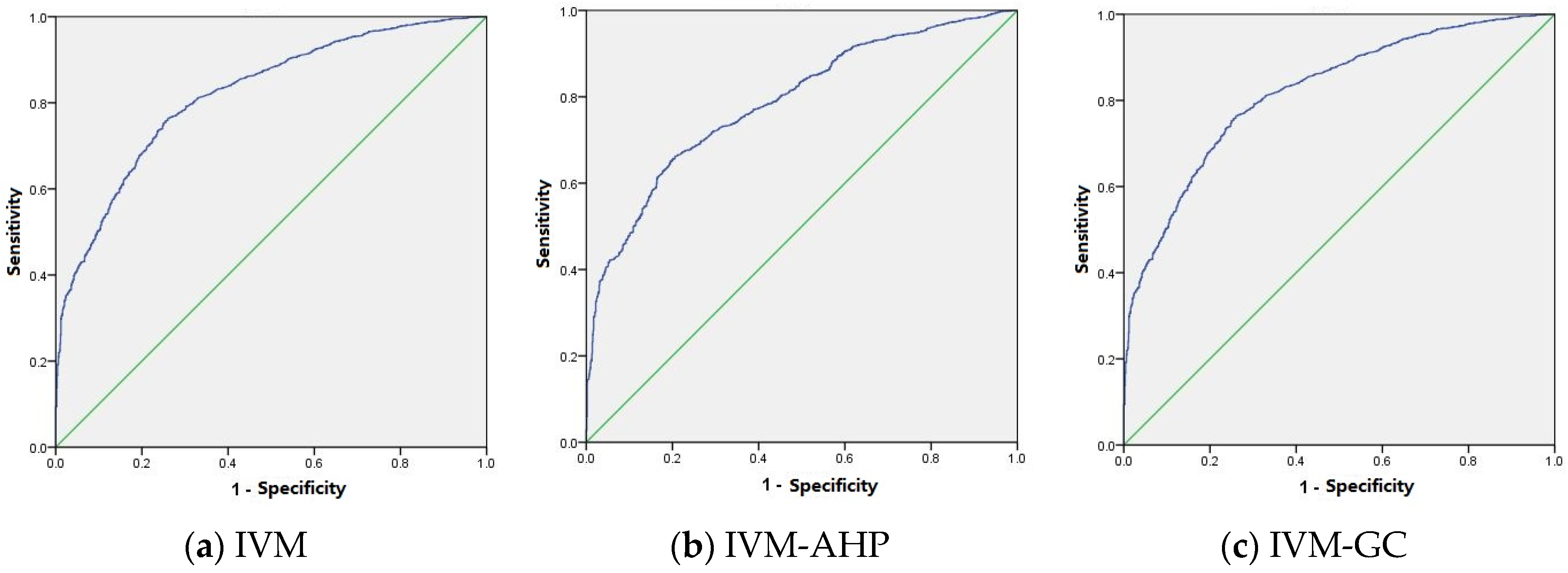
Figure 7, the x-axis represented the proportion of areas classified as landslide prone zones that are actually not. The y-axis represented the proportion of landslide zones classified as landslide prone areas. The AUC values of the IVM, IVM-AHP, and IVM-GC were 0.818, 0.787, and 0.852, respectively. Therefore, the model accuracies of the IVM, IVM-AHP, and IVM-GC were 81.8%, 78.7% and 85.2%, respectively. IVM-GC had a better performance in model construction than the IVM and IVM-AHP. The remaining 2530 (30%) landslides were compared with the landslide susceptibility map to calculate the prediction rate (
Figure 8). The AUC value of the IVM was 0.820, the AUC value of the IVM-AHP was 0.787, and the AUC value of the IVM-GC was 0.854. Therefore, the prediction accuracies of the IVM, IVM-AHP and IVM-GC were 82.0%, 78.7% and 85.4%, respectively. IVM-GC had the largest AUC value, while IVM-AHP had the smallest AUC value. Thus, IVM-GC had a better prediction capability than the IVM and IVM-AHP.
By comparing the results shown in
Figure 7 and
Figure 8, the AUC value of IVM-GC was the largest, followed by IVM, and IVM-AHP had the lowest value in both
Figure 7 and
Figure 8. It was shown that the success rate curve was similar to the prediction rate curve. In addition, the AUC values of the three models were all larger than 0.7, which suggested that the three models performed well for evaluating the landslide susceptibility of Chongqing. Among them, the AUC of IVM-GC is the largest, which indicated that IVM-GC was a relatively good method for landslide susceptibility mapping in the study area in comparison to the other two models.
5.4.2. Wilcoxon Signed-Rank Test
Using SPSS Statistics 22 software, the p-value was calculated to determine statistically significant differences (p-value < 0.05). By comparing the landslide susceptibility classification of IVM with the landslide susceptibility classification of IVM-GC in the same location, the p-value was 0.131. A comparison between the landslide susceptibility classification of IVM and IVM-AHP had a p-value of 0.458. For the comparison between the landslide susceptibility classification of IVM-GC and IVM-AHP, the p-value was 0.544. All p-values of the three comparison results were larger than 0.05. Therefore, we conclude that the landslide susceptibility mapping results of the three models had no statistically significant differences.
6. Discussion
For each landslide predisposing factor, information values vary among different classes (
Table 3). The class with the largest information value has the highest possibility of landslide development. Each of the predisposing factors makes its own contribution to landslide occurrence, and, hence, landslides are caused by a combination of predisposing factors. According to the results of the information values shown in
Table 3, the combination of landslide predisposing factors, including 100–200 m elevation, 10°–20° slope gradient, <600 m distance from the faults, <200 m distance from the road network, 1100–1200 mm/year rainfall, <1000 m distance from the hydrographic network, the northwest exposure aspect, and <0.55 NDVI, had the largest total information value and made the greatest contribution to landslide occurrence. With respect to the correlation of the variables, we have checked whether the factors used are independent from each other by utilizing a multicollinerarity test. The results show that there is a certain multicollinearity among these factors. However, some studies indicated that multicollinearity does not affect the goodness of fit and the goodness of prediction [
61].
In this paper, landslide susceptibility was reclassified into the following five classes: very low, low, moderate, high, and very high. Landslide susceptibility maps were produced using the following three different methods: IVM, IVM-AHP, and IVM-GC. In these maps, high susceptibility areas were basically distributed along the northeast to southwest direction in the study area. The high susceptibility areas were close to the geological structure, road network and hydrographic network and were mostly located in moderate slope gradient areas, where the information values were higher.
AUC was selected to evaluate the success rate and prediction rate of the three landslide susceptibility models. Theoretically, the model with the largest AUC value is the best. Based on the validation results, all three models performed well for evaluating landslide susceptibility, since their AUC values were all larger than 0.7. In addition, both success rate and prediction rate of IVM-GC are the largest, compared to IVM and IVM-AHP. Therefore, IVM-GC had a better performance than the other two models in the study area. IVM regards all landslide predisposing factors the same level of importance and assigns an equal weight to each factor. The criteria to construct the comparison pairwise of predisposing factors depend on the experience of researcher, which is subjective and is the main disadvantage of IVM-AHP. Moreover, IVM-GC inherits the advantages of the information value model, which can obtain the relative weights of different classes for each landslide predisposing factor, and appropriately determine the weights of the predisposing factors. However, the classification of each predisposing factor was based on literature and may not be the best for this case. Therefore, in future research, the effects of predisposing factor classification on landslide susceptibility assessment should be studied and an objective classification method should be advanced. There are many earthquake-induced landslides in Northwestern Chongqing; however, due to the limitation of the data, we did not use earthquakes as a predisposing factor in our model. Thus, earthquakes should be considered in future research [
62]. In addition, landslide susceptibility should be performed considering the different landslide typologies and a separation between landslide triggering conditions. Moreover, the study unit of this paper was 30 × 30 m, which was not sufficiently linked to the topography and geomorphology. In contrast, the slope unit is more related to the geomorphology, which is defined as a unit between the ridge and valley. Hence, future studies should use the slope unit as the study unit. Furthermore, landslide areas were not used to validate the landslide susceptibility models, which could be a source of uncertainty. Further studies should take this into account.
The Wilcoxon signed-rank tests indicated that the landslide susceptibility mapping results of the three models had no statistically significant differences in the spatial pattern of landslide susceptibility zones. This suggests that the prediction results of the three models were similar because these models were all based on the information value.
7. Conclusions
This paper proposes an improved information value model based on gray clustering for landslide susceptibility assessment. Using slope gradient, aspect, rainfall, elevation, distance from the road network, distance from the hydrographic network, distance from the faults, and NDVI as landslide predisposing factors, landslide susceptibility maps of Chongqing, China were generated based on three models, i.e., IVM, IVM-AHP, and IVM-GC.
The resultant landslide susceptibility maps show that the high susceptibility areas are mainly distributed along the northeast to southwest direction in the study area. The Wilcoxon signed-rank tests indicated that the spatial pattern of the landslide susceptibility zones generated by the three models had no statistically significant differences. ROC was used to evaluate these models by comparing the success rate and prediction rate. By calculating the AUC values of the success rate and the prediction rate curves, all three models performed well in evaluating the landslide susceptibility of Chongqing. Among them, IVM-GC had the best performance for landslide susceptibility mapping in the study area. IVM-GC not only inherits the advantages of the information value model, which can obtain the relative weights of different classes of each landslide predisposing factor but can also appropriately determine the weights of predisposing factors.
In our newly improved IVM-GC model, however, the classification of each predisposing factor was based on relevant literature and may not be the best for this case. Therefore, further studies should explore the effects of predisposing factor classification on landslide susceptibility assessment, and an objective classification method should be advanced. In addition, earthquakes should be used as a predisposing factor in our model and the different landslide typologies and a separation between landslide triggering conditions should be considered. Furthermore, the slope unit, which is more related to the topography and geomorphology, should be used as the study unit for future research.
Acknowledgments
The research is supported by National Nature Science Foundation of China (project No. 41671380), the key project of National Nature Science Foundation of China (project No. 41531180) and is funded by the Foundation of Key Laboratory for Geo-Environmental Monitoring of Coastal Zone of the National Administration of Surveying, Mapping and Geoinformation. We also want to express our sincere thanks to the editor and the anonymous reviewers for their valuable comments and suggestions for this paper.
Author Contributions
Qianqian Ba, Yumin Chen, and Susu Deng conceived and designed the experiments; Qianjiao Wu, Jiaxin Yang and Jingyi Zhang analyzed the data; Yumin Chen and Susu Deng contributed reagents/materials/analysis tools; Qianqian Ba, Yumin Chen, Susu Deng and Qianjiao Wu performed the experiments; Qianqian Ba, Yumin Chen, Susu Deng and Qianjiao Wu wrote the paper; Jiaxin Yang and Jingyi Zhang drew graphs for the paper.
Conflicts of Interest
The authors declare no conflict of interest.
References
- Devkota, K.C.; Regmi, A.D.; Pourghasemi, H.R. Landslide susceptibility mapping using certainty factor, index of entropy and logistic regression models in GIS and their comparison at Mugling–Narayanghat road section in Nepal Himalaya. Nat. Hazards 2013, 65, 135–165. [Google Scholar] [CrossRef] [Green Version]
- Zhou, S.H.; Chen, G.Q.; Fang, L.G. Distribution pattern of landslides triggered by the 2014 Ludian Earthquake of China: Implications for regional threshold topography and the seismogenic fault identification. ISPRS Int. J. Geo-Inf. 2016. [Google Scholar] [CrossRef]
- Barredo, J.; Benavides, A.; Hervás, J. Comparing heuristic landslide hazard assessment techniques using GIS in the Tirajana basin, Gran Canaria Island, Spain. Int. J. Appl. Earth Obs. 2000, 2, 9–23. [Google Scholar] [CrossRef]
- Maharaj, R.J. Landslide processes and landslide susceptibility analysis from an upland watershed: A case study from St. Andrew, Jamaica, West Indies. Eng. Geol. 1993, 34, 53–79. [Google Scholar] [CrossRef]
- Clerici, A.; Perego, S.; Tellini, C. A procedure for landslide susceptibility zonation by the conditional analysis method. Geomorphology 2002, 48, 349–364. [Google Scholar] [CrossRef]
- Akcay, O. Landslide fissure inference assessment by ANFIS and logistic regression using UAS-based photogrammetry. ISPRS Int. J. Geo-Inf. 2015, 4, 2131–2158. [Google Scholar] [CrossRef]
- Bui, D.T.; Pradhan, B.; Lofman, O. Landslide susceptibility assessment in the Hoa Binh province of Vietnam: A comparison of the Levenberg–Marquardt and Bayesian regularized neural networks. Geomorphology 2012, 171, 12–29. [Google Scholar]
- Zhu, A.X.; Wang, R.; Qiao, J.; Qin, C.Z.; Chen, Y.; Liu, J. An expert knowledge-based approach to landslide susceptibility mapping using GIS and fuzzy logic. Geomorphology 2014, 214, 128–138. [Google Scholar] [CrossRef]
- Christos, C.; Maria, F.; Christos, P. GIS supported landslide susceptibility modeling at regional scale: An expert-based fuzzy weighting method. ISPRS Int. J. Geo-Inf. 2014, 3, 523–539. [Google Scholar]
- Yilmaz, I. Landslide susceptibility mapping using frequency ratio, logistic regression, artificial neural networks and their comparison: A case study from Kat landslides (Tokat—Turkey). Comput. Geosci. 2009, 35, 1125–1138. [Google Scholar] [CrossRef]
- Ermini, L.; Catani, F.; Casagli, N. Artificial neural networks applied to landslide susceptibility assessment. Geomorphology 2005, 66, 327–343. [Google Scholar] [CrossRef]
- Gorsevski, P.V.; Gessler, P.E.; Foltz, R.B. Spatial prediction of landslide hazard using logistic regression and ROC analysis. Trans. GIS 2006, 10, 395–415. [Google Scholar] [CrossRef]
- Bai, S.; Lu, G.; Wang, J. GIS-based rare events logistic regression for landslide-susceptibility mapping of Lianyungang, China. Environ. Earth Sci. 2010, 62, 139–149. [Google Scholar] [CrossRef]
- Terence, L.; Suzana, D.; Margaret, S. Integration of multicriteria evaluation and cellular automata methods for landslide simulation modelling. Geomat. Nat. Hazards Risk 2013, 4, 355–375. [Google Scholar]
- Kayastha, P.; Dhital, M.R.; Smedt, F.D. Application of the analytical hierarchy process (AHP) for landslide susceptibility mapping: A case study from the Tinau Watershed, West Nepal. Comput. Geosci. 2013, 52, 398–408. [Google Scholar] [CrossRef]
- Romeijn, H.; Faggian, R.; Diogo, V.; Sposito, V. Evaluation of deterministic and complex analytical hierarchy process methods for agricultural land suitability analysis in a changing climate. ISPRS Int. J. Geo-Inf. 2016. [Google Scholar] [CrossRef]
- Corominas, J.; Westen, C.V.; Frattini, P.; Cascini, L.; Malet, J.P.; Fotopoulou, S. Recommendations for the quantitative analysis of landslide risk. Bull. Eng. Geol. Environ. 2014, 73, 209–263. [Google Scholar] [CrossRef] [Green Version]
- Xu, W.; Yu, W.; Jing, S. Debris flow susceptibility assessment by GIS and information value model in a large-scale region, Sichuan Province (China). Nat. Hazards 2013, 65, 1379–1392. [Google Scholar] [CrossRef]
- Chen, W.; Li, W.; Hou, E. Landslide susceptibility mapping based on GIS and information value model for the Chencang District of Baoji, China. Arabian J. Geosci. 2014, 7, 4499–4511. [Google Scholar] [CrossRef]
- Zhu, C.; Wang, X. Landslide susceptibility mapping: A comparison of information and weights-of-evidence methods in Three Gorges Area. In Proceedings of the International Conference on Environmental Science & Information Application Technology, Wuhan, China, 4–5 July 2009.
- Chen, T.; Niu, R.; Jia, X. A comparison of information value and logistic regression models in landslide susceptibility mapping by using GIS. Environ. Earth Sci. 2016, 75, 1–16. [Google Scholar] [CrossRef]
- Jiang, L.; Liu, D.; Jiang, Y. Landside susceptibility assessment based on weighted information value model: A case study of Wenchuan earthquake 10 degree region. In Proceedings of the International Conference on Agro-Geoinformatics, Beijing, China, 11–14 August 2014; pp. 1–4.
- Sharma, L.P.; Patel, N.; Ghose, M.K. Development and application of Shannon’s entropy integrated information value model for landslide susceptibility assessment and zonation in Sikkim Himalayas in India. Nat. Hazards 2015, 75, 1555–1576. [Google Scholar] [CrossRef]
- Xiao, L. Relative analysis between strong rainfall process and geological hazards Chongqing City. Chin. J. Geol. Hazard Control 1995, 6, 39–42. [Google Scholar]
- Tamrakar, N.K.; Yokota, S.; Osaka, O. A toppled structure with sliding in the Siwalik Hills, Midwestern Nepal. Eng. Geol. 2002, 64, 339–350. [Google Scholar] [CrossRef]
- Masson, D.G.; Harbitz, C.B.; Wynn, R.B.; Pedersen, G.; Lovholt, F. Submarine landslides: Processes, triggers and hazard prediction. Philos. Trans. R. Soc. Lond. Ser. A Math. Phys. Eng. Sci. 2006, 364, 2009–2039. [Google Scholar] [CrossRef] [PubMed]
- Reis, S.; Yalcin, A.; Atasoy, M.; Nisanci, R.; Bayrak, T.; Erduran, M. Remote sensing and GIS-based landslide susceptibility mapping using frequency ratio and analytical hierarchy methods in Rize Province (NE Turkey). Environ. Earth Sci. 2012, 66, 2063–2073. [Google Scholar] [CrossRef]
- Pourghasemi, H.R.; Pradhan, B.; Gokceoglu, C. Application of fuzzy logic and analytical hierarchy process (AHP) to landslide susceptibility mapping at Haraz Watershed, Iran. Nat. Hazards 2012, 63, 1–32. [Google Scholar] [CrossRef]
- Foumelis, M.; Lekkas, E.; Parcharidis, I. Landslide susceptibility mapping by GIS-based qualitative weighting procedure in Corinth area. Bull. Geol. Soc. Greece 2004, 36, 904–912. [Google Scholar]
- Saad, B.; Mitri, H.; Poorooshasb, H. 3D FE analysis of flexible pavement with Geosynthetic reinforcement. J. Transp. Eng. 2006, 132, 402–415. [Google Scholar] [CrossRef]
- Ma, F.; Wang, J.; Yuan, R.; Zhao, H.; Guo, J. Application of analytical hierarchy process and least-squares method for landslide susceptibility assessment along the Zhong-Wu natural gas pipeline, China. Landslides 2013, 10, 481–492. [Google Scholar] [CrossRef]
- Yalcin, A. GIS-based landslide susceptibility mapping using analytical hierarchy process and bivariate statistics in Ardesen (Turkey): Comparisons of results and confirmations. Catena 2008, 72, 1–12. [Google Scholar] [CrossRef]
- Glade, T. Landslide occurrence as a response to land use change: A review of evidence from New Zealand. Catena 2003, 51, 297–314. [Google Scholar] [CrossRef]
- Chen, Y.R.; Ni, P.N.; Chen, J.W.; Hsieh, S.C. The application of remote sensing technology to the interpretation of land use for rainfall-induced landslides based on genetic algorithms and artificial neural networks. IEEE J. Sel. Top. Appl. Earth Obs. Remote Sens. 2009, 2, 87–95. [Google Scholar] [CrossRef]
- Anbalagan, R. Landslide hazard evaluation and zonation mapping in mountainous terrain. Eng. Geol. 1992, 32, 269–277. [Google Scholar] [CrossRef]
- Yin, K.L.; Yan, T.Z. Statistical Prediction models for slope instability of metamorphosed rocks. In Proceedings of the 5th International Symposium on Landslides, Lausanne, Switzerland, 10–15 July 1988.
- Wang, Q.; Wang, D.; Huang, Y.; Wang, Z.; Zhang, L.; Guo, Q. Landslide susceptibility mapping based on selected optimal combination of landslide predisposing factors in a large catchment. Sustainability 2015, 7, 16653–16669. [Google Scholar] [CrossRef]
- Yan, T.Z. Recent advances of quantitative prognoses of landslide in China. In Proceedings of the 5th International Symposium on Landslides, Lausanne, Switzerland, 10–15 July 1988.
- Chen, J.; Yang, S.T.; Li, H.W.; Zhang, B.; Lv, J.R. Research on geographical environment unit division based on the method of natural breaks (Jenks). Int. Arch. Photogramm. Remote Sens. Spat. Inf. Sci. 2013, XL-4/W3, 47–50. [Google Scholar] [CrossRef]
- Hummel, J.M.; Omta, S.W.F.; Rossum, W.V.; Verkerke, G.J.; Rakhorst, G. The analytic hierarchy process: An effective tool for a strategic decision of a multidisciplinary research center. Knowl. Technol. Policy 2001, 11, 41–63. [Google Scholar] [CrossRef]
- Zhang, H. The analysis of the reasonable structure of water conservancy investment of capital construction in china by AHP method. Water Resour. Manag. 2008, 23, 1–18. [Google Scholar] [CrossRef]
- Ayalew, L.; Yamagishi, H.; Ugawa, N. Landslide susceptibility mapping using GIS-based weighted linear combination, the case in Tsugawa area of Agano River, Niigata Prefecture, Japan. Landslides 2004, 1, 73–81. [Google Scholar] [CrossRef]
- Bathrellos, G.D.; Skilodimou, H.D.; Chousianitis, K.; Youssef, A.M.; Pradhan, B. Suitability estimation for urban development using multi-hazard assessment map. Sci. Total Environ. 2017, 575, 119–134. [Google Scholar] [CrossRef] [PubMed]
- Saaty, T.L.; Vargas, L.G. Models, Methods, Concepts & Applications of the Analytic Hierarchy Process, 1st ed.; Springer: New York, NY, USA, 2001; pp. 159–172. [Google Scholar]
- Chhetri, S.; Kayastha, P. Manifestation of an analytic hierarchy process (AHP) model on fire potential zonation mapping in Kathmandu Metropolitan City, Nepal. ISPRS Int. J. Geo-Inf. 2015, 4, 400–417. [Google Scholar] [CrossRef]
- Bathrellos, G.D.; Karymbalis, E.; Skilodimou, H.D.; Gaki-Papanastassiou, K.; Baltas, E.A. Urban flood hazard assessment in the basin of Athens Metropolitan city, Greece. Environ. Earth Sci. 2016. [Google Scholar] [CrossRef]
- Saaty, T.L. The Analytic Hierarchy Process, Planning, Piority Setting, Resource Allocation; McGraw-Hill: New York, NY, USA, 1980. [Google Scholar]
- Bunruamkaew, K.; Murayam, Y. Site suitability evaluation for ecotourism using GIS & AHP: A case study of Surat Thani Province, Thailand. Procedia 2011, 21, 269–278. [Google Scholar]
- Rozos, D.; Bathrellos, G.D.; Skilodimou, H.D. Comparison of the implementation of rock engineering system (RES) and analytic hierarchy process (AHP) methods, based on landslide susceptibility maps, compiled in GIS environment: A case study from the eastern Achaia County of Peloponnesus, Greece. Environ. Earth Sci. 2011, 63, 49–63. [Google Scholar] [CrossRef]
- Bathrellos, G.D.; Gaki-Papanastassiou, K.; Skilodimou, H.D.; Papanastassiou, D.; Chousianitis, K.G. Potential suitability for urban planning and industry development using natural hazard maps and geological–geomorphological parameters. Environ. Earth Sci. 2012, 66, 537–548. [Google Scholar] [CrossRef]
- Wei, G.; Feng, X.T. Study on displacement predication of landslide based on grey system and evolutionary neural network. Rock Soil Mech. 2004, 25, 275. [Google Scholar]
- Xie, N.; Xin, J.; Liu, S. China’s regional meteorological disaster loss analysis and evaluation based on grey cluster model. Nat. Hazards 2014, 71, 1067–1089. [Google Scholar] [CrossRef]
- Li, C.; Wu, S.; Zhu, Z. The assessment of submarine slope instability in Baiyun Sag using gray clustering method. Nat. Hazards 2014, 74, 1179–1190. [Google Scholar] [CrossRef]
- García-Rodríguez, M.J.; Malpica, J.A.; Benito, B.; Díaz, M. Susceptibility assessment of earthquake-triggered landslides in El Salvador using logistic regression. Geomorphology 2008, 95, 172–191. [Google Scholar] [CrossRef] [Green Version]
- Tsangaratos, P.; Ilia, I.; Hong, H.; Chen, W.; Xu, C. Applying information theory and GIS-based quantitative methods to produce landslide susceptibility maps in Nancheng County, China. Landslides 2016. [Google Scholar] [CrossRef]
- Myronidis, D.; Papageorgiou, C.; Theophanous, S. Landslide susceptibility mapping based on landslide history and analytic hierarchy process (AHP). Nat. Hazards 2016, 81, 254–263. [Google Scholar] [CrossRef]
- Cimenti, C.; Erwa, W.; MuLler, W.; Resch, B. The role of immature granulocyte count and immature myeloid information in the diagnosis of neonatal sepsis. Intech 2012, 50, 1429–1432. [Google Scholar]
- Concepts & Applications of Inferential Statistics. Available online: http://vassarstats.net/textbook (accessed on 10 January 2017).
- Chen, Y.; Ba, Q.; Wu, Q.; Li, X. Landslide susceptibility evaluation based on GIS and information value model. In Proceedings of the 2015 4th National Conference on Electrical, Electronics and Computer Engineering (NCEECE 2015), Xi’an, China, 12–13 December 2015.
- Salvatore, R.; Alessio, V. Neural network aided evaluation of landslide susceptibility in southern Italy. Int. J. Mod. Phys. C 2012, 23, 98–108. [Google Scholar]
- Multicollinearity in Regression. Available online: http://support.minitab.com/en-us/minitab/17/topic-library/modeling-statistics/regression-and-correlation/model-assumptions/multicollinearity-in-regression/ (accessed on 10 November 2016).
- Chousianitis, K.; Del Gaudio, V.; Sabatakakis, N.; Kavoura, K.; Drakatos, G.; Bathrellos, G.D.; Skilodimou, H.D. Assessment of earthquake-induced landslide hazard in Greece: From arias intensity to spatial distribution of slope resistance demand. Bull. Seismol. Soc. Am. 2016, 106, 664–675. [Google Scholar] [CrossRef]
© 2017 by the authors; licensee MDPI, Basel, Switzerland. This article is an open access article distributed under the terms and conditions of the Creative Commons Attribution (CC-BY) license (http://creativecommons.org/licenses/by/4.0/).


