
Morphological Principal Component Analysis for Hyperspectral Image Analysis †

Abstract
:1. Introduction
2. Basics on Morphological Image Representation
2.1. Notation
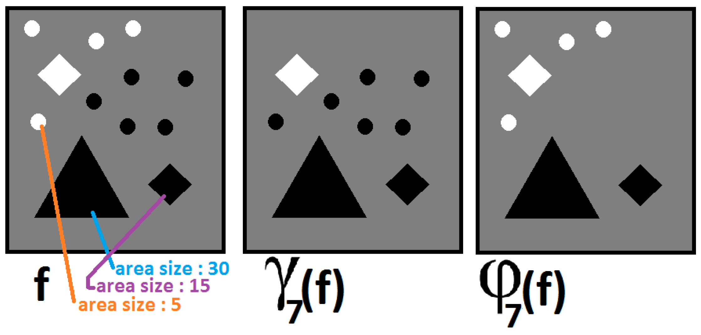
2.2. Nonlinear Scale-Spaces and Morphological Decomposition
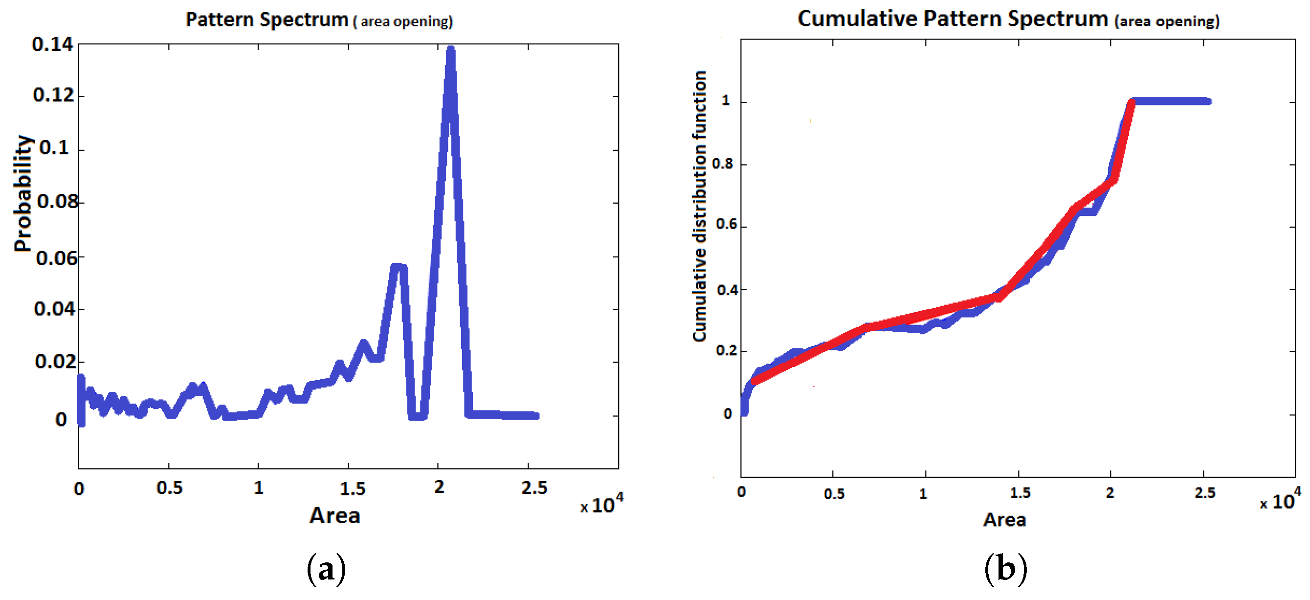
2.3. Pattern Spectrum
2.4. Grey-Scale Distance Function
3. Morphological Principal Component Analysis
3.1. Remind on Classical PCA
3.2. Covariance Matrix and Pearson Correlation Matrix
3.3. MorphPCA and Its Variants
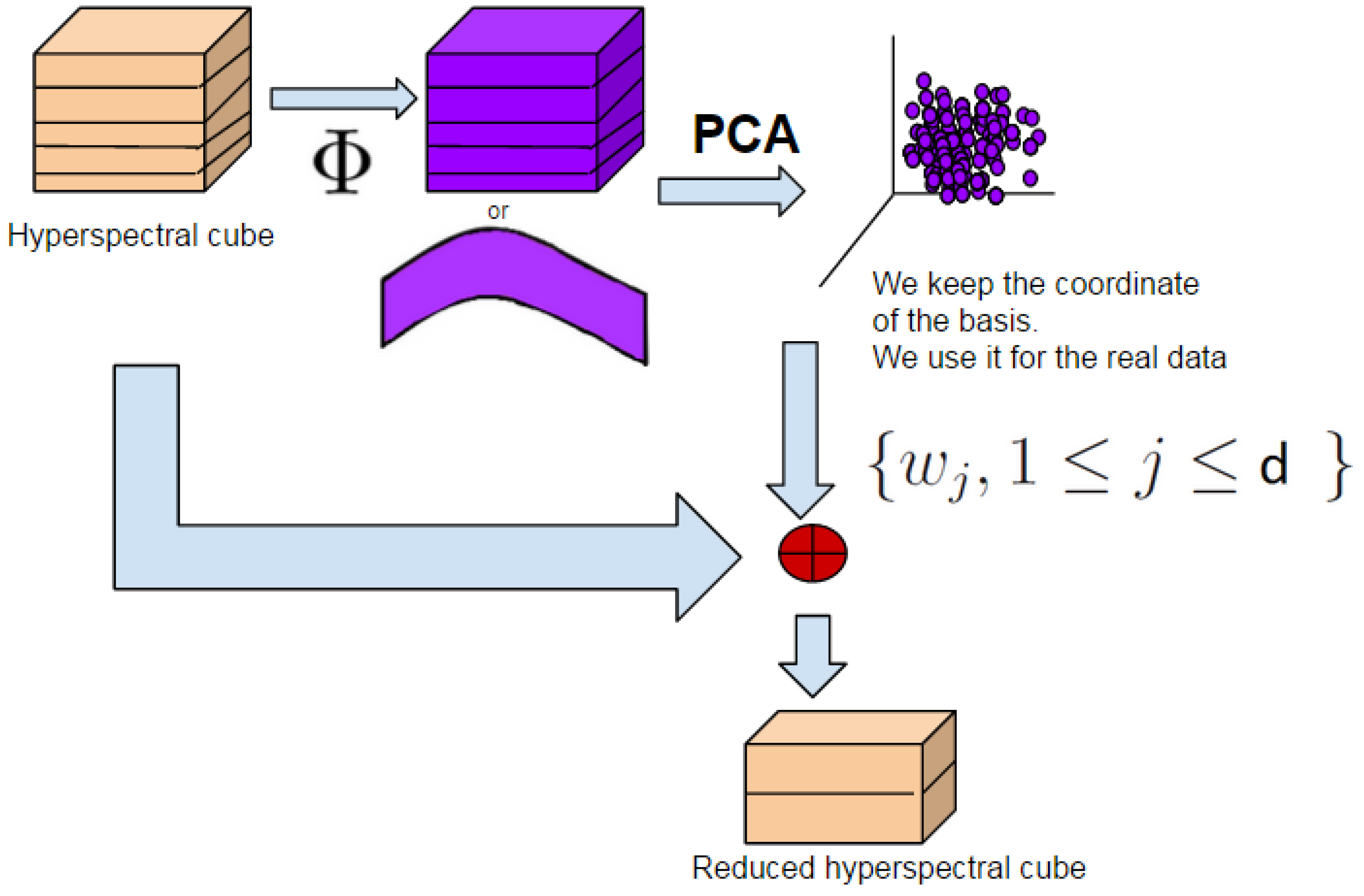
3.3.1. Scale-Space Decomposition MorphPCA
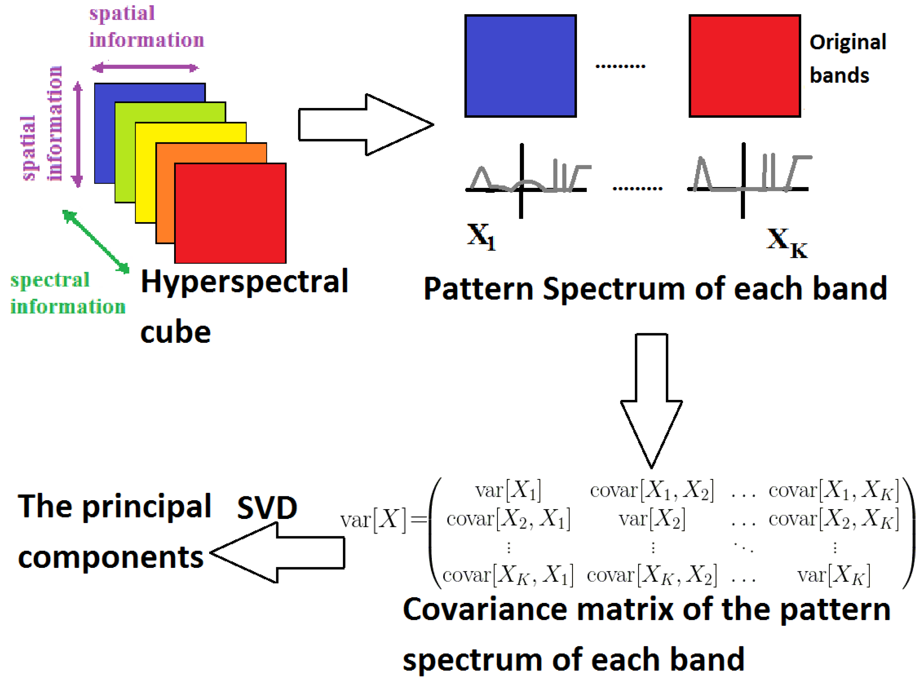
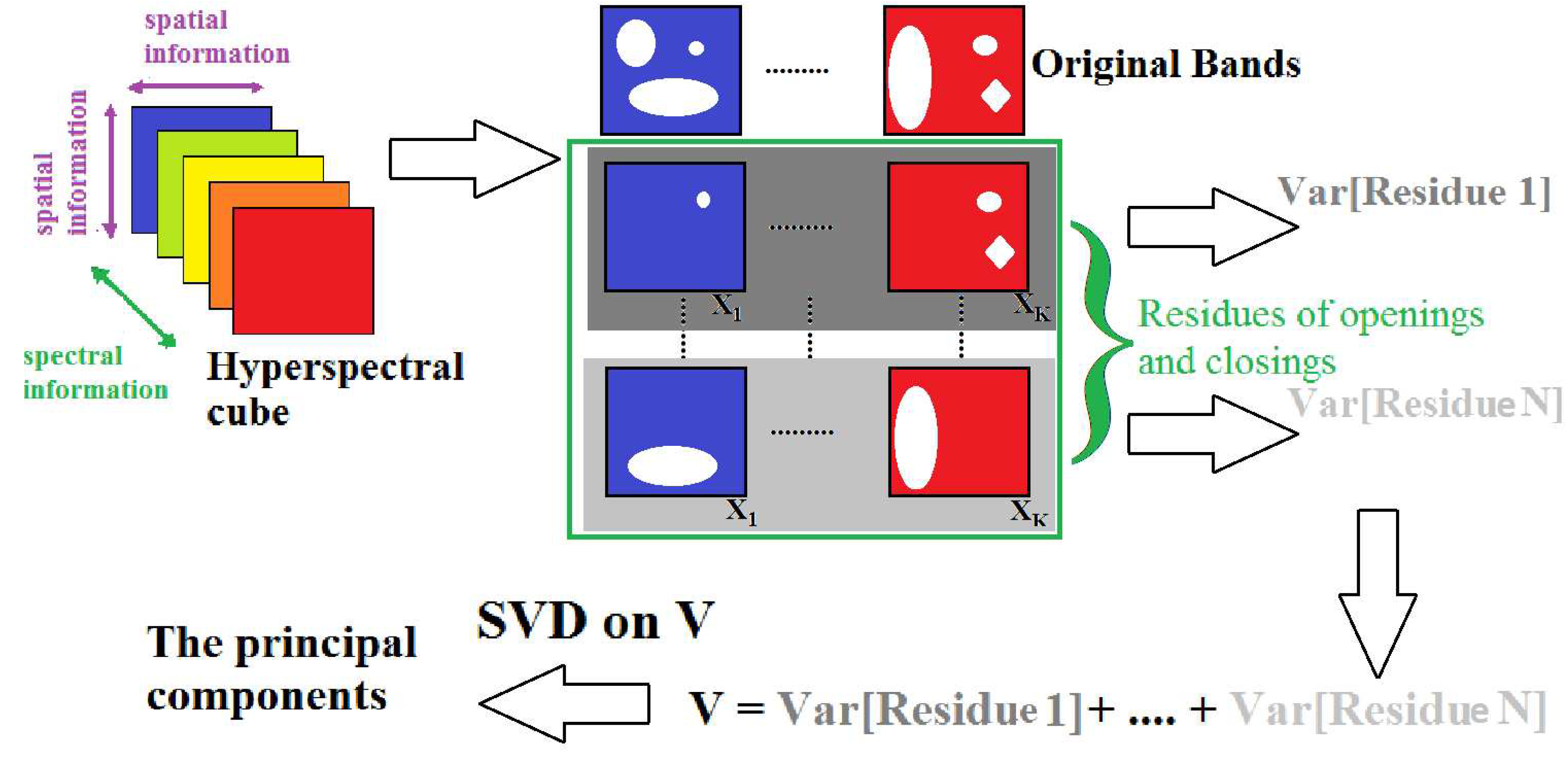
3.3.2. Pattern Spectrum MorphPCA
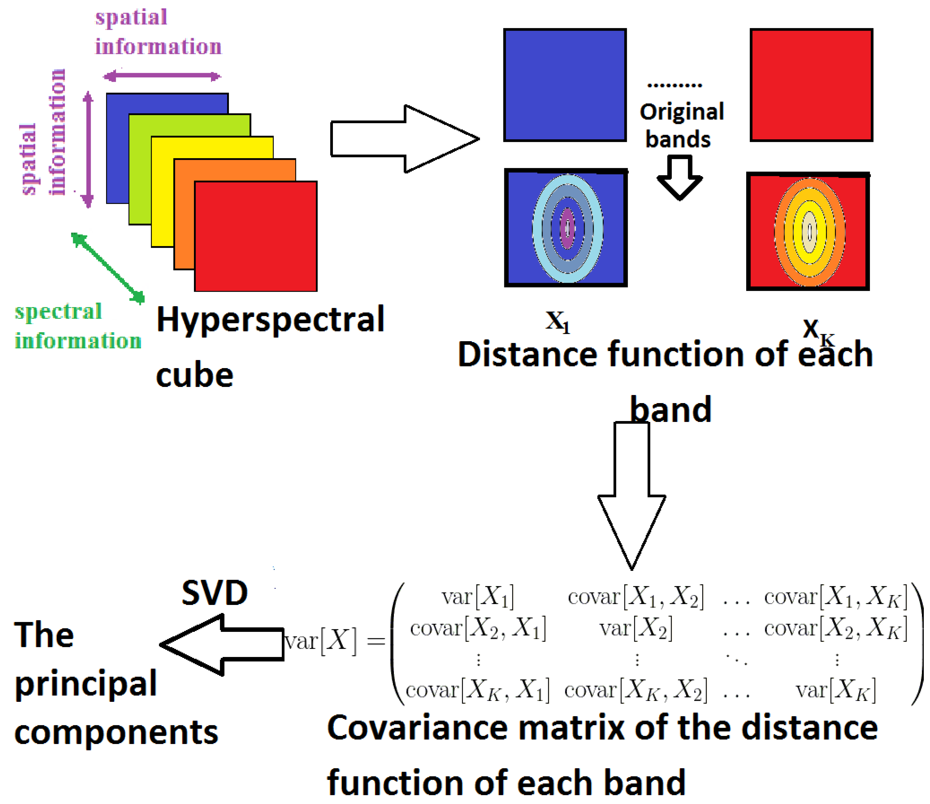
3.3.3. Distance Function MorphPCA
3.3.4. Spatial/Spectral MorphPCA
4. MorphPCA Applied to Hyperspectral Images
4.1. Criteria to Evaluate PCA vs. MorphPCA
- Local criteria.
- Criterion 1 (C1)
- The reconstructed hyperspectral image using the first d principal components should be a regularized version of in order to be more spatially sparse.
- Criterion 2 (C2)
- The reconstructed hyperspectral image using the first d principal components should preserve local homogeneity and be coherent with the original hyperspectral image .
- Criterion 3 (C3)
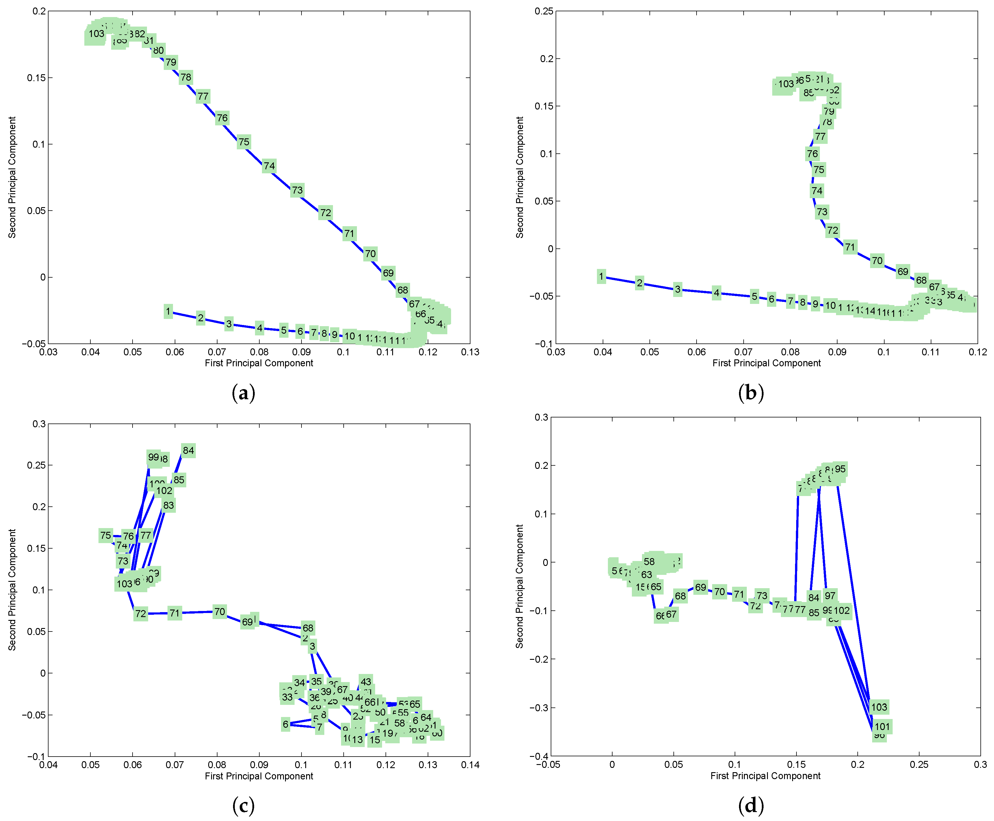
- The manifold of variables (i.e., intrinsic geometry) from the reconstructed hyperspectral image should be as similar as possible to the manifold from original hyperspectral image .
- Global criteria.
- Criterion 4 (C4)
- The number of bands d of the reduced hyperspectral image should be reduced as much as possible. It means that a spectrally sparse image is obtained.
- Criterion 5 (C5)
- The reconstructed hyperspectral image using the first d principal components should preserve the global similarity with the original hyperspectral image . Or in other words, it should be a good noise-free approximation.
- Criterion 6 (C6)
- Separability of spectral classes should be improved in the dimensionality reduced space. That involves in particular a better pixel classification.
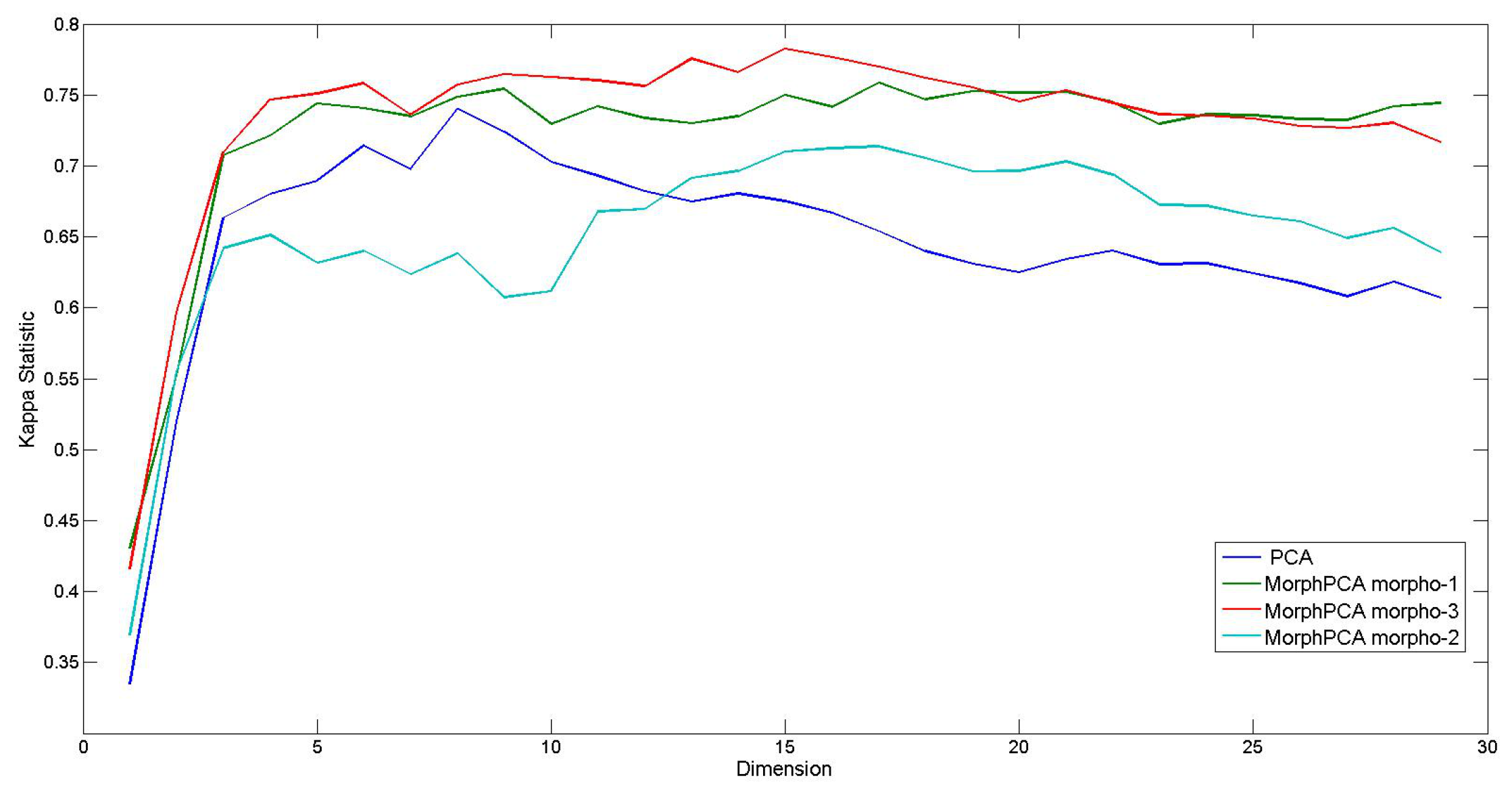
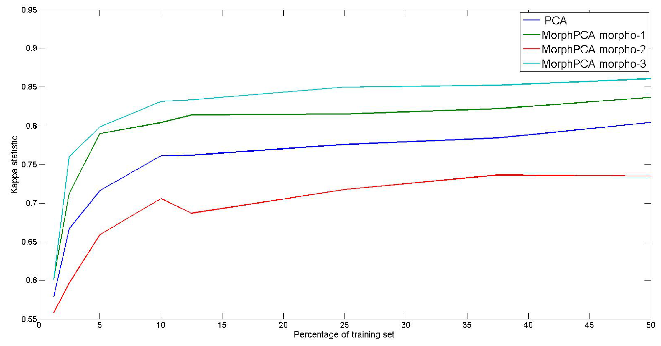
4.2. Evaluation of Algorithms
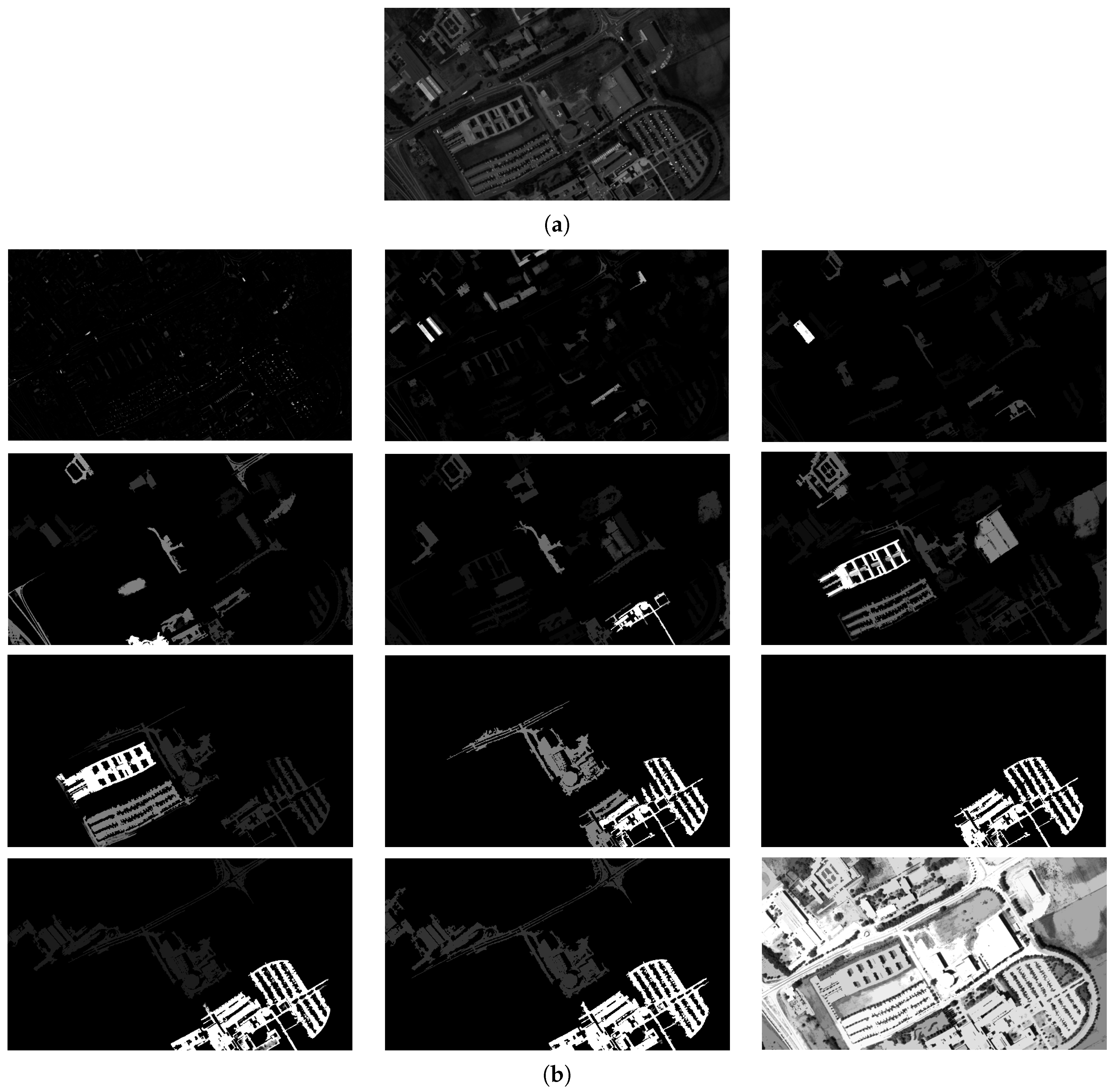
4.3. Evaluation on Hyperspectral Images
5. Conclusions
Acknowledgments
Author Contributions
Conflicts of Interest
References
- Guilfoyle, K.; Althouse, M.L.; Chang, C.I. Further investigations into the use of linear and nonlinear mixing models for hyperspectral image analysis. Proc. SPIE 2002. [Google Scholar] [CrossRef]
- Bachmann, C.; Ainsworth, T.; Fusina, R. Exploiting manifold geometry in hyperspectral imagery. IEEE Trans. Geosci. Remote Sens. 2005, 43, 441–454. [Google Scholar] [CrossRef]
- Van der Maaten, L.J.; Postma, E.O.; van den Herik, H.J. Dimensionality reduction: A comparative review. J. Mach. Learn. Res. 2009, 10, 66–71. [Google Scholar]
- Dalla Mura, M.; Benediktsson, J.; Waske, B.; Bruzzone, L. Morphological attribute profiles for the analysis of very high resolution images. IEEE Trans. Geosci. Remote Sens. 2010, 48, 3747–3762. [Google Scholar] [CrossRef]
- Fauvel, M.; Benediktsson, J.; Chanussot, J.; Sveinsson, J. Spectral and spatial classification of hyperspectral data using svms and morphological profiles. IEEE Trans. Geosci. Remote Sens. 2008, 46, 3804–3814. [Google Scholar] [CrossRef]
- Pesaresi, M.; Benediktsson, J. A new approach for the morphological segmentation of high-resolution satellite imagery. IEEE Trans. Geosci. Remote Sens. 2001, 39, 309–320. [Google Scholar] [CrossRef]
- Lefevre, S.; Chapel, L.; Merciol, F. Hyperspectral image classification from multiscale description with constrained connectivity and metric learning. In Proceedings of the 6th International Workshop on Hyperspectral Image and Signal Processing: Evolution in Remote Sensing (WHISPERS 2014), Lausannne, Switzerland, 24–27 June 2014.
- Aptoula, E.; Lefevre, S. A comparative study on multivariate mathematical morphology. Pattern Recognit. 2007, 40, 2914–2929. [Google Scholar] [CrossRef]
- Li, J.; Bioucas-Dias, J.M.; Plaza, A. Hyperspectral image segmentation using a new bayesian approach with active learning. IEEE Trans. Geosci. Remote Sens. 2011, 49, 3947–3960. [Google Scholar] [CrossRef]
- Mercier, G.; Derrode, S.; Lennon, M. Hyperspectral image segmentation with markov chain model. In Proceedings of the 2003 IEEE International Geoscience and Remote Sensing Symposium, IGARSS ’03, Toulouse, France, 21–25 July 2003; pp. 3766–3768.
- Camps-Valls, G.; Bruzzone, L. Kernel-based methods for hyperspectral image classification. IEEE Trans. Geosci. Remote Sens. 2005, 43, 1351–1362. [Google Scholar] [CrossRef]
- Camps-Valls, G.; Gomez-Chova, L.; Mu noz-Marí, J.; Vila-Francés, J.; Calpe-Maravilla, J. Composite kernels for hyperspectral image classification. IEEE Geosci. Remote Sens. Lett. 2006, 3, 93–97. [Google Scholar] [CrossRef]
- Mathieu, F.; Jocelyn, C.; Jón Atli, B. Kernel principal component analysis for the classification of hyperspectral remote sensing data over urban areas. EURASIP J. Adv. Signal Process. 2009. [Google Scholar] [CrossRef]
- Volpi, M.; Tuia, D. Spatially aware supervised nonlinear dimensionality reduction for hyperspectral data. In Proceedings of the 6th International Workshop on Hyperspectral Image and Signal Processing: Evolution in Remote Sensing (WHISPERS 2014), Lausannne, Switzerland, 24–27 June 2014.
- Velasco-Forero, S.; Angulo, J. Classification of hyperspectral images by tensor modeling and additive morphological decomposition. Pattern Recognit. 2013, 46, 566–577. [Google Scholar] [CrossRef]
- Renard, N.; Bourennane, S. Dimensionality reduction based on tensor modeling for classification methods. IEEE Trans. Geosci. Remote Sens. 2009, 47, 1123–1131. [Google Scholar] [CrossRef]
- Bakshi, B.R. Multiscale pca with application to multivariate statistical process monitoring. AIChE J. 1998, 44, 1596–1610. [Google Scholar] [CrossRef]
- Franchi, G.; Angulo, J. Comparative study on morphological principal component analysis of hyperspectral images. In Proceedings of the 6th International Workshop on Hyperspectral Image and Signal Processing: Evolution in Remote Sensing (WHISPERS 2014), Lausannne, Switzerland, 24–27 June 2014.
- I.G.D.F. Contest. Available online: http://www.grss-ieee.org/community/technical-committees/data-fusion/ (accessed on 17 December 2015).
- Vincent, L. Morphological area opening and closing for greyscale images. In Proceedings of the NATO Shape in Picture Workshop, Driebergen, The Netherlands, May 1993.
- Serra, J. Image Analysis and Mathematical Morphology; Academic Press, Inc.: Orlando, FL, USA, 1983. [Google Scholar]
- Cavallaro, G.; Falco, N.; Dalla Mura, M.; Bruzzone, L.; Benediktsson, J.A. Automatic threshold selection for profiles of attribute filters based on granulometric characteristic functions. In Mathematical Morphology and Its Applications to Signal and Image Processing; Springer: Reykjavik, Islande, 2015; pp. 169–181. [Google Scholar]
- Maragos, P. Pattern spectrum and multiscale shape representation. IEEE Trans. Pattern Anal. Mach. Intell. 1989, 11, 701–716. [Google Scholar] [CrossRef]
- Matheron, G. Random Sets and Integral Geometry; John Wiley & Sons: New York, NY, USA, 1975. [Google Scholar]
- Soille, P. Morphological Image Analysis: Principles and Applications; Springer Science & Business Media: Berlin, Germany, 2013. [Google Scholar]
- Molchanov, I.S.; Teran, P. Distance transforms for real-valued functions. J. Math. Anal. Appl. 2003, 278, 472–484. [Google Scholar] [CrossRef]
- Goshtasby, A.A. Similarity and dissimilarity measures. In Image Registration; Springer: Berlin, Germany, 2012; pp. 7–66. [Google Scholar]
- Huntington, E.V. Mathematics and statistics, with an elementary account of the correlation coefficient and the correlation ratio. Am. Math. Mon. 1919, 26, 421–435. [Google Scholar] [CrossRef]
- Baddeley, A. Errors in binary images and an lp version of the hausdorff metric. Nieuw Archief voor Wiskunde 1992, 10, 157–183. [Google Scholar]
- Velasco-Forero, S.; Angulo, J.; Chanussot, J. Morphological image distances for hyperspectral dimensionality exploration using kernel-pca and isomap. In Proceedings of the 2009 IEEE International Geoscience and Remote Sensing Symposium, IGARSS 2009, Cape Town, South Africa, 12–17 July 2009.
- Meyer, F. The levelings. Comput. Imaging Vis. 1998, 12, 199–206. [Google Scholar]
- Franchi, G.; Angulo, J. Quantization of hyperspectral image manifold using probabilistic distances. In Geometric Science of Information; Springer: Berlin, Germany, 2015; pp. 406–414. [Google Scholar]
- Lee, J.A.; Verleysen, M. Quality assessment of dimensionality reduction: Rank-based criteria. Neurocomputing 2009, 72, 1431–1443. [Google Scholar] [CrossRef]
- Venna, J.; Kaski, S. Local multidimensional scaling. Neural Netw. 2006, 19, 889–899. [Google Scholar] [CrossRef] [PubMed]
- Venna, J.; Kaski, S. Neighborhood preservation in nonlinear projection methods: An experimental study. In Artificial Neural Networks-ICANN 2001; Springer: Berlin, Germany, 2001; pp. 485–491. [Google Scholar]
- Mohan, A.; Sapiro, G.; Bosch, E. Spatially coherent nonlinear dimensionality reduction and segmentation of hyperspectral images. IEEE Geosci. Remote Sens. Lett. 2007, 4, 206–210. [Google Scholar] [CrossRef]
- He, J.; Zhang, L.; Wang, Q.; Li, Z. Using diffusion geometric coordinates for hyperspectral imagery representation. IEEE Geosci. Remote Sens. Lett. 2009, 6, 767–771. [Google Scholar]


| Technique | Parameter (1) | Computational (2) | Memory (3) |
|---|---|---|---|
| PCA | Prop | ||
| MorphPCA Morpho-1 | Prop, S | ||
| MorphPCA Morpho-2 | Prop | ||
| MorphPCA Morpho- 3 | Prop | ||
| MorphPCA Morpho-4 β | Prop, β | ||
| KPCA | Prop, K |
| (a) | ||||
| V | VMorpho-1 | VMorpho-2 | VMorpho-3 | |
| ErrorHomg | 100 | 100 | 95.9 | 79.3 |
| Errorsparse spatially | 99.8 | 99.7 | 100 | 88.3 |
| VMorpho-4 β β = 0.8 | VMorpho-4 β β = 0.2 | VMorpho-4 β β = 0.5 | ||
| ErrorHomg | 93.2 | 83.9 | 88.3 | |
| Errorsparse spatially | 93.3 | 96.7 | 98.6 | |
| (b) | ||||
| V | VMorpho-1 | VMorpho-2 | VMorpho-3 | |
| ErrorHomg | 100 | 90.4 | 35.3 | 38.3 |
| Errorsparse spatially | 97.7 | 97.6 | 100 | 89 |
| (c) | ||||
| V | VMorpho-1 | VMorpho-2 | VMorpho-3 | |
| ErrorHomg | 98.1 | 100 | 96.5 | 97.8 |
| Errorsparse spatially | 91 | 100 | 91.2 | 82.7 |
| (a) Pavia Image | |||
| Overall Accuracy with Linear Kernel | Overall Accuracy with RBF Kernel | Kappa Statistic with RBF Kernel | |
| V | 51.51 ± 0.9 | 84.9 ± 3.1 | 0.84 ± 1 × 10⁻⁴ |
| VMorpho-1 | 59.6 ± 2.2 | 85.8 ± 2.6 | 0.84 ± 1 × 10⁻⁴ |
| VMorpho-2 | 56.99 ± 1.1 | 85.2 ± 2.1 | 0.84 ± 1 × 10⁻⁴ |
| VMorpho-3 | 59.9 ± 2.5 | 86.0 ± 1.9 | 0.84 ± 1 × 10⁻⁴ |
| VMorpho-4 β, β = 0.2 | 61.0 ± 1.73 | 85.2 ± 1.1 | 0.83 ± 1 × 10⁻⁴ |
| VMorpho-4 β, β = 0.5 | 59.9 ± 1.5 | 84.6 ± 1.0 | 0.83 ± 1 × 10⁻⁴ |
| VMorpho-4 β, β = 0.8 | 57.87 ± 3 | 84.7 ± 2.5 | 0.83 ± 2 × 10⁻⁴ |
| (b) Indian Pine image | |||
| Overall Accuracy with Linear Kernel | Overall Accuracy with RBF Kernel | Kappa Statistic with RBF Kernel | |
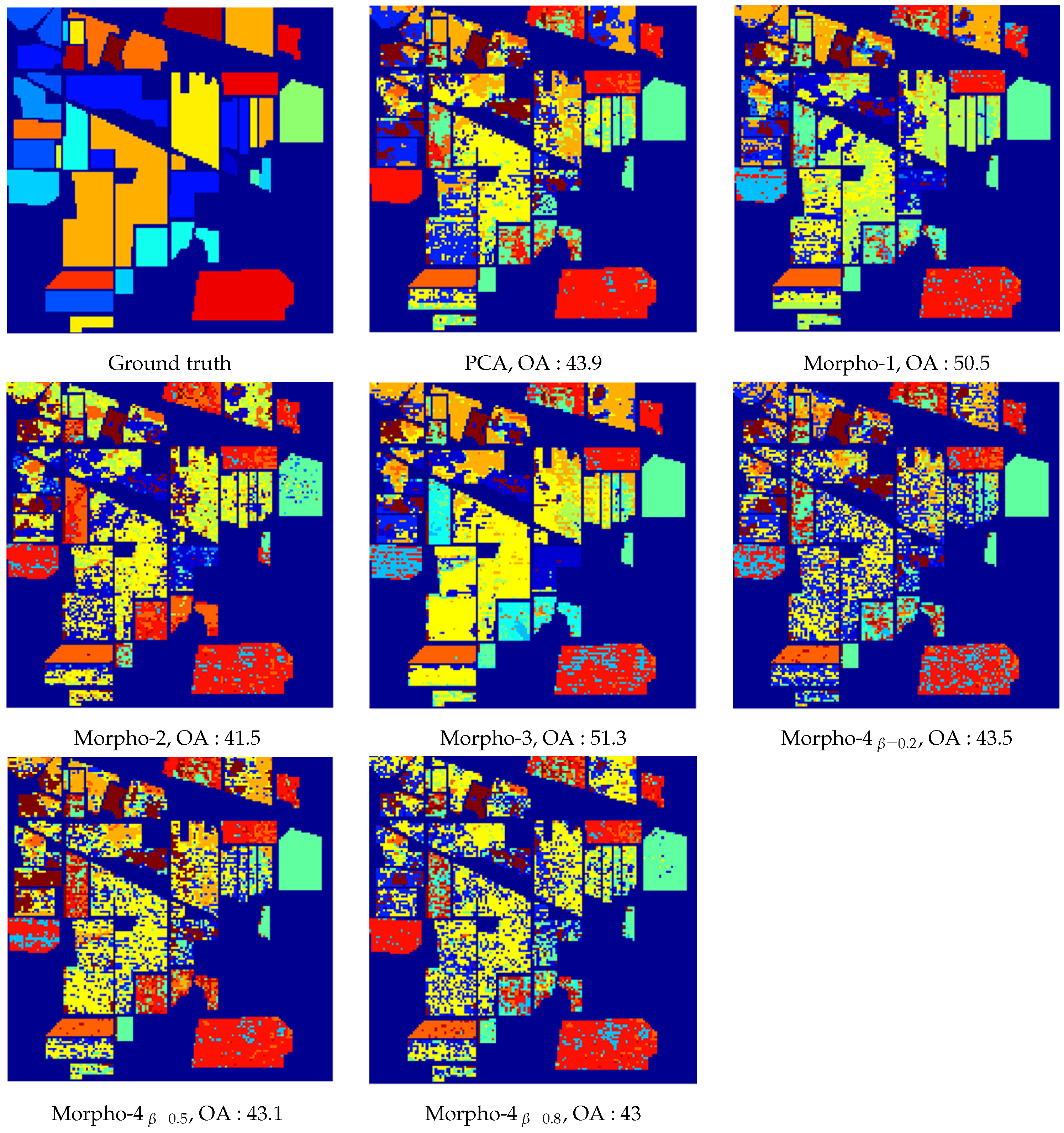
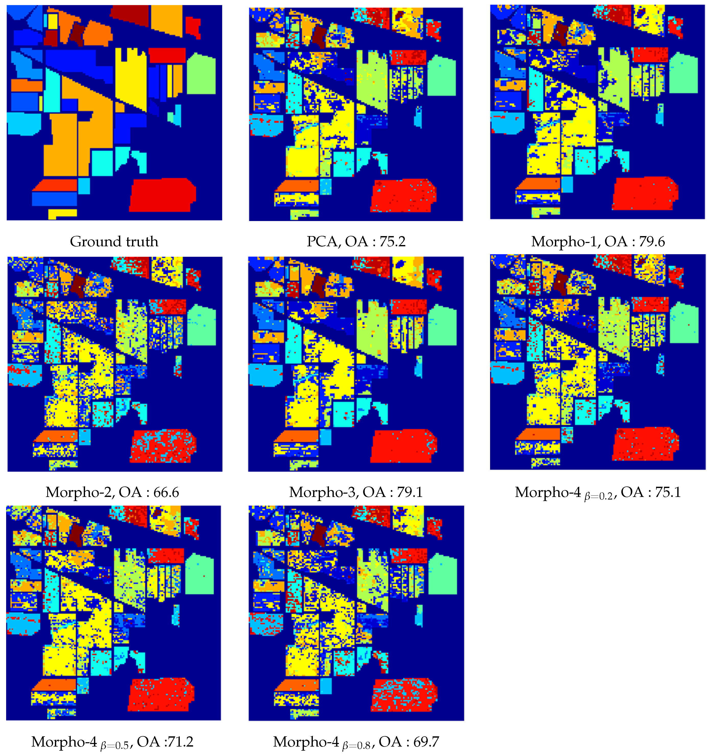
| V | 43.9 ± 3.6 | 75.2 ± 3.7 | 0.73 ± 4.3 × 10⁻⁴ |
| VMorpho-1 | 50.5 ± 3.8 | 79.6 ± 3.7 | 0.78 ± 4 × 10⁻⁴ |
| VMorpho-2 | 41.5 ± 3.8 | 66.6 ± 4.6 | 0.63 ± 4.5 × 10⁻⁴ |
| VMorpho-3 | 51.3 ± 3.2 | 79.1 ± 3.2 | 0.77 ± 3.7 × 10⁻⁴ |
| VMorpho-4 β, β = 0.2 | 43.5 ± 3.3 | 75.1 ± 2.3 | 0.72 ± 2.6 × 10⁻⁴ |
| VMorpho-4 β, β = 0.5 | 43.1 ± 2.9 | 71.2 ± 2.6 | 0.68 ± 3 × 10⁻⁴ |
| VMorpho-4 β, β = 0.8 | 43.0 ± 2.2 | 69.7 ± 3.3 | 0.67 ± 3.9 × 10⁻⁴ |
© 2016 by the authors; licensee MDPI, Basel, Switzerland. This article is an open access article distributed under the terms and conditions of the Creative Commons Attribution (CC-BY) license (http://creativecommons.org/licenses/by/4.0/).
Share and Cite
Franchi, G.; Angulo, J. Morphological Principal Component Analysis for Hyperspectral Image Analysis. ISPRS Int. J. Geo-Inf. 2016, 5, 83. https://doi.org/10.3390/ijgi5060083
Franchi G, Angulo J. Morphological Principal Component Analysis for Hyperspectral Image Analysis. ISPRS International Journal of Geo-Information. 2016; 5(6):83. https://doi.org/10.3390/ijgi5060083
Chicago/Turabian StyleFranchi, Gianni, and Jesús Angulo. 2016. "Morphological Principal Component Analysis for Hyperspectral Image Analysis" ISPRS International Journal of Geo-Information 5, no. 6: 83. https://doi.org/10.3390/ijgi5060083
APA StyleFranchi, G., & Angulo, J. (2016). Morphological Principal Component Analysis for Hyperspectral Image Analysis. ISPRS International Journal of Geo-Information, 5(6), 83. https://doi.org/10.3390/ijgi5060083