An Efficient Parallel Algorithm for Multi-Scale Analysis of Connected Components in Gigapixel Images

Abstract

Differential Morphological Profiles (DMPs) and their generalized Differential Attribute Profiles (DAPs) are spatial signatures used in the classification of earth observation data. The Characteristic-Salience-Leveling (CSL) is a model allowing the compression and storage of the multi-scale information contained in the DMPs and DAPs into raster data layers, used for further analytic purposes. Computing DMPs or DAPs is often constrained by the size of the input data and scene complexity. Addressing very high resolution remote sensing gigascale images, this paper presents a new concurrent algorithm based on the Max-Tree structure that allows the efficient computation of CSL. The algorithm extends the “one-pass” method for computation of DAPs, and delivers an attribute zone segmentation of the underlying trees. The DAP vector field and the set of multi-scale characteristics are computed separately and in a similar fashion to concurrent attribute filters. Experiments on test images of 3.48 to 3.96 Gpixel showed an average computational speed of 59.85 Mpixel per second, or 3.59 Gpixel per minute on a single 2U rack server with 64 opteron cores. The new algorithms could be extended to morphological keypoint detectors capable of handling gigascale images.

1. Introduction

Multi-scale analysis is pivotal in both human and computer vision [1,2,3,4,5,6]. This is in part due to the fact that features of importance might be present at a range of scales, depending on distance to the observer or camera. Conceptually, multi-scale analysis maps the image onto a higher-dimensional space or stack of images. The problem then is to identify the most important or salient features in this scale space [5,7,8].

Multi-scale methods based on connected morphological filters [1,2,9,10,11] of various types have been useful in remote sensing applications, both in multi-band processing and in gray-scale (typically panchromatic) images. In the former case, alpha-trees [12] or other partition hierarchies are used most [13,14], whereas in the latter methods being based on either reconstruction or attribute filters is most common. The most popular of these gray-scale methods are Differential Morphological Profiles (DMPs) [7,8], Differential Area Profiles [15,16], and their generalization Differential Attribute Profiles (DAPs) [17,18].

In this paper, we will focus on these latter gray-scale methods and review recent developments in this field, in particular, adaptation of algorithms for parallel computation of multiscale representations. In addition, we will introduce a number of improvements to existing algorithms, and compare the computational performance and memory load of these methods. A common factor limiting the usability of both DMPs and DAPs is the lack of efficient means for handling the massive input-data size. The memory load and computation-time of standard iterative methods increase linearly with respect to both input image size and the number of scales used [8,16].

DMPs [7,8] are sets of top-hat scale-spaces based on openings by reconstruction. Traditionally, they can be computed by first performing a series of erosions with an increasing set of structuring elements (SEs), computing a geodesic reconstruction from each of these marker images, and finally taking the differences between successive reconstructions, where the reconstruction of the smallest SE is subtracted from the original. Thus, a stack of images is obtained, representing a top-hat scale space, each of which stores bright details of a certain width range, dictated by the widths of the SEs used. To obtain the dark details, a similar process is performed after first inverting the input image. The DMPs have a large spectrum of applications in the field of Earth and planetary science, computer science, engineering, physics and astronomy, and mathematics. In the field of remote sensing, they are mostly applied for the image feature extraction phase and filtering or knowledge-driven image information selection purposes. The output of DMPs is typically used as input of supervised or unsupervised classification processes. The computation of DMPs in the classical way involves multiple reconstruction operations, which is costly. In [8], it was shown that the process could be sped up by (i) using a single Max-Tree [19] to compute all reconstructions in a single pass, and (ii) using parallel processing based on the algorithm in [20].

Differential attribute profiles [15,17,21] are generalizations of DMPs based on connected attribute filters [22]. Instead of a series of openings-by-reconstruction, a series of attribute filters are used which form either a size or shape granulometry [23,24]. Again, differences between consecutive filtered images are taken to create a stack of images containing different size or shape classes of details, and again, this stack of images is usually summarized in a single multi-band image. An example of sets of DAPs in the cross-section of an area opening top hat scale space and an area closing bottom hat scale space is shown in Figure 1.

Applications of DAPs vary and typical examples are scene classification [18,25], image segmentation [26,27], urban pattern characterization [28,29,30,31,32] and human settlement visualization [33]. Note that both the DAP and DMP can be considered alternatively as a set of images at different scales, or as a vector image, in which each pixel is represented by a vector of values corresponding to the response in each morphological filter band.

The CSL is a general model suitable for compact representation of multi-scale image decomposition schema, including DMPs and DAPs. It consists of three raster layers derived from the image multi-scale decomposition; the Characteristic scale (C), the Saliency (S) and the Leveling (L). The basic components of the CSL (C, S) were firstly introduced in [34] supporting a classification schema made with a neural supervised classifier of image connected components (also called regions or objects) and their attributes. Subsequently, they were presented in [7,35] for general image segmentation purposes. In [36], the DMP concept was reintroduced with the name of “ultimate opening” and the same C, S elements of the DMP were presented with the name of parameters of maximal residue v and the size q of the opening leading to this residue. With the latter naming, they have been applied for segmentation of text regions in digital images in [37] and shape recognition tasks in [38]. In [33,39], the CSL schema was completed with the explicit introduction of the leveling (L) descriptor and applied for reduction of the dimensionality and the memory storage/allocation cost of the image multi-scale decomposition. In particular, the need of performing massive unsupervised image processing tasks in a statistical-model-free approach, i.e., avoiding clustering based on the statistical distribution of the DMP/DAP features, was addressed. The image data scale-decomposed and described by the CSL schema can be used for knowledge-driven image information mining and selection [39,40], supervised and unsupervised classification [41,42,43,44] and visualization purposes [39,45].

In the case of DAPs as with DMPs the problems with memory load and compute time can be addressed using Max-Trees, and their dual Min-Trees [19]. One key problem is the need to store the entire scale space, or vector field, consisting of as many images as there are scales. In the DMP case, this is unavoidable, because the marker images are needed for each scale. These markers can be reused to store the DMP vector field itself, as in [8]. In the case of the DAP, this can be avoided if all we need is a summary such as the CSL representation. Extending the work on fast computation of connected granulometries and pattern spectra in [24], in [16], a scheme was proposed that is referred to as the attribute zone decomposition. Tree nodes are assigned a unique zone label depending on the attribute value of the image component they associate with. Organizing the tree nodes into zones requires a single pass through the tree structure and has a minimal dependency on the length of the signature. This scheme is called the one-pass method. A performance comparison against other iterative methods is given in [16].

Apart from zone labeling, the one-pass method can be applied to compute the set of features that constitute the CSL model [33]. The DAP vector field, i.e., the set of DAPs accounting for the entire input image, is extracted by mapping each image component to the respective DAP plane. There are twice as many planes as the number of attribute thresholds defining the decomposition. The model is computed directly from the two tree-based data structures and with no need of exporting the DMP/DAP vector fields.

Building upon a parallel method for computing the Max-Tree structure on shared memory platforms, in this paper, a new concurrent version of the one-pass method is presented. The algorithm is based on the concurrent algorithm for Differential Morphological Profiles [8], which, in turn, was based on the shared-memory parallel algorithm for component trees from [20]. We adapt the existing algorithm for DMP to the DAP, and develop this further to produce an algorithm which does not compute the entire vector field, but just the data needed for the CSL model computation. The latter is both faster and much more memory-efficient. The code can handle images up to 4 Gpixel, the limit imposed by GeoTIFF, and processing on a 64-core machine shows speeds of over 3.5 Gpixel per minute. Extension to larger volumes requires only using 64-bit rather than 32-bit indexing of the arrays used, and, of course, a different input format.

The structure of this paper is as follows. Section 2 gives a brief overview of connected attribute filters, differential attribute profiles and the CSL model. In Section 3, the Max-Tree structure is revisited followed by a brief description of the one-pass method. The proposed concurrent algorithm for computing the DAPs and the CSL bands is presented in Section 4. A set of timing experiments on very high resolution satellite images follows in Section 5. A discussion and analysis of the experimental results is given in Section 6, and a summary of the work presented together with conclusions, in Section 7.

2. Background

2.1. Attribute Filters

Attribute filters [22] are morphological filters designed to preserve or remove connected image structures based on their properties or attributes. These attributes can be anything, ranging from simple size measures such as area [46], through shape numbers [23,24] to feature vectors. In the binary case, they simply remove all connected foreground or background components based on a selection criterion, based on the attribute values, and some decision boundary.

Let E be the definition domain of a gray-scale image $f:E\to \mathbb{R}$, and let the information content of f be organized into a set of flat zones [11], the union of which, equals E. A flat zone F is a connected set of maximal extent. It consists of isotone pixels that are path-wise connected. Given a point $x\in E$, F is formally defined as:

$$F_x\left(f\right)=\left\{x\right\}\cup \{y\in E\mid \exists \pi (x⇝y)\wedge f\left(y\right)=f\left(x\right)\}$$

(1)

in which $\pi (x⇝y)$ denotes a path from x to y. The set of image flat zones constitutes a partition of E. To introduce a notion of order with respect to image intensity a more general type of component is defined. A peak component marked by a point $x\in E$ at level h is given by:

$$P_x^h\left(f\right)=\left\{x\right\}\cup \{y\in E\mid \exists \pi (x⇝y)\wedge f\left(y\right)\ge f\left(x\right)\}$$

(2)

A peak component that coincides with a single flat-zone is called a regional maximum.

Connected filters consider connected operators that access peak components instead of individual pixels. In particular, gray-scale attribute filters [22] are image transforms that reduce the information content by removing peak components that fail an attribute criterion. Attribute filters are idempotent, i.e, re-iterating the operator does not modify the result further. Attribute filters are edge preserving operators and can be categorized based on the intensity order they are configured with, and the properties of the attribute they employ. A filter that treats bright components as foreground information against a dark background is denoted as ${\gamma }_{\lambda }^A$ and is called an attribute opening if the criterion is increasing, or thinning otherwise. By contrast, a filter that treats dark components as foreground information against a bright background is denoted as ${\phi }_{\lambda }^A$ and is called an attribute closing if the criterion is increasing, or thickening otherwise. The term A specifies the attribute type, and λ the attribute threshold.

2.2. Differential Attribute Profiles and the CSL Model

Consider a dual pair of attribute filters $({\gamma }_{\lambda }^A,{\phi }_{\lambda }^A)$ and an attribute threshold vector $\overrightarrow{\lambda }=\left[{\lambda }_i\right]$ with $i\in [0,1,2,\dots ,I-1]$ and ${\lambda }_0=0$. For each filter, let ${\Delta }^{\Pi }$ be a differential profile that is given a point $x\in E$ defined as follows:

$${\Delta }^{\Pi }\left({\gamma }_{\lambda }^A\left(f\right)\right)\left(x\right)=\left(({\gamma }_{{\lambda }_{i-1}}^A\left(f\right)-{\gamma }_{{\lambda }_i}^A\left(f\right))\left(x\right)\mid {\lambda }_i>{\lambda }_{i-1},\forall i\in [1,\dots ,I-1]\right)$$

(3)

for the filter ${\gamma }_{\lambda }^A$, and

$${\Delta }^{\Pi }\left({\phi }_{\lambda }^A\left(f\right)\right)\left(x\right)=\left(-({\phi }_{{\lambda }_{i-1}}^A\left(f\right)-{\phi }_{{\lambda }_i}^A\left(f\right))\left(x\right)\mid {\lambda }_i>{\lambda }_{i-1},\forall i\in [1,\dots ,I-1]\right)$$

(4)

for ${\phi }_{\lambda }^A$. Each profile is a response vector associated to x. ${\Delta }^{\Pi }\left({\gamma }_{\lambda }^A\right)$ is called the positive, and ${\Delta }^{\Pi }\left({\phi }_{\lambda }^A\right)$ the negative response vector respectively. The concatenation of the two, denoted with ⊔, is a $2\times (I-1)$ long vector, called the differential attribute profile [17] of x:

$$\text{DAP}\left(x\right)=({\Delta }^{\Pi }\left({\gamma }_{\lambda }^A\left(f\right)\right)\bigsqcup {\Delta }^{\Pi }\left({\phi }_{\lambda }^A\left(f\right)\right))\left(x\right)$$

(5)

The set of DAPs computed from the full extent of image definition domain is called the DAP vector field. An instance i of a DAP vector field is a different image with respect to the given operator and is called a DAP plane. Figure 2 shows an example. Image (a) shows a residential section of the city of Sana’a, Yemen. It is a 2009, Quickbird panchromatic image ©DigitalGlobe, Inc., at 0.6m spatial resolution in colormap projection. Image (b) shows the DAP vector field computed from (a). The visualization in (b) employs 3D connected component color labels. The top volume set in (b) shows the area opening top-hat scale-space and the lower volume set shows the area closing bottom-hat scale space.

The extreme values of an entry in any of the two response vectors are 0 and $h_{\text{max}}$ with the latter being the maximal image intensity value. Consider a point $x\in E$ and let ${\check{dh}}_{{\gamma }_{\lambda }^{\Lambda }}$ be the highest value in the positive response vector of DAP$\left(x\right)$, i.e.,:

$${\check{dh}}_{{\gamma }_{\lambda }^{\Lambda }}\left(x\right)=\vee {\Delta }^{\Pi }\left({\gamma }_{\lambda }^{\Lambda }\right(f\left)\right)\left(x\right)$$

(6)

which is given at a scale i. Note that i may not be necessarily unique, i.e., the same response can be observed at other scales too. However, since the most relevant information of the decomposition are contained within planes associated with smaller scales, the parameter:

$${\widehat{i}}_{{\gamma }_{\lambda }^{\Lambda }}\left(x\right)=\wedge i:({\gamma }_{{\lambda }_{i-1}}^{\Lambda }-{\gamma }_{{\lambda }_i}^{\Lambda })\left(x\right)={\check{dh}}_{{\gamma }_{\lambda }^{\Lambda }}\left(x\right)$$

(7)

is identified. That is, ${\widehat{i}}_{{\gamma }_{\lambda }^{\Lambda }}$ is the smallest scale at which the positive response vector of the $\text{DAP}\left(x\right)$ registers the maximal response. The equivalent scale parameter for the negative response vector is defined analogously:

$${\widehat{i}}_{{\phi }_{\lambda }^{\Lambda }}\left(x\right)=\wedge i:({\phi }_{{\lambda }_i}^{\Lambda }-{\phi }_{{\lambda }_{i-1}}^{\Lambda })\left(x\right)={\check{dh}}_{{\phi }_{\lambda }^{\Lambda }}\left(x\right)$$

(8)

They are referred to as the multi-scale opening and closing characteristic, respectively; MOC and MCC.

Consider the following labeling scheme based on the maxima of the two response vectors:

• convex, if ${\check{dh}}_{{\gamma }_{\lambda }^{\Lambda }}\left(x\right)>{\check{dh}}_{{\phi }_{\lambda }^{\Lambda }}\left(x\right)$,
• concave, if ${\check{dh}}_{{\gamma }_{\lambda }^{\Lambda }}\left(x\right)<{\check{dh}}_{{\phi }_{\lambda }^{\Lambda }}\left(x\right)$,
• flat, if ${\check{dh}}_{{\gamma }_{\lambda }^{\Lambda }}\left(x\right)={\check{dh}}_{{\phi }_{\lambda }^{\Lambda }}\left(x\right)$.

This is the equivalent taxonomy to the ones proposed based on the differential morphological and area profile decompositions in [7] and [16] respectively. The set of labels is referred to as the local curvature of the gray level function surface, where the attribute value determines the local spatial domain.

An intuitive multi-band segmentation scheme is then:

$$\overline{i}\left(x\right)=\{\begin{array}{}\mathrm{(9a)}& {\widehat{i}}_{{\gamma }_{\lambda }^{\Lambda }}& & \text{if convex},\mathrm{(9b)}& {\widehat{i}}_{{\phi }_{\lambda }^{\Lambda }}& & \text{if concave},\mathrm{(9c)}& 0& & \text{if flat}.\end{array}$$

This multi-level segmentation scheme can be further simplified to a three-band segmentation by replacing the scale parameter with a fixed gray-level.

The winning scale from the comparison in Equation (9) is referred to as the characteristic scale or simply characteristic C. The response associated with the winning scale is called the saliency S and is denoted by $d\overline{h}$. The two, complemented by the level L of the pixel x after the iteration of the respective attribute filter at the reference scale i, denoted as ħ, constitute the three bands of the CSL model [33]. The latter is a non-linear mixture model used for compact representation of multi-scale image information to be used for classification and other analytic purpose. An example of CSL used for visualization purposes is shown in Figure 2c; computed from a.

2.3. Attribute Zone Decomposition

Attribute filters acting on a gray-scale image produce a dichotomy, i.e., they separate the image contents in two sets of components—those that satisfy the attribute criterion and those that fail it. Extending this for multiple attribute thresholds gives rise to the concept of attribute zone decomposition. Each zone is a grouping of peak components with attribute values being within some prespecified range.

Let ${\Gamma }_{\lambda }^{\Lambda }$ and ${\Phi }_{\lambda }^{\Lambda }$ be the binary counterparts of ${\gamma }_{\lambda }^{\Lambda }$ and ${\phi }_{\lambda }^{\Lambda }$ respectively, and consider a threshold decomposition of f [47]. Each threshold set $T_h\left(f\right)$, with $h\in \{h_{min},\dots ,h_{max}\}$, contains $k\in K_h^f$ peak components $P_k^h$, and for each pixel $x\in E$ the characteristic function χ of $T_h\left(f\right)$ is given by:

$$\left(\chi \left(T_h\left(f\right)\right)\right)\left(x\right)=\left\{\begin{array}{cc}\hfill 1& \text{if}x\in T_h\left(f\right),\hfill \\ \hfill 0& \text{otherwise}.\hfill \end{array}\right.$$

(10)

Definition 1. 

The attribute zone ${\zeta }_{{\lambda }_a,{\lambda }_b}^A$ of a mapping $f:E\to \mathbb{Z}$, bounded by two attribute thresholds ${\lambda }_a$ and ${\lambda }_b$ such that ${\lambda }_a<{\lambda }_b$, is given by:

$${\zeta }_{{\lambda }_a,{\lambda }_b}^A\left(f\right)={\displaystyle \sum _{h=h_{\text{min}}+1}^{h_{\text{max}}}}\left({\displaystyle \sum _{k\in K_h^f}}\chi \left({\Gamma }_{{\lambda }_a}^A\left(P_k^h\right)\backslash {\Gamma }_{{\lambda }_b}^A\left(P_k^h\right)\right)\right)$$

(11)

In brief, the intensity of any point x of the image domain, that marks a component in a zone ${\zeta }_{{\lambda }_a,{\lambda }_b}^A$ can be obtained by initializing it to zero and updating it by adding the value of 1 for each level at which, $x\in P_k^h$ is non-zero in the difference between the two attribute filters ${\Gamma }_{{\lambda }_a}^A$, ${\Gamma }_{{\lambda }_b}^A$. The same decomposition is defined for the operator ${\Phi }_{\lambda }^A$. The attribute zone operator is a connected operator and it generates an attribute-based decomposition as described in [16], i.e., any two zones do not overlap and the decomposition is unique.

2.4. The DMP vs. the DAP

The DMP is a special case of a DAP, just as reconstruction filters are a special case of attribute filters. By replacing the general attribute filters in the DAP by reconstructions from a set of markers, we obtain the DMP. The set of markers replaces the set of attribute thresholds, and this is where there is an important difference in terms of computation, as will be discussed in the following sections. The key point is that the markers themselves need to be stored in memory as a stack of images. As has been shown [8], we can reuse this space to store first the stack of reconstructed images, and finally, the output DMP. The latter can then be processed into an MOC or MCC. Though the algorithm in [8] is highly efficient, we will explore a one-pass method and further economies to increase the performance further.

3. The Max-Tree Algorithm and the One-Pass Method

An efficient method for computing the DAP vector field and the CSL model has been presented in [16]. It relies on a combination of the Max-Tree and Min-Tree image representation structures [19] for computing the attribute zone decomposition discussed in the previous section.

The Max-Tree of an image f is a tree for which the node hierarchy corresponds to the nesting of the peak components of f. Each node $N_k^h$ is addressed by its level h and its index k, and corresponds to a set of flat-zones [11] for which there exists a unique mapping to a single peak component:

$$N_k^h=\{x\in P_k^h\mid f\left(x\right)=h\}$$

(12)

The “leaves” of the tree correspond to the regional maxima of f and its root is defined at the lowest gray level of the structure, representing the set of background pixels.

In the current implementation, as in [20], each pixel is represented by a Max-Tree node, stored in an array of the same size as the image. All nodes contain a parent reference, represented as a 32-bit unsigned integer. A boolean field valid indicates whether a node has been processed or not. In the general case of attribute filters, each node contains a pointer to a set of auxiliary attribute variables that are updated from its member pixels during the construction of the tree [48]. In the case of area filters, memory is saved by using an area field, also represented as a 32-bit unsigned integer instead. A peak component’s area is computed by summing the area of its descendants with the total area of its flat-zones. Within each peak component, a single pixel is chosen as the representative, or canonical element. We call this pixel the level root. All pixels of a peak component, except the level root point to the level root. The level root itself points to a pixel in the parent peak component. The root of the tree points to a global root ⊥.

The Max-Tree is computed using a hierarchical, depth-first, flood-filling algorithm introduced by Salembier et al. [19]. Alternative methods were presented in [49,50,51,52]. The recursive method discussed in [19] separates the construction of the tree from the computation of attributes and the actual filtering. This architecture is particularly appreciated in applications requiring interactive filtering or multiple filtering instances. Note that the Min-Tree is an equivalent representation to the Max-Tree of the inverted input image.

The one-pass method for computing the attribute zones on each of the two trees was presented in [16]. A pseudo-code listing can be found in the same article. The methods follows a similar approach to the filtering functions described in [19,48]. Attribute zones are independent of the various root-paths and they are identified by a unique integer corresponding to the zone’s ${\lambda }_b$ address in the $\overrightarrow{\lambda }$ vector:

$$\text{ZoneID}\left(P_k^h\right)=\wedge \left\{i\in \{1,\dots ,I-1\}\mid Attr\left(P_k^h\right)<{\lambda }_i\right\}$$

(13)

In words, the zone ID member of each node is set to the address of the lowest attribute threshold from $\overrightarrow{\lambda }$ for which the peak component under study fails the attribute criterion. Once the image is decomposed into its attribute zones, the two instances of the DAP field each of which is an (I − 1) × ImageSize volume set, can be extracted by visiting each pixel I − 1 times, i.e., once for each area zone.

4. A Concurrent One-Pass Method

In this section, we study how the above approach can be adapted for the concurrent computation of the Differential Attribute Profile. We first focus on the case of increasing attributes, and, in particular, the case that the attribute is the area of each component. Two cases can be separated: (i) explicit computation of the DAP vector field, and (ii) direct computation of the MOC, and, by duality, the MCC.

4.1. Parallel DAP Computation

Unlike the DMP, we do not have to compute any marker images. We simply need a Max-Tree with suitable attributes computed for all nodes. We do need an array out of numscales images to store the output. An array lambda containing the scale-class boundaries is required as input. Rather than filtering the image at each level explicitly, and computing the difference at consecutive scales, we approach the problem in a similar way to that in [8]. A single filtering stage computes the entire DAP. The algorithm is shown in Algorithm 1.

Each process or thread p scans the section V^p assigned to it. Any pixel for which the corresponding node has not yet been marked as valid is processed. Starting at the smallest scale, the algorithm follows the root path until it either finds the global root, or a valid node, or it finds a node with an area larger than the current scale. It does this for all scales, storing the node location in an array ws, and the corresponding gray level in an array val. After all scales are processed, a second pass along the root path is made, setting all values in the DAP array out to the correct values for all pixels in its section V_p.

After this pass, each slice of the array out contains the area opening for the appropriate scale λ_i represented in the pseudo code by lambda [i]. What remains is to compute the differences between successive slices to obtain the final DAP.

The disadvantage of this approach is that both memory use and computational time scale linearly with the number of scales. This becomes prohibitive for large numbers of scales.

4.2. Direct MOC Computation

Like the previous algorithm, we assume that the Max-Tree has been computed with all attribute information in place. Computing the MOC directly can be done without the need for storing a DAP vector field. Instead, we only compute the supremum of the DAP vector for each scale, stored in image outDH, along with a relevant scale, stored in image outScale, and the orginal gray level at that scale for each pixel in the image, stored in image outOrig. To compute this, we equip each Max-Tree node with fields maxDH and scale both of gray-level type (unsigned char in our case). As before, array lambda stores the scale class boundaries.

Algorithm 1 The filtering stage of the parallel Differential Attribute Profiles (DAP) algorithm

procedure MaxTreeMakeDAP (Vp : Section; var node : Max-Tree; var out : DAP; lambda : integer[numscales]) for all v ∈ Vp do if not node[v].valid then w := v; for all scales i increasing order do while Par(w) ≠ ⊥ ⋀ not node[w].valid ⋀ node[w].area < lambda[i] do w := Par(w); end; ws[i] := w; (∗ temporary storage of for each scale ∗) if node[w].valid then for all scales j ≥ i do (∗ filtered node found ∗) val [j] := out[j][w]; end; else if node[w].area ≥ lambda[i] then (∗ w is filtered ∗) val[i] := out[i][w]; else (∗lambda[i] too large ∗) val[j] := 0; end; end; end; end; u := v; for all scales i increasing order do repeat if u ∈ Vp then for all scales j < i do out[j][u] := f [u]; end; for all scales j ≥ i do out[j][u] := val[j]; end; node[u].valid := true; end; u := node[u].parent; until u = ws[i]; end; if u ∈ Vp then (∗ Process ws[numscales − 1] ∗) for all scales j < i do out[j][u] := f [u]; end; node[u].valid := true; end; end; end;

In a first version of the algorithm, we reused the area field to store the scale class (as an integer). This algorithm worked in two stages (after building the tree). In the first stage, we simply compute the scale class for each level root in the tree. This can be done completely in parallel, because the decision is local. After this, the tree was traversed in much the same way as the original one-pass method.

Some initial experiments showed that the first phase of this two pass approach was surprisingly inefficient in terms of speed-up, achieving only 16–18 times faster computation on 64 nodes. The reason for this is most likely that it is a very short phase with barriers on either side. This means that load imbalance and synchronization costs have a large impact. We therefore implemented a one-pass version. Here, we do need to introduce a scale field in the tree, and though this is of course more costly in terms of memory, it has an important advantage, in that the area data is not overwritten. This means that we can recompute MOCs with different parameter settings from the same tree, should we need to.

The one-pass algorithm for the MOC computation is given in Algorithm 2, and Algorithm 3. The latter simply scans the section of the image assigned to the process, and calls procedure NodeSetMOC from Algorithm 2 for each node that is not yet valid. This checks if the current node is a level root, and if so, computes the scale and gray level contrast with its parent. Next, it checks whether the scale is maximal, indicating that the current node has area outside the range of interest, and its MOC parameters are set to “out-of-bounds” conditions. No further ascent is needed as all ancestors must have larger areas.

Algorithm 2 The filtering stages of the parallel multi-scale opening characteristic (MOC)

procedure NodeSetMOC (Vp : Section; var node : Max-Tree; current : integer; var maxDH, curScale : grayval; var outDH, outScale, outOrig : array[0, ..., N − 1]of pixel, lambda : integer[numscales] ); var scale, DH : grayval; if IsLevelRoot(node[current]) then (∗ compute scale and DH for current nodes ∗) scale := FindScale(node[current], lambda); DH := getDH(node[current]); end; if IsLevelRoot(node[current]) and scale = numscales then (∗ Initialize to out of scale range ∗) maxScale := numscales; maxDH := 0; curDH := 0; maxOrig := 0; curScale := numscales; else parent = node[current].parent; if not node[parent].valid then (∗ go into recursion to set parent values correctly ∗) NodeSetMOC(Vp, node, parent, maxDH, curScale, outDH, outScale, outOrig, lambda); else (∗ if the parent is valid, copy relevant values ∗) maxScale := outScale[parent]; maxDH := outDH[parent]; maxOrig := outOrig[parent]; curScale := node[parent].scale; curDH := node[parent].curDH; end if IsLevelRoot(node[current]) then (∗ if I have a level root, some things might change ∗) if scale = curScale then (∗ same scale class: add current pixel’s curDH ∗) curDH = curDH + curDH; else (∗ scale class change, update current scale and DH ∗) curDH = DH; curScale = scale; end; if curDH ≥ maxDH then (∗ If updated curDH is higher than or equal to the maximum DH found update maxDH, maxScale, and outOrig ∗) maxDH := curDH; maxScale := scale; outOrig = gval [current]; end; end; end; if current ∈ Vp then (∗ Store the information ∗) outScale[current] := maxScale; outDH[current] := maxDH; outOrig[current] := maxOrig; node[current].scale := curScale; node[current].curDH := curDH; node[current].valid := true end; end;

Algorithm 3 The final filtering stage of the parallel MOC

procedure MaxTreeComputeMOC (Vp : Section; var outDH, outScale, outOrig : array[0, ..., N − 1]of pixel, lambda : integer[numscales] ); var curScale, maxScale, maxDH, curDH, maxOrig : grayval; for all v ∈ Vp do if not node[v].valid then NodeSetMOC(Vp, v, curDH, maxDH, maxScale, maxOrig, curScale, outDH, outScale, outOrig, lambda); end; end; end;

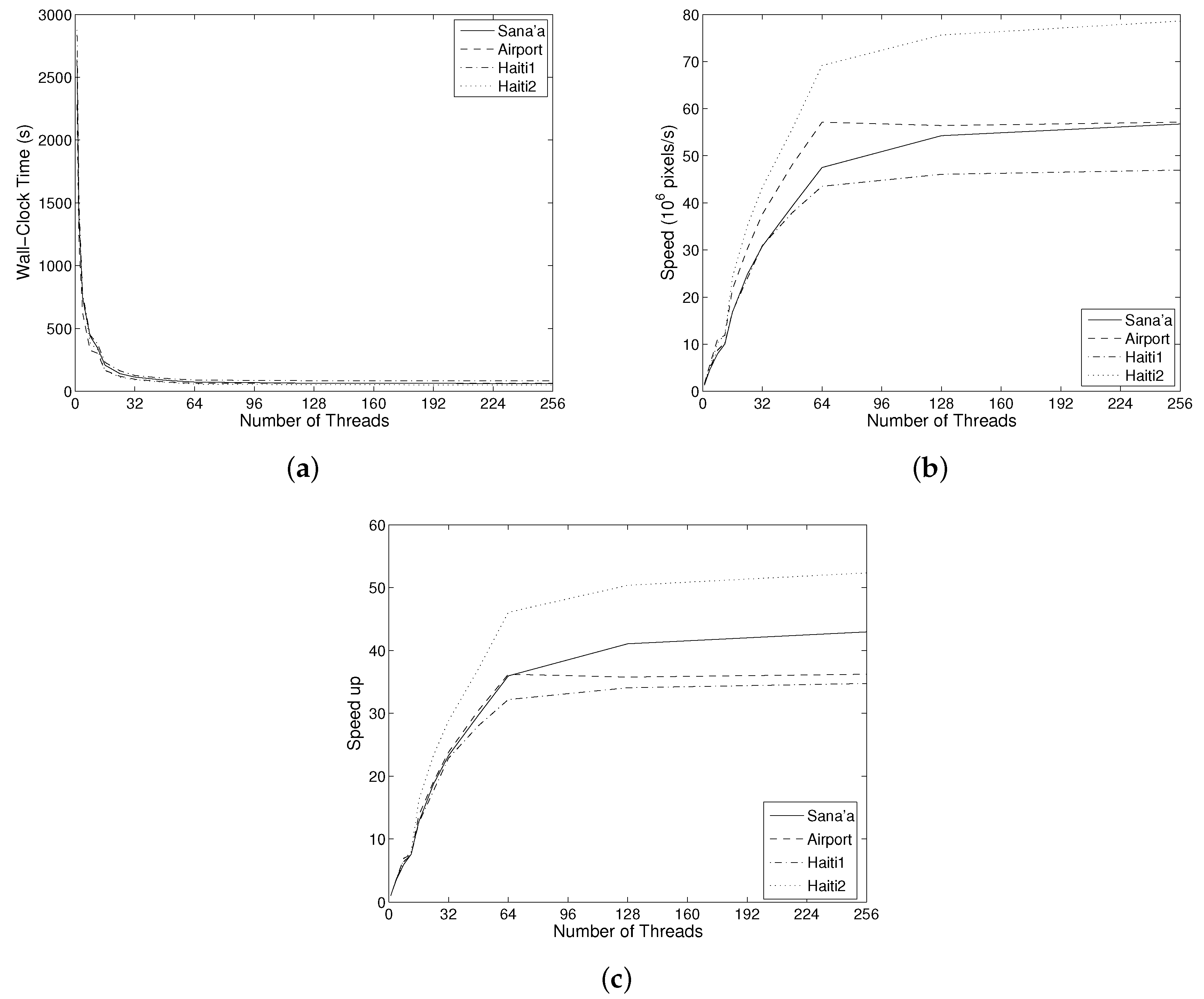
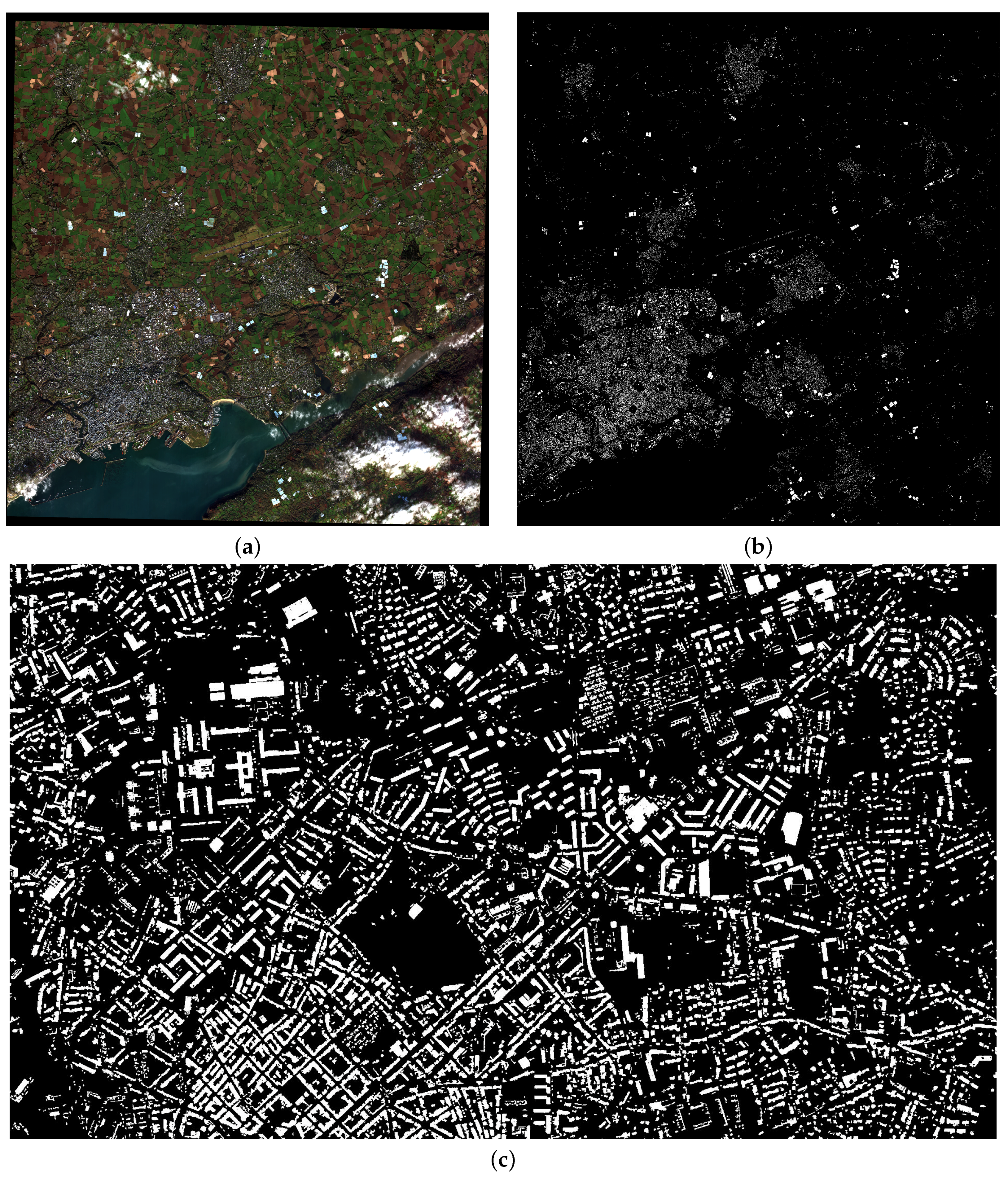
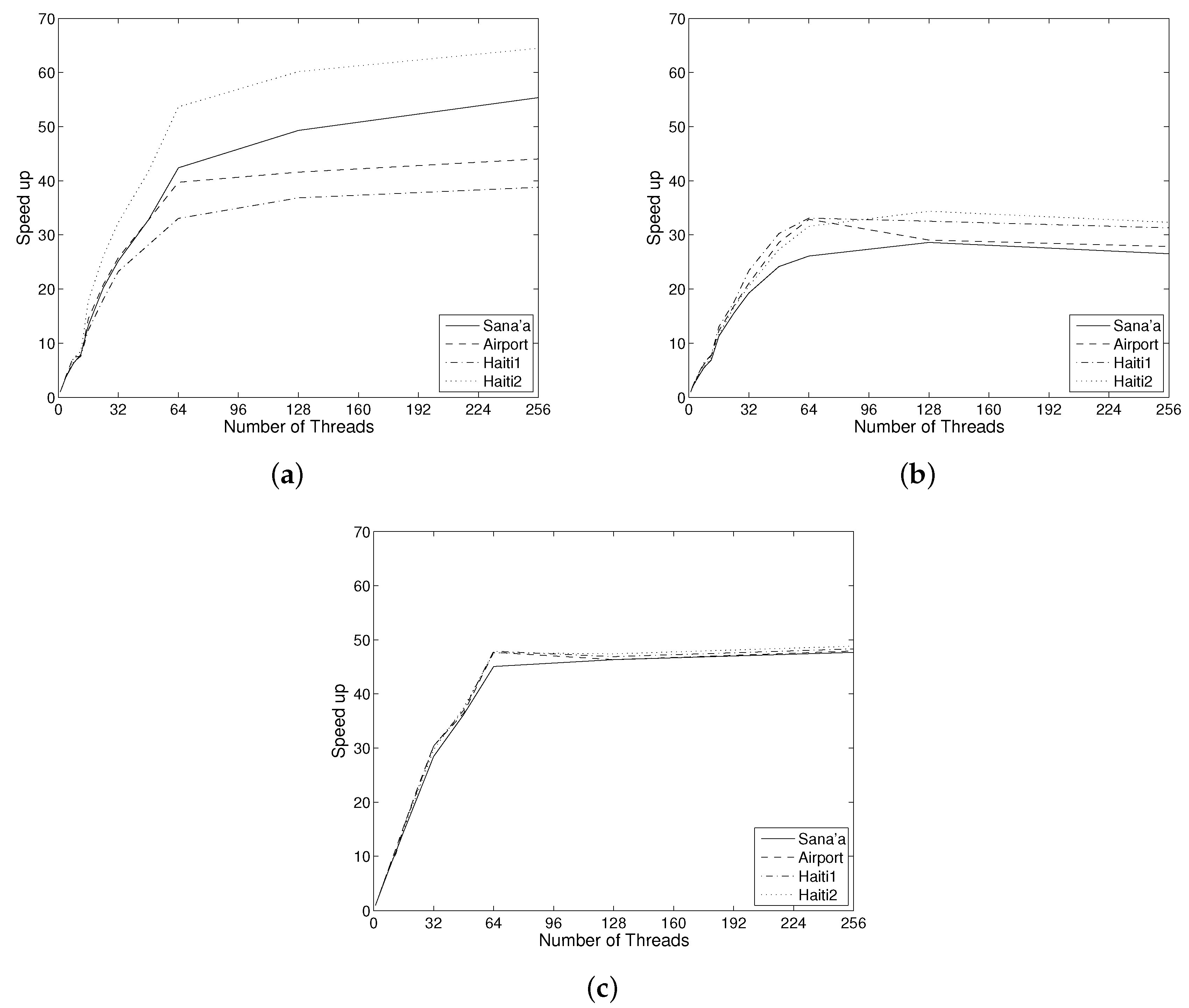
Otherwise, we look up the parent, and check if it is valid or not. If not, NodeSetMOC is called recursively for the parent. Otherwise, the parent data are copied (as they are valid). We now have the correct MOC values of the root path up to the parent of the current node. If the current node is a level root, we check whether its scale is the same as the parent’s value stored in curScale. If so, the contrast value curDH must be incremented with the contrast of the current node, stored in DH. If the scales are not the same, the current scale and contrast are updated to those of the current node.

After this, we check whether the current contrast curDH is larger than or equal to the maximum contrast maxDHm, and if so, maxDH, maxScale, and outOrig are updated (corresponding to the C, S, and L parts of the MOC, respectively).

Finally, if the current node is in the processor private section Vp of the image, the parameters are written to the fields in the node, and to the output MOC. This approach does mean scale values may be computed multiple times by different threads, but this is outweighed by the fact that we lose a barrier.

5. Experiments

The algorithm was implemented in C, and tested on a Dell R815 compute server with 4 Opteron processors with 16 cores each. A total of 512 GB RAM was installed. The source code is available at http://www.cs.rug.nl/~michael/ParMaxTree/. The data sets consisted of a panchromatic Quickbird image of Sana’a, Yemen, courtesy of DigitalGlobe, Inc., two panchromatic post-earthquake images of Haiti, courtesy of Google, and one panchromatic satellite image of an airport. All images were duplicated and tiled to achieve a total image size of between 3.4 and 3.9 Gpixel. For the image properties, see

Table 1. Images used, with size and mean and standard deviation of the gray levels.

Name	Size (× 106 Pixels)	Mean	Std. Dev.
Sana’a	3482	121.78	75.57
Airport	3600	96.58	47.55
Haiti1	3888	107.71	62.99
Haiti2	3963	81.34	52.39

.

5.1. Concurrent CSL Computation

In all cases, timings were performed at 1, 2, 4, 8, 12, 16, 24, 32, 48, 64, 128 and 256 threads. In previous work, we had observed that the Max-Tree building phase could actually speed up further if more threads than cores were used, due to reduced cache thrashing [20]. As the CSL computation was expected to be dominated by the tree-building phase, we wanted to know the impact of this effect.

In the CSL case the final program has the following structure:

(1)

Read image, and create inverted copy of image

(2)

Build Max-Tree from original image

(3)

Compute MOC

(4)

Build Min-Tree from inverted image

(5)

Build MCC

(6)

Combine MOC and MCC to final CSL

(7)

Write output

The parallel CSL-model segmentation program was run 24 times per timing, and the shortest time was considered indicative of the performance of the algorithm in the absence of interference by other programs. In the timing results, we added the Min-Tree and Max-Tree times into one tree-building timing, and likewise for the MOC and MCC times.

Experiments were run in three parameter settings used in practical cases. Two settings with a maximum scale of 16.7 × 10⁶ m² were used, with 12 and 32 scales respectively. The last setting had 64 scales and a maximum area scale of 16, 384 m². It turned out that these settings have no significant impact on the performance of the algorithms. In the following, we discuss the latter timings, with the maximum number of scales.

Figure 3 shows the performance of the algorithm in terms of wall-clock time, speed in millions of pixels per second, and speed up. Total computing times varied from an average of 2609 s at 1 thread, down to 70.8 s at 64 threads, and a further reduction to 64.4 s at 256. The latter is due to reduced cache thrashing during the Max-Tree construction phase [20]. The mean speed up for the complete process is 36.85 at 64 threads, and 40.51 at 256 threads.

Figure 3b shows the computational speed in millions of pixels per second. This calibrates for the differences in processing time due to differences in image size. Despite this correction, quite significant differences are seen. At maximum performance, the processing speed varies from 46.96 Mpixel/s to 78.58 Mpixel/s, with an average of 59.85 Mpixels/s, whereas speed-up varies from 34.74 to 52.36. These differences stem mainly from different complexities of the image. Haiti1 contains only built-up areas, which means that the Max-Tree contains many more nodes. Haiti2 contains large sections of rural area, and some extensive black regions where no data were available. This simplifies the Max-Tree. The Sana’a and Airport images are more mixed.

Construction of the Max-Tree took the most time, using the algorithm from [20], from a mean of 1912 s at a single thread, down to 46.4 s at 64 threads, and further down to 38.8 s at 256 threads. The MOC-MCC phase took 576.75 s on a single thread on average, down to 18.7 s at 64 threads, rising to 21.0 s at 256 threads. Combining the MOC and MCC information into the final CSL-model segmentation is the cheapest by far, costing 105.7 s on one core on average, dropping to 2.25 s on average for 64 cores, with no significant changes beyond.

There are striking differences in speedup between the phases, as seen in Figure 4. The building phase has the highest speed-up on average, but also the largest variation, ranging from 33.05 for Haiti1, to 53.67 for Haiti2 at 64 threads, with an average of 42.22. Beyond 64 threads, there is a further increase in speed up, and 256 threads the speed-up varies from 38.80 for Haiti1 to 64.49 for Haiti2, with an average of 50.67.

The mean speed-up of the MOC-MCC phase is a lot lower, achieving 30.92 on average at 64 threads, with no significant increase beyond that. The final phase has a very good speed up, averaging 47.07 at 64 threads.

By comparison, running the parallel algorithm for differential morphological profiles on the 3.8 Gpixel Sana’a image, using just seven scales, on the same machine, and on a single core, the wall clock time was 5 h 9 min 6.7 s, dropping to 8 min 33.7 s, or a speed up of 36.1, on 64 cores. About half of the wall-clock time is taken up by computation of markers, which is done by computing erosions by exact Euclidean discs by the algorithm of [53]. When using square SE with the same algorithm, the memory use goes down dramatically, and the wall clock time for 7 scales drops to 4 h 10 min 46.8 s and 6 min 19.5 s for 64 cores, or a speed up of 39.6.

The CSL-model segmentation algorithm has a memory complexity of O(N + N_s), with N the number of pixels, and N_s the number of scales. Because N_s << N this becomes O(N) in practice. What we observe is that maximum memory allocation is 24 times the size of the image data, at least for the area attribute. Other attributes would require more memory, as would the use of 64-bit integers for area computation and pixel addressing, as required when going beyond 4 Gpixel images. In that case, we would require 32 times the data size.

By contrast, computing the CSL-model segmentation from the DAP explicitly has a memory complexity of O(N N_s), which becomes prohibitive for large N_s. In the 64 scale case above, the memory usage would rise to 164 times the size of the image (because two arrays of the size of 64N need to be stored). We ran a few experiments on small images, which indicated that computation of the DAP vector field at 64 scales is more than 10 times slower than CSL-model segmentation. On the 870 Mpixel original Sana’a image, the DAP computation took 177.25 s on 64 threads, as opposed to 15.42 s using direct CSL-model segmentation. Even for 12 scales, the difference is factor of two to three. In the case of the 870 Mpixel Sana’a image, the DAP computation took 39.61 s, whereas the CSL-model segmentation took 15.43 s.

For the DMP, the situation is similar to that of explicit DAP computation in terms of memory use. A stack of N_s images is first used to store the markers. These markers are then transformed into reconstructed images, after which pixel-wise differencing is used to obtain the DMP vector field (stored in the same location). This DMP field must then be transformed into a final CSL segmentation. The computational load is typically higher, due to the need for N_s erosions, each of at least O(N) yielding O(N N_s) time complexity. If rotation invariance is needed, this readily increases to O(N N_sR_max) time complexity, with R_max the maximum radius of the SEs used. This initial phase is much more costly than using area as attribute in the DAP, which has constant time complexity per pixel. For more complicated attributes than area, memory load does increase. When using higher order moments the storage per maxtree node goes up roughly as O(M²), with M the order of the moment used, and the compute time increases similarly. As the number of nodes can equal the number of pixels the worst-case memory complexity of the explicit DAP computation becomes O(N(N_s + M²)). For direct CSL computation, it becomes O(N M²), so again, the dependency on the number of scales is removed.

To indicate the severity of the problem, it should be noted that even though our server was fitted with the maximum of 512 GB of RAM, the large data sets could not be run at 64 scales due to memory limitations.

6. Discussion

The results show that parallel computation of CSL-model segmentation can be done very efficiently using the proposed algorithm. We obtain an overall average speed of nearly 60 Mpixel per second, or 3.59 Gpixel per minute, even for 64 scales in the CSL-model segmentation. This means that routine processing of these very large images becomes possible on fairly standard computing servers as well as high-end workstations. Furthermore, if the Max-Tree is built once, it could be stored, and different CSL-model segmentations could be made with different scale parameters. For images of the sizes used here, this would take between 14.09 and 26.62 s. Whilst this is not exactly a real-time response, it is tolerably fast. These later phases of the algorithm have linear time complexity, and for the original Sana’a image (870 Mpixel) the MOC-MCC and CSL-model segmentation phases can take as little as 3.90 s (out of a total compute time of 15.49 s).

It is curious that the MOC-MCC phase of the algorithm has the least speed up, and seems to be limited to about 32. We considered whether this might be due to the fact that some floating point math was used in this phase. The R815 server may have 64 cores, but these share only 32 floating point units between them. We replaced the floating point code with integer math but obtained only a slight speed increase. Therefore, we surmised that the fact that area scales of a given node might be computed multiple times is the problem. However, an earlier version computed the area scale for each node in parallel, and then used the results in a slightly simpler MOC-MCC phase. In this case, the MOC-MCC-phase was no faster: 20.37 s for the 3.48 Gpixel Sana’a image, vs. 20.22 s, when area scales are included in the MOC-MCC phase. This difference is not significant, suggesting that this is not the solution. By putting the scale computation inside the MOC-MCC phase, a barrier was removed, and the overall performance increased a great deal. For the 3.48 Gpixel Sana’a image, the wall-clock time at 256 threads dropped from 73.11 s to 61.37 s.

It therefore seems reasonable that the main cost lies in having to traverse the Max-Tree in parallel, with multiple threads traversing the same root-paths several times. Adding extra computations per node visited has only a very minor impact on either wall-clock time or speed-up. Thus, we find that the fairly complex MOC-MCC phase costs only little more than a single filtering stage of an area opening. This has large implications for the speed gained by the proposed algorithm, quite apart from the parallelism gained.

By comparison, performing a single area filter step on a precomputed Max-Tree of these large images takes roughly 3–5 s, depending mainly on image content. For 64 scales, this would mean 128 filter steps, which comes to a value between 384 and 640 s, assuming no slow-down due to synchronization issues. With the new algorithm, this range is roughly 14 to 27 s (some 25 times faster) regardless of the number of scales.

A variant of this parallelization strategy for the Max-Tree algorithm and the CSL computation is hosted in DigitalGlobe’s Geo Spatial Big Data platform (GBDX) (http://www.digitalglobe.com/) for computing the raw CSL layers of each queued image prior to radiometric classification. This is a building foot-print extraction service operated in the cloud which can be optimized to process all of DigitalGlobe’s WorldView two and three multispectral imagery in near real time. The respective workflow computes the CSL triplet that is configured to contain the most relevant/descriptive image structures compared to the full DAP vector field. These in turn, can be classified efficiently using radiometric features at a meta-process stage and have possible noise elements removed. Efficiency in this case comes as a consequence of reduced number of test samples (dominant CSL structures). An example is shown in Figure 5. Image (a) shows an RGB view of an eight-band multi-spectral data-set covering the city of Brest, France and its surroundings. This is a WorldView 2 image © DigitalGlobe, Inc (Westminster, CO, USA), at 1.6 m. spatial resolution following ortho-rectification and atmospheric compensation (14 bpp data-depth). The image was acquired on 15 October 2014 and covers a total area of 313 km². Image (b) shows the respective CSL-segmentation following natural element refinement procedures. The segmentation targets all built-up structures independent of size, structural or radiometric characteristics. Image (c) shows a zoom-in view of the city’s center north of its port. This workflow makes use of MOCs only (i.e., a Max-Tree structure alone) thanks to a novel band blending method reducing WorldView 2 or 3, 8-band atmospherically compensated data-sets to gray-scale layers that show a strong response to building materials exclusively.

7. Conclusions

In this paper, we have presented a new algorithm for efficient, shared memory, parallel computation of the CSL-model segmentation and CSL profile of images in the gigapixel range, besides several improvements on existing DMP, Multi-Scale Leveling Segmentation (MSLS), and DAP algorithms. The CSL algorithm can be adapted to any increasing attribute, by incorporating the auxiliary data handling described in [20]. One such extension to 2D pattern spectra has already been provided, using area and non-compactness as attributes [54]. More complicated attributes will impact on Max-Tree building times and memory use but not on the MOC-MCC and CSL-model segmentation times. Non-increasing attributes require several changes, which we intend to address in future work. For pattern spectra, non-increasing attributes do not pose problems.

In comparison to both the DMP and the DAP, the CSL-model segmentation approach has a clear speed advantage, especially at a large number of scales. Besides, the memory use of the new method is a great deal lower than the DMP method, allowing much larger images to be processed in the same memory. Most importantly, the memory requirement is independent of the number of scales used.

The current algorithm is limited to 4 Gpixel only by the fact that 32-bit integers are used. Changing a single declaration to 64-bit integers makes it suitable for any image size that will fit into memory. We are currently extending our code to distributed memory, and aim at processing terapixel images in the near future. A further limitation is that of gray-level resolution. The current algorithm is suitable up to roughly 16 bits per pixel. Beyond that, the parallel algorithm of [20] on which this is based no longer works efficiently, due to the fact that the computational cost of the connect algorithm scales linearly with the number of gray levels. Work is in progress on parallel algorithms to handle any number of gray levels efficiently. Finally, the current algorithm is a shared memory algorithm, which poses upper bounds to the maximum image size, as memory sizes on shared memory machines are typically limited. Work on distributed memory algorithms is in progress.

The results of this paper already allow fast processing of vast data sets under tight time constraints, such as might be required in applications providing support to crisis management, to disaster preparedness and relief efforts, or when rapid changes are occurring on the ground. Our single rack server could already process about 5 terapixel of data in a single day, provided care is taken that input/output does not form a bottleneck. This can be achieved by careful set-up of the processing pipeline. The new algorithm also allows seamless processing of areas on the scales of entire cities. Moving to distributed computation will allow us do seamless processing at the scale of countries, or even the world.

References

1. Bangham, J.A.; Ling, P.D.; Harvey, R. Scale-space from nonlinear filters. IEEE Trans. Pattern Anal. Machine Intell. 1996, 18, 520–528. [Google Scholar] [CrossRef]
2. Bangham, J.A.; Chardaire, P.; Pye, C.J.; Ling, P.D. Multiscale nonlinear decomposition: The sieve decomposition theorem. IEEE Trans. Pattern Anal. Machine Intell. 1996, 18, 529–538. [Google Scholar] [CrossRef]
3. Jackway, P.T.; Deriche, M. Scale-space properties of the multiscale morphological dilation-erosion. IEEE Trans. Pattern Anal. Machine Intell. 1996, 18, 38–51. [Google Scholar] [CrossRef]
4. Koenderink, J.J. The structure of images. Biol. Cybernet. 1984, 50, 363–370. [Google Scholar] [CrossRef]
5. Lowe, D.G. Distinctive image features from scale-invariant keypoints. Int. J. Comput. Vis. 2004, 60, 91–110. [Google Scholar] [CrossRef]
6. Wandell, B.A. Foundations of Vision; Sinauer Associates: Sunderland, MA, USA, 1995. [Google Scholar]
7. Pesaresi, M.; Benediktsson, J. A new approach for the morphological segmentation of high-resolution satellite imagery. IEEE Trans. Geosci. Remote Sens. 2001, 39, 309–320. [Google Scholar] [CrossRef]
8. Wilkinson, M.H.F.; Soille, P.; Pesaresi, M.; Ouzounis, G.K. Concurrent computation of differential morphological profiles on giga-pixel images. In Mathematical Morphology and Its Applications to Image and Signal Processing; Soille, P., Pesaresi, M., Ouzounis, G.K., Eds.; Springer: Berlin, Germany, 2011; pp. 331–342. [Google Scholar]
9. Gimenez, D.; Evans, A.N. An evaluation of area morphology scale-spaces for colour images. Comput. Vis. Image Underst. 2008, 110, 32–42. [Google Scholar] [CrossRef]
10. Salembier, P.; Wilkinson, M.H.F. Connected operators: A review of region-based morphological image processing techniques. IEEE Signal Process. Mag. 2009, 26, 136–157. [Google Scholar] [CrossRef]
11. Salembier, P.; Serra, J. Flat zones filtering, connected operators, and filters by reconstruction. IEEE Trans. Image Process. 1995, 4, 1153–1160. [Google Scholar] [CrossRef] [PubMed]
12. Ouzounis, G.K.; Soille, P. The Alpha-Tree Algorithm; Technical Report JRC74511; Publications Office of the European Union: ue Adolphe Fischer, Luxembourg, 2012. [Google Scholar]
13. Ehrlich, D.; Kemper, T.; Blaes, X.; Soille, P. Extracting building stock information from optical satellite imagery for mapping earthquake exposure and its vulnerability. Nat. Hazards 2013, 68, 79–95. [Google Scholar] [CrossRef]
14. Ouzounis, G.K. Automatic Extraction of Built-up Footprints from High Resolution Overhead Imagery through Manipulation of Alpha-Tree Data Structures. U.S. Patent 8682079 B1, 18 May 2014. [Google Scholar]
15. Ouzounis, G.K.; Soille, P. Differential area profiles. In Proceedings of the 20th International Conference on Pattern Recognition, Istanbul, Turkey, 23–26 August 2010; pp. 4085–4088.
16. Ouzounis, G.K.; Pesaresi, M.; Soille, P. Differential area profiles: Decomposition properties and efficient computation. IEEE Trans. Pattern Anal. Machine Intell. 2012, 34, 1533–1548. [Google Scholar] [CrossRef] [PubMed]
17. Murra, M.D.; Benediktsson, J.; Waske, J.B.; Bruzzone, L. Morphological attribute profiles for the analysis of very high resolution images. IEEE Trans. Geosci. Remote Sens. 2010, 48, 3747–3762. [Google Scholar] [CrossRef]
18. Murra, M.D.; Villa, A.; Benediktsson, J.; Chanussot, J.; Bruzzone, L. Classification of hyperspectral images by using extended morphological attribute profiles and independent component analysis. IEEE Geosci. Remote Sens. Lett. 2011, 8, 541–545. [Google Scholar]
19. Salembier, P.; Oliveras, A.; Garrido, L. Anti-extensive connected operators for image and sequence processing. IEEE Trans. Image Process. 1998, 7, 555–570. [Google Scholar] [CrossRef] [PubMed] [Green Version]
20. Wilkinson, M.H.F.; Gao, H.; Hesselink, W.H.; Jonker, J.E.; Meijster, A. Concurrent computation of attribute filters using shared memory parallel machines. IEEE Trans. Pattern Anal. Machine Intell. 2008, 30, 1800–1813. [Google Scholar] [CrossRef] [PubMed]
21. Mura, M.D.; Benediktsson, J.A.; Bruzzone, L. Modelling structural information for building extraction with morphological attribute filters. Proc. SPIE 2009. [Google Scholar] [CrossRef]
22. Breen, E.J.; Jones, R. Attribute openings, thinnings and granulometries. Comput. Vis. Image Underst. 1996, 64, 377–389. [Google Scholar] [CrossRef]
23. Urbach, E.R.; Wilkinson, M.H.F. Shape-only granulometries and grey-scale shape filters. In Proceedings of the 2002 International Symposium on Mathematical Morphology (ISMM), Berlin, Germany, 20–21 June 2002; pp. 305–314.
24. Urbach, E.R.; Roerdink, J.B.T.M.; Wilkinson, M.H.F. Connected shape-size pattern spectra for rotation and scale-invariant classification of gray-scale images. IEEE Trans. Pattern Anal. Machine Intell. 2007, 29, 272–285. [Google Scholar] [CrossRef] [PubMed]
25. Gueguen, L.; Soille, P.; Pesaresi, M. Differential morphological decomposition segmentation: A multi-scale object based image representation. In Proceedings of the 20th International Confernece on Pattern Recognition (ICPR), Istanbul, Turkey, 23–26 August 2010; pp. 938–941.
26. Gueguen, L.; Pesaresi, M.; Soille, P. An interactive image mining tool handling gigapixel images. In Proceedings of 2011 IEEE International Geoscience and Remote Sensing Symposium (IGARSS), Vancouver, BC, Canada, 24–29 July 2011; pp. 1581–1584.
27. Akçay, H.G.; Aksoy, S. Automatic detection of geospatial objects using multiple hierarchical segmentations. IEEE Trans. Geosci. Remote Sens. 2008, 46, 2097–2111. [Google Scholar] [CrossRef] [Green Version]
28. Murra, M.D.; Benediktsson, J.; Waske, B.; Bruzzone, L. Extended profiles with morphological attribute filters for the analysis of hyperspectral data. Int. J. Remote Sens. 2010, 31, 5975–5991. [Google Scholar] [CrossRef]
29. Ouzounis, G.K.; Soille, P.; Pesaresi, M. Rubble detection from VHR aerial imagery data using differential morphological profiles. In Proceedings of the 34th International Symposium Remote Sensing of the Environment, Sydney, NSW, Australia, 10–14 April 2011.
30. Gueguen, L.; Soille, P.; Pesaresi, M. Structure extraction and characterization from differential morphological profile. In Proceedings of the 7th Conference Image Information Mining, Sydney, NSW, Australia, 9–11 May 2011; pp. 53–57.
31. Jin, X.; Davis, C.H. Automated building extraction from high-resolution satellite imagery in urban areas using structural, contextual, and spectral information. EURASIP J. Appl. Signal Process. 2005, 14, 2196–2206. [Google Scholar] [CrossRef]
32. Shyu, C.R.; Scott, G.; Klaric, M.; Davis, C.H.; Palaniappan, K. Automatic object extraction from full differential morphological profile in urban imagery for efficient object indexing and retrievals. In Proceedings of the 3rd International Symposium Remote Sensing and Data Fusion Over Urban Areas (URBAN 2005), Tempe, AZ, USA, 13 March 2005.
33. Pesaresi, M.; Ouzounis, G.K.; Gueguen, L. A new compact representation of morphological profiles: Report on first massive VHR image processing at the JRC. In Proceedings of SPIE Defense, Security, and Sensing, Baltimore, MD, USA, 23–27 April 2012.
34. Pesaresi, M.; Kanellopoulos, I. Detection of urban features using morphological based segmentation and very high resolution remotely sensed data. In Machine Vision and Advanced Image Processing in Remote Sensing; Springer: Berlin, Germany, 1999; pp. 271–284. [Google Scholar]
35. Pesaresi, M.; Benediktsson, J.A. Image segmentation based on the derivative of the morphological profile. In Mathematical Morphology and Its Applications to Image and Signal Processing; Springer: Berlin, Germany, 2000; pp. 179–188. [Google Scholar]
36. Beucher, S. Numerical residues. Image Vis. Comput. 2007, 25, 405–415. [Google Scholar] [CrossRef]
37. Retornaz, T.; Marcotegui, B. Scene text localization based on the ultimate opening. In Proceedings of the International Symposium on Mathematical Morphology, Montreal, PQ, Canada, 21–22 October 2007; pp. 177–188.
38. Hernández, J.; Marcotegui, B. Shape ultimate attribute opening. Image Vis. Comput. 2011, 29, 533–545. [Google Scholar] [CrossRef]
39. Pesaresi, M.; Huadong, G.; Blaes, X.; Ehrlich, D.; Ferri, S.; Gueguen, L.; Halkia, M.; Kauffmann, M.; Kemper, T.; Lu, L.; et al. A global human settlement layer from optical HR/VHR RS data: Concept and first results. IEEE J. Sel. Top. Appl. Earth Obs. Remote Sens. 2013, 6, 2102–2131. [Google Scholar] [CrossRef]
40. Florczyk, A.J.; Ferri, S.; Syrris, V.; Kemper, T.; Halkia, M.; Soille, P.; Pesaresi, M. A new european settlement map from optical remotely sensed data. IEEE J. Sel. Top. Appl. Earth Obs. Remote Sens. 2015. [Google Scholar] [CrossRef]
41. Ehrlich, D.; Tenerelli, P. Optical satellite imagery for quantifying spatio-temporal dimension of physical exposure in disaster risk assessments. Nat. Hazards 2013, 68, 1271–1289. [Google Scholar] [CrossRef]
42. Lu, L.; Guo, H.; Pesaresi, M.; Soille, P.; Ferri, S. Automatic recognition of built-up areas in China using CBERS-2B HR data. In Proceedings of 2013 Joint Urban Remote Sensing Event (JURSE), Sao Paulo, Brazil, 21–23 April 2013; pp. 65–68.
43. Song, B.; Li, J.; Dalla Mura, M.; Li, P.; Plaza, A.; Bioucas-Dias, J.; Benediktsson, J.; Chanussot, J. Remotely sensed image classification using sparse representations of morphological attribute profiles. IEEE Trans. Geosci. Remote Sens. 2014, 52, 5122–5136. [Google Scholar] [CrossRef]
44. Kemper, T.; Mudau, N.; Mangara, P.; Pesaresi, M. Towards an automated monitoring of human settlements in South Africa using high resolution SPOT satellite imagery. Int. Archi. Photogramm. Remote Sens. 2015, 40, 1389–1394. [Google Scholar] [CrossRef] [Green Version]
45. Horvat, D.; Aalik, B.; Rupnik, M.; Mongus, D. Visualising the attributes of biological cells, based on human perception. In Human-Computer Interaction and Knowledge Discovery in Complex, Unstructured, Big Data; Springer: Berlin, Germany, 2013; pp. 386–399. [Google Scholar]
46. Vincent, L. Greyscale area openings and closings, their efficient implementation and applications. In Proceedings of the EURASIP Workshop on Mathematical Morphology and Its Applications to Signal Processing, Barcelona, Spain, 12 May 1993; pp. 22–27.
47. Maragos, P.; Ziff, R.D. Threshold superposition in morphological image analysis systems. IEEE Trans. Pattern Anal. Machine Intell. 1990, 12, 498–504. [Google Scholar] [CrossRef]
48. Meijster, A.; Wilkinson, M.H.F. A comparison of algorithms for connected set openings and closings. IEEE Trans. Pattern Anal. Machine Intell. 2002, 24, 484–494. [Google Scholar] [CrossRef]
49. Najman, L.; Couprie, M. Building the component tree in quasi-linear time. IEEE Trans. Image Process. 2006, 15, 3531–3539. [Google Scholar] [CrossRef] [PubMed]
50. Menotti-Gomes, D.; Najman, L.; de Albuquerque Araújo, A. 1D Component tree in linear time and space and its application to gray-level image multithresholding. In Proceedings of 8th International Symposium on Mathematical Morphology (ISMM), Rio de Janeiro, Brazil, 10–13 October 2007; pp. 437–448.
51. Berger, C.; Geraud, T.; Levillain, R.; Widynski, N.; Baillard, A.; Bertin, E. Effective component tree computation with application to pattern recognition in astronomical imaging. In Proceedings of the ICIP 2007 IEEE International Conference on Image Processing, San Antonio, TX, USA; 2007; pp. 41–44. [Google Scholar]
52. Wilkinson, M.H.F. A fast component-tree algorithm for high dynamic-range images and second generation connectivity. In Proceedings of the 18th IEEE International Conference on Image Processing (ICIP), Brussels, Belgium, 11–14 September 2011; pp. 1041–1044.
53. Urbach, E.R.; Wilkinson, M.H.F. Efficient 2-D gray-scale morphological transformations with arbitrary flat structuring elements. IEEE Trans. Image Process. 2008, 17, 1–8. [Google Scholar] [CrossRef] [PubMed]
54. Wilkinson, M.H.F.; Moschini, U.; Ouzounis, G.K.; Pesaresi, M. Concurrent computation of connected pattern spectra for very large image information mining. In Proceedings of ESA-EUSC-JRC 8th Conference on Image Information Mining, Oberpfaffenhofen, Germany, 24–26 October 2012; pp. 21–25.
Figure 1. Response vectors from the cross-sections of a DAP vector field. The cross-section facing the direction of the arrow corresponds to positive, and the other to negative response vectors, i.e., describing bright and dark information, respectively.
Ijgi 05 00022 g001
Figure 2. Examples of two instances of a DAP vector field. The original image in (a) the DAP vector field with the first and last attribute zone at the bottom and top of each instance in (b), respectively. The top volume in each image corresponds to the opening and the bottom to the closing instance. (c)the blended CSL triplet.
Ijgi 05 00022 g002
Figure 3. Performance of the algorithm for four images ranging from 3.48 to 3.96 Gpixel, on a 64 core machine, using a 64-scale CSL-model segmentation, as a function of number of threads: (a) wall-clock times; (b) speed in 10 6 pixels/s; (c) speed-up. The continued rise of speed and speed up for more threads than cores (64) is due to reduced cache thrashing during the Max-Tree building phase [20].
Ijgi 05 00022 g003
Figure 4. Breakdown of the speed-up: (a) tree building; (b) MOC + MCC computation; (c) combining results into CSL model.
Ijgi 05 00022 g004
Figure 5. (a) Brest, France; a WorldView 2 RGB image of the city and its surroundings at 1.6 m spatial resolution. Approximate image coverage is 313 km2. (b) the CSL-segmentation (a) following radiometric refinement. The λ vector was configured to fine-tune the CSL-model for detecting built-up in the input scene. (c) a zoom-in view of the city’s center.
Ijgi 05 00022 g005