
Spatiotemporal Modeling of the Electricity Production from Variable Renewable Energies in Germany


1
Department of Bioenergy, Helmholtz Centre for Environmental Research GmbH—UFZ, Permoserstraße 15, 04318 Leipzig, Germany
2
Bioenergy Systems Department, DBFZ Deutsches Biomasseforschungszentrum gGmbH, Torgauer Str. 116, 04347 Leipzig, Germany
*
Author to whom correspondence should be addressed.
ISPRS Int. J. Geo-Inf. 2022, 11(2), 90; https://doi.org/10.3390/ijgi11020090
Submission received: 28 October 2021
/
Revised: 17 January 2022
/
Accepted: 21 January 2022
/
Published: 27 January 2022
(This article belongs to the Collection Spatial and Temporal Modelling of Renewable Energy Systems)
Abstract
:In recent years, electricity production from wind turbines and photovoltaic systems has grown significantly in Germany. To determine the multiple impacts of rising variable renewable energies on an increasingly decentralized power supply, spatially and temporally resolved data on the power generation are necessary or, at least, very helpful. Because of extensive data protection regulations in Germany, especially for smaller operators of renewable power plants, such detailed data are not freely accessible. In order to fill this information gap, simulation models employing publicly available plant and weather data can be used. The numerical simulations are performed for the year 2016 and consider an ensemble of almost 1.64 million variable renewable power plants in Germany. The obtained time series achieve a high agreement with measured feed-in patterns over the investigated year. Such disaggregated power generation data are very advantageous to analyze the energy transition in Germany on a spatiotemporally resolved scale. In addition, this study also derives meaningful key figures for such an analysis and presents the generated results as detailed maps at county level. To the best of our knowledge, such highly resolved electricity data of variable renewables for the entire German region have never been shown before.
1. Introduction
The rapid expansion of renewable energies with the accompanying de-carbonization of the power provision is essential to mitigate climate change. Despite their dependence on local weather conditions, variable renewables, i.e., wind power and photovoltaics, play a crucial role in this de-carbonization. In recent years, variable renewable energies have continued their strong upward trend around the world with significant progress in cost reduction and grid integration. For example, 93 GW of new wind turbine capacity was installed globally in the year 2020, more than ever before in history, resulting in a total volume of 743 GW [1]. In Germany, the installed capacity of onshore turbines has grown from 6.1 GW when the Renewable Energy Act (EEG) first entered into force in 2000 to an almost nine-fold value of 54.4 GW at the end of 2020. During the same period, the installed capacity of photovoltaic systems increased in Germany from 0.1 to 53.8 GW [2]. These figures are expected to rise substantially because of the further reduction of the levelized costs of electricity [3] and the necessary transformation of the power sector, e.g., to achieve greenhouse gas neutrality by 2045, according to the latest amendment of the Federal Climate Change Act (KSG 2021).
The growing deployment of variable renewable energies not only has far-reaching implications for the expansion of existing power grids but also for other areas of the power sector, so there is a need for additional research. Previous studies on renewable energies usually provide data on installed capacity or power generation with a very high spatial resolution, but lack a corresponding temporal resolution, such as studies on the German power system [4,5]. Otherwise, there are energy studies that can achieve a high temporal resolution, such as wind power simulations for various countries of the world [6,7,8,9], but they do not reach the spatial resolution required for investigations at county level or even below due to the use of global reanalysis products with a low horizontal resolution. In order to better assess the future challenges of an increasingly decentralized power supply with a high share of variable renewables, spatiotemporally disaggregated electricity data will become more important. The lack of detailed and verified data for a desired period and location, due to data protection regulations in Germany, makes it more difficult for science and industry to analyze the multiple impacts of rising variable renewables on local power systems, the environment, and electricity markets. A comprehensive overview of spatiotemporal modeling approaches for integrated spatial and energy planning can be found in [10]. In addition, there are also energy studies in which, e.g., the simulated wind power time series were compared with historical records to obtain data verified on real systems [11,12].
This work introduces modeling approaches for creating high-resolution electricity production data of variable renewable energies employing publicly available plant and weather data that can help to fill the information gap previously described. Moreover, the use of the same weather product for the wind power and photovoltaic models enables better combinable and more comparable simulation results, which is also applied in this study. The content of the remaining paper is structured as follows: Section 2 explains the required plant and weather data as well as the data used for calibration and validation of the numerical simulations. The structure of the wind power and photovoltaic models, including their main calculation steps, is presented in Section 3. Herein, the focus is set on a joint consideration of these models, which have been considered individually in [13,14,15], and on a joint presentation of the simulation results at county level (NUTS-3), where the abbreviation NUTS stands for Nomenclature of Territorial Units for Statistics. In Section 4, the simulation models are applied to ensembles of nearly 26 thousand onshore wind turbines and over 1.61 million photovoltaic systems to obtain spatially and temporally resolved electricity production data for the German region in the year 2016. After data aggregation, the resulting time series are compared with the measured total feed-in from these renewable energies to validate the simulation results. As a further objective of this study, meaningful key figures for an energy transition atlas are derived and the results are presented as high-resolution maps at NUTS-3 level. This work, which also combines disaggregated power generation data from the simulation models with spatially downscaled electricity consumption data to gain further insights into the energy transition in Germany, finally ends in Section 5 with brief conclusions.
2. Data
In this section, all data used for the simulations, including their characteristics and origin, are introduced.
2.1. Power Plant Datasets
For the numerical simulations, specific information about the wind turbines and photovoltaic systems to be investigated is necessary. The associated plant datasets contain the geographical location, the date of (de-)commissioning, and technical parameters such as the rated or peak power, as shown in Table 1. It should be mentioned in this context that the locations of many small photovoltaic systems are only available with a municipal resolution due to extensive data protection regulations in Germany. Thus, the geographical position of these municipal areas has to be used for the numerical simulation and the specific latitude and longitude coordinates are optional parameters for the photovoltaic model. Moreover, the rotor diameter is not applicable in the wind power model because this simulation model employs the power curve of a wind turbine, which already incorporates this technical parameter.
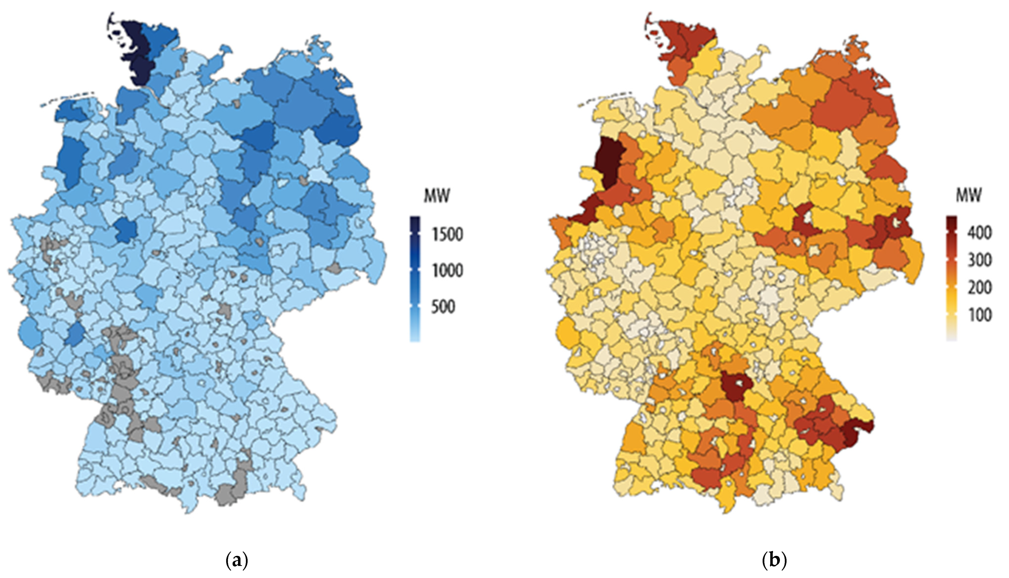
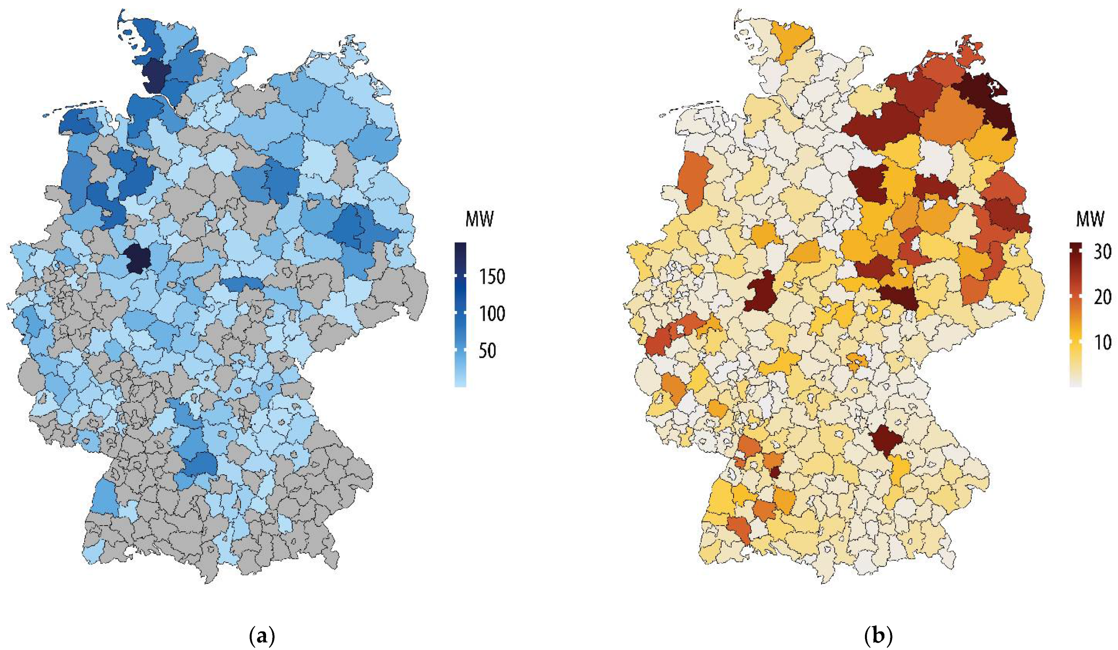
The initial information about onshore turbines in Germany with available data until the end of 2015 comes from the EE-monitor project [16], which can be freely downloaded from the UFZ data portal (www.ufz.de/drp (accessed on 5 March 2020)). As already known from various studies on renewable energies [5,6,17], turbine datasets for countries or widespread regions are hardly complete and often erroneous because of the high number of wind turbines with specific technical parameters. To mitigate this, appropriate machine learning methods are available to complete and improve the data of individual turbines with the knowledge about the residual plant ensemble. For the EE-monitor dataset, the random forests technique was used to close the existing gaps, applying as many predictor variables as possible [17]. To expand this turbine dataset to the whole of Germany and update it by the end of 2016, the missing plants of the German city states, as well as the plants erected in 2016, were inserted with the help of extra requested information from all federal states. Subsequently, all onshore turbines of the updated dataset were matched with the Core Energy Market Data Register (MaSTR) of the Federal Network Agency [18] by means of a spatial join. If the geographical location of the two plants were nearly equal in this data operation, i.e., having a horizontal distance of less than 75 m, the corresponding wind turbine data was completed with the available data from the MaSTR. Through this spatial join, the date of (de-)commissioning, the actual hub height (instead of the value predicted by random forests), and the turbine type could be often included in the plant dataset. Hence, the exact date of commissioning can be applied in many cases instead of the less accurate commissioning year, which allows the wind power model to account for plant changes during the investigated year. After filtering this compiled dataset for the year 2016, it comprises nearly 26 thousand onshore turbines corresponding to a capacity of 43.6 GW, depicted in Figure 1a as disaggregated spatial sums at NUTS-3 level. The total capacity reaches almost the officially installed capacity of 45.3 GW, according to the AGEE-Stat report [2], of all onshore wind turbines in Germany for 2016. A difference of less than 4% from this official value shows that most onshore turbines are contained in the final dataset.
The plant dataset of the photovoltaic systems comes from freely accessible data of the four Transmission System Operators (TSO) in Germany. After merging and filtering the raw data provided by the TSO on their information portal (www.netztransparenz.de (accessed on 30 July 2020)) [19], the final dataset contains more than 1.61 million photovoltaic systems for the year 2016. This compiled dataset, which was also compared with official figures [2,18], includes all roof-top and ground-mounted systems that obtain guaranteed feed-in tariff rates under the EEG. The installed capacity of the plant dataset has a total value of 40.4 GW, which almost agrees with the official sum of 40.7 GW in Germany for 2016 [2]. The corresponding installed capacity at NUTS-3 level is shown in Figure 1b.
2.2. Applied Weather Product
Verified weather products are a prerequisite for realistic modeling of the electricity production from variable renewables, and the spatiotemporal resolution of such data is crucial to the accuracy of the simulated time series. For Germany, weather products with various spatial and temporal resolutions are publicly available on the internet platforms of diverse meteorological services around the world. In recent years, reanalysis weather data have become a frequently used source for power generation simulations of variable renewables, especially for wind energy studies [6,7,8]. This kind of weather product is created using forecast models, re-running these numerical models for a given period in the past, and making final corrections with the help of measured data. Global reanalysis products, e.g., MERRA [20], MERRA-2 [21], and the more recent ERA5 data [22], generally provide a low horizontal resolution and, thus, do not match the level of geographical detail required for this work. Regional reanalysis products have usually higher spatial resolutions, e.g., the COSMO-REA6 data covering the entire German region with a horizontal resolution of approximately 6 km [23,24], which would already provide highly resolved results with the presented simulation models.
The numerical simulations performed for this publication go one step further and employ satellite-based weather data from the Satellite Application Facility on Climate Monitoring (CMSAF) collaboration [25] using the provided features of the Photovoltaic Geographical Information System (PVGIS) [26]. The CMSAF weather product via the web interface of PVGIS provides a spatial resolution of approximately 2.5 km and a temporal resolution of an hour for Germany. Moreover, the determination of solar irradiance on the ground from satellite images is calculated using complex algorithms, which do not only consider the highly resolved satellite data but also use atmospheric information on ozone, aerosols, and water vapor. Although these algorithms usually work very well they can also fail under certain conditions, e.g., snowy landscapes which can be misinterpreted as clouds. Thus, solar irradiances determined from satellite images should be verified by measurements on the ground in order to quantify the uncertainty of the radiation data. For the region of Germany, the accuracy of the CMSAF data is near the confidence level of measurements from terrestrial stations and is far better than the target accuracy of 10 W/m2 [27].
The time series provided by PVGIS (version 5.1) in hourly resolution for a desired period and location includes the following data required for the simulations: date and time, photovoltaic output power, ground elevation, air temperature at 2 m, and the wind speed at 10 m above the ground. Although the wind speed is only available at this low altitude, which may affect the accuracy of the extrapolated wind speed at turbine hub height, the weather data are provided accurately for each requested geographical location. This fact eliminates the need for further horizontal interpolations to the plant sites and, hence, the deviations caused by such interpolation routines, which may be higher than the loss of accuracy due to vertical wind speed extrapolations. In addition, PVGIS delivers the ground elevation for each onshore turbine location required for the estimation of the air pressure at hub height in the wind power model. Another advantage of retrieving the weather data via the PVGIS web interface is that the wind power and photovoltaic models can use the same weather product with, e.g., the same time base. This facilitates the mutual combinability and comparability of the simulation results.
2.3. Calibration and Validation Data
For a reasonable calibration of the simulation models and subsequent validation of the obtained results, additional data are necessary. For calibrating the wind power model, in particular, the power curves of the applied onshore turbines with their specific cut-in, rated, and cut-out speeds are required. These curves, which are usually provided as a table of values, describe the correlation between the wind speed at hub height and the output power of wind turbines achieved at a standardized air density of 1.225 kg/m3. Such power curves can be looked up in the datasheets of the turbine manufacturer or on the internet, e.g., at the wind energy platform (www.thewindpower.net (accessed on 25 June 2020)) [28].
The blue line in Figure 2a displays the plotted power curve of a typical onshore turbine including its specific parameters. The black points on this power curve show the discrete values from the datasheet of the manufacturer [29]. Figure 2b outlines the development process with all involved data from calibration to validation of the simulation models. In this flowchart, the input and output data are depicted as grey boxes and the arrows show the data flow.
For power losses of onshore turbines that are not covered by numerical calculations using the power curve, a corresponding reduction of the output power must be added in the simulation model. These additional turbine losses are mainly due to the following reasons:
- Power reduction because of mutual shading of adjacent turbines (wake effect).
- Loss of power due to ice or dirt on the rotor blades of the wind turbines.
- Feed-in interruptions because of energy surpluses in the power grids.
- Switch-offs due to turbine overhauls or bat and bird protection.
Since this information is not available for each individual wind turbine, such losses are considered as an overall reduction value of 16% in the wind power model. This value, which is usually between 5 and 30% for onshore turbines according to [30], has been shown in previous simulations to be a realistic average value for the investigated turbine ensemble.
Reasonable calibration data are also needed for the photovoltaic model. Since the technical parameters for each individual photovoltaic system are not fully known to the public, especially for the many existing small roof-top systems, realistic average values must be used in the simulation model as well. For example, the technology of the photovoltaic modules and the amount of the system loss have to be known for the simulations. This system loss describes all losses of a photovoltaic system that results in the electricity fed into the power grid being lower than that actually generated by the solar panels. There are various reasons for this loss, e.g., electrical losses in cables and power inverters of the plants or optical losses due to snow and dirt on the module surfaces. For the system loss, an overall value of 14% is recommended by PVGIS [26], which is applied to the entire ensemble of photovoltaic systems. The used solar cell technology is also not known for each individual plant. Up to now, crystalline silicon is the world’s most widely deployed semiconductor for photovoltaic modules [31]. Hence, crystalline silicon is chosen as semiconductor material for the simulations. Moreover, the azimuth and inclination angles of the photovoltaic modules are also required. The azimuth angle is set to zero for all photovoltaic systems, which means a fixed orientation of the solar panels in the southern direction. A fixed value of 20° is adopted for the inclination angle, since ground-mounted systems are typically erected with tilt angles in this range to reduce mutual shading of the photovoltaic modules, especially in winter when the maximum elevation angle of the sun reaches only low values [32]. Additionally, previous simulations have shown that 20° is also a reasonable average value for the existing roof-top systems.
In general, the results obtained with simulation models should be checked against measurements on real systems to verify the model algorithms and evaluate their accuracy. The used wind power and photovoltaic models have been validated with measurements of technically known single plants in [14,15]. However, the simulations presented in this study consider large ensembles of onshore turbines and photovoltaic systems. Thus, the simulation results showing the power generation from variable renewable energies have to be verified with measured feed-in data. Due to the lack of publicly available feed-in data of variable renewables with high spatial resolutions, it is not possible to verify the simulation results on a highly resolved spatial scale. But, if the simulated time series are spatially aggregated over the entire German region, they can be validated with measured feed-in patterns for all of Germany, which are freely accessible via the web interface of SMARD (www.smard.de (accessed on 18 March 2020)) [33]. Using this interface, the total feed-in from onshore wind turbines and photovoltaic systems were downloaded for 2016. It should be noted for this period that there were no measurements by SMARD on three days, so the concerned zero values are not taken into account in the validation and suppressed in the diagrams.
3. Models
The following subsections describe the simulation models for the electricity production from variable renewables employing publicly available plant and weather data. From a mathematical point of view, the power generation from these renewable energies can be determined either with statistical models, e.g., Monte Carlo and auto-regressive methods, or with physical models [6,7,34,35]. Opposed to statistical models [36,37], the simulation results of physical models, such as the presented wind power and photovoltaic models, are predicated on high-resolution data from weather models or real measurements. Thus, one benefit of physical over statistical models is the ability to create electricity production data on a highly resolved spatiotemporal scale.
3.1. Wind Power Model
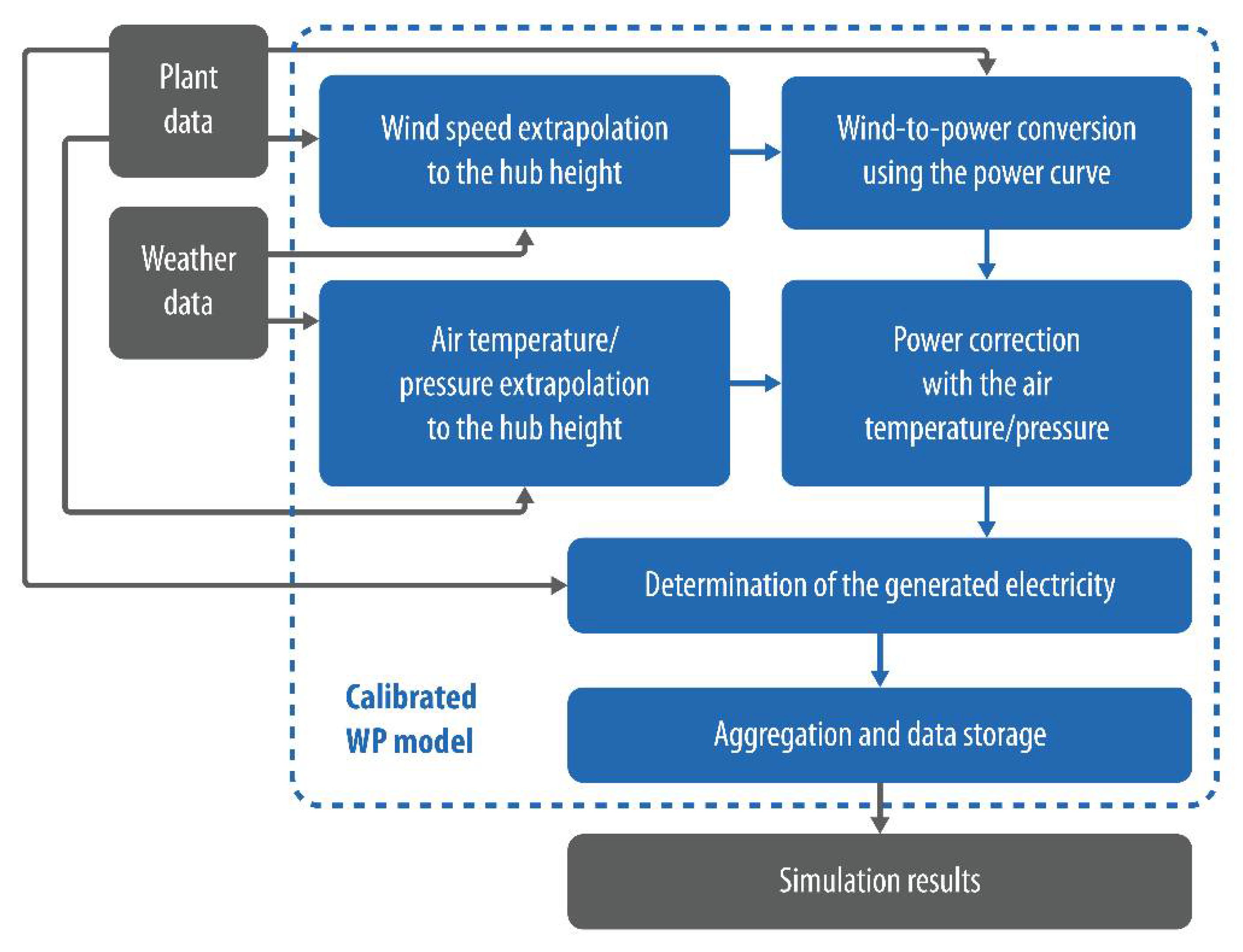
The main calculation steps and data flows of the wind power model are shown in Figure 3, where the plant and weather data are the input data for the calibrated simulation model. Herein, the calculation steps are depicted as blue boxes, and the other symbols have the same meaning as explained in the description of Figure 2b.
For this model, a new approach is used for the wind-to-power conversion, which employs a sixth-order polynomial approximation for the normalized power curve of a wind turbine. Once such an analytical representation is derived for a needed power curve, the output power can be easily calculated using the rated power of the onshore turbine along with the wind speed and the air temperature and pressure at its hub height. Since the type of a wind turbine is often not available, because of missing information from official sources [5], the turbines of the plant dataset are sorted into corresponding power classes with typical power curves. These classes with the assigned turbine type and range of rated power are listed in Table 2.
For example, for onshore turbines with a rated power of between 2500 and 3500 kW, the normalized power curve of a Vestas V112 with 3000 kW rated power is used for the numerical simulations. However, the geographical location, the date of (de-)commissioning, the rated power, and the hub height are taken into account individually for each wind turbine. In the subsequent calculation step, the achieved electricity production also considering additional losses and the date of commissioning is determined for each wind turbine. In the end, the simulated time series of the investigated turbine ensemble are converted into local time, aggregated in time, and saved as comma-separated values (CSV) for further data processing and use. A more detailed description of the wind power model with all the underlying physical laws, e.g., employing Hellmann’s law for the extrapolation of the wind speed to the hub height, and its properties can be found in [14].
3.2. Photovoltaic Model
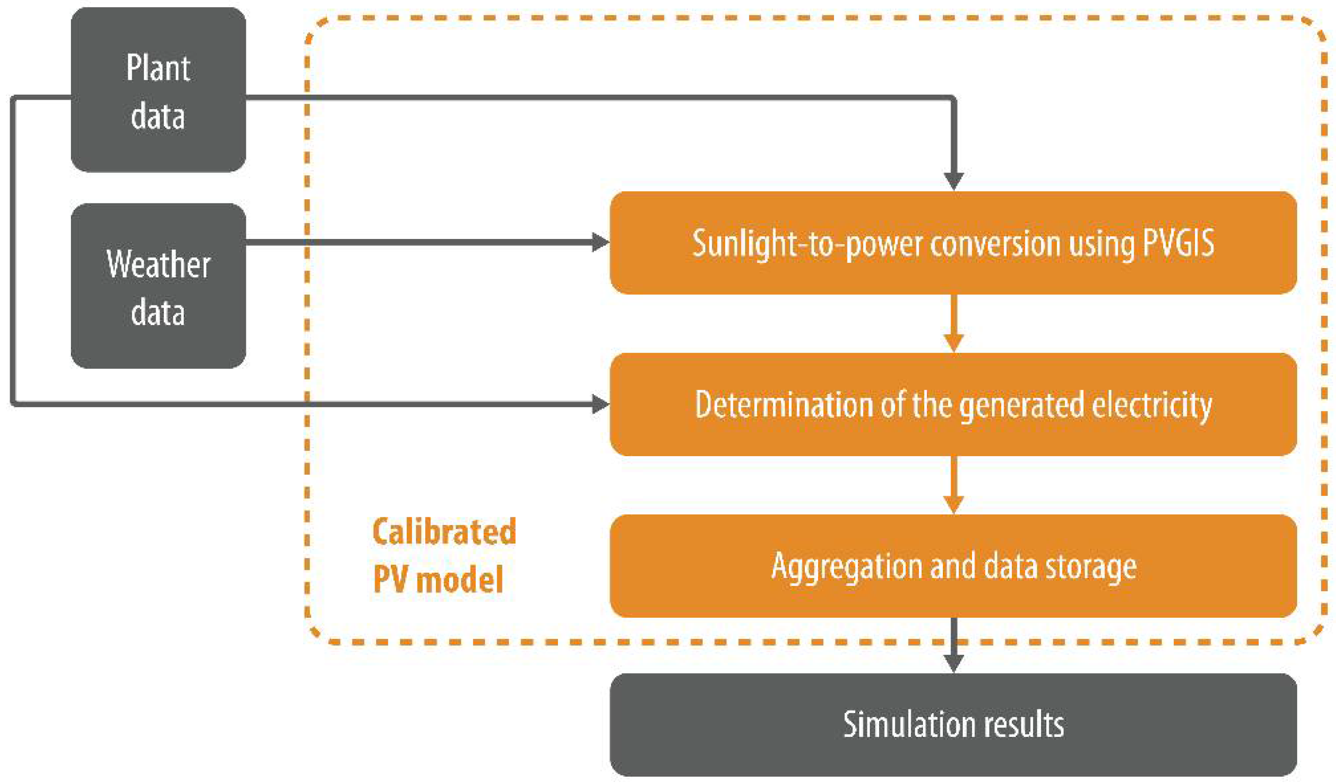
Figure 4 outlines the main calculation steps and data flows of the photovoltaic model. The calculation steps are drawn as orange boxes and the other symbols in the flowchart have the same meaning as already described in Figure 2b. As with the wind power model, the plant and weather data are required as input data for the calibrated simulation model.
This photovoltaic model can be structured into three successive calculation steps, as shown in Figure 4, which are carried out for the photovoltaic systems of the plant dataset. Firstly, the determination of the output power from the solar panels with the help of the sunlight-to-power algorithms of PVGIS [26]. Secondly, the calculation of the generated electricity considering the date of (de-)commissioning for each photovoltaic system. Thirdly and finally, the resulting time series of the entire ensemble are transformed into local time, temporally and spatially aggregated, and stored in CSV format for subsequent processing and use. A detailed explanation of the photovoltaic model and its characteristics can be found in [15].
4. Results
In this section, the simulation results obtained with the previously described input data and physical models are presented. The simulated time series are checked against measured feed-in data to validate the performed simulations and to discuss reasons for the existing deviations. After this, meaningful key figures for an energy transition atlas are derived and the achieved results are shown as high-resolution maps at NUTS-3 level. In this context, also the electricity consumption data of Germany for 2016 are scaled down to county level and related to the corresponding simulation results.
4.1. Wind Power Generation
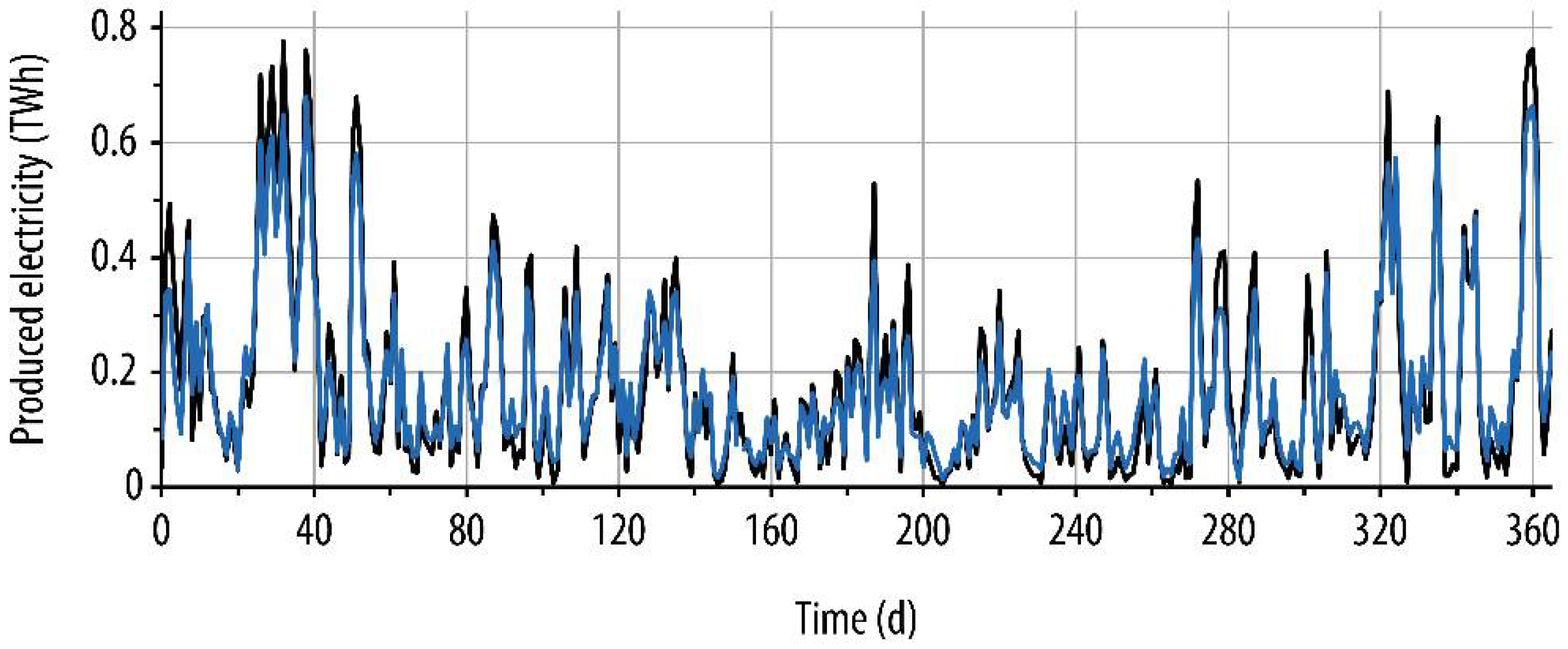
The wind power model is used to simulate the electricity production from onshore wind turbines in Germany for the year 2016. After model validation with measured wind speed and feed-in data of a technically known single turbine [14], the simulations were performed for an ensemble of nearly 26 thousand wind turbines. For these simulations, each turbine of the plant dataset was simulated individually and the weather data were retrieved via the PVGIS web interface for each turbine site, using its geographical position. As described in Section 2.3, for additional turbine losses an overall reduction value of 16% was applied to the entire plant ensemble. After carrying out the numerical simulations for all onshore turbines, the hourly resolved time series of the power generation were aggregated into one time series to check the simulation results against measured feed-in data for the whole of Germany. For better comparability and visual representation, the simulated and measured time series depicted in Figure 5 were transformed from hourly to daily resolutions.
In this diagram, it is easy to see that the simulated power generation matches the measured pattern well over the entire period. In addition, it is also visible in Figure 5 that most of the electricity is generated during the winter months. The existing deviations are primarily due to the following causes:
- Deviations caused by the wind speed extrapolation from 10 m to the hub height.
- The uncertainties of the weather data and the fact of hourly averaged values.
- Weather-related variations in air pressure are not considered in the model.
- The assignment of turbines to power classes with typical power curves.
The corresponding statistical measures for the daily values of both time series, as shown in Figure 5, are listed in the overview table of Section 4.3 for better comparability of all simulation results.
4.2. Photovoltaic Power Generation
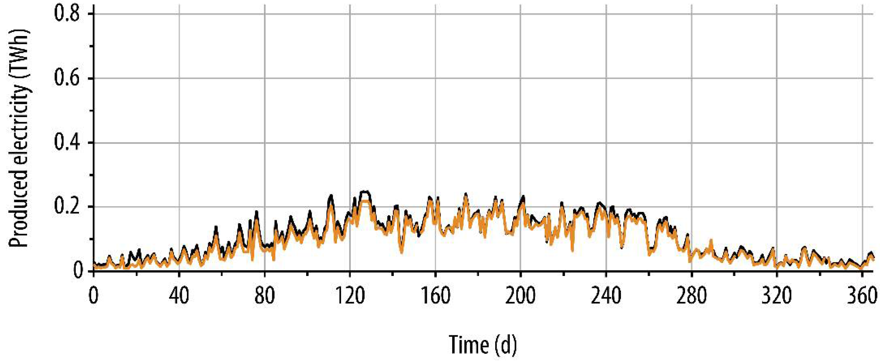
This section uses the photovoltaic model to simulate the electricity production from photovoltaic systems in Germany for the year 2016. After model validation with measured feed-in data of a technically known roof-top system [15], the simulations were carried out for the investigated ensemble. Due to the large number of more than 1.61 million single plants, the photovoltaic systems were sorted into their municipal areas and the center coordinates of these areas were used for the numerical simulations to limit the runtime. However, the date of (de-)commissioning and the peak power were considered individually for each photovoltaic system. Since no further information about these photovoltaic systems was publicly available, realistic average values (as given in Section 2.3) have to be used for a reasonable calibration of the photovoltaic model. After performing the simulations with the described calibration data, the hourly resolved time series were aggregated into one time series in order to check the simulation results against the measured feed-in from all photovoltaic systems in Germany. The simulated and measured power generation data are shown in Figure 6 with a daily resolution.
The simulated electricity production, as displayed in Figure 6, agrees well over the annual period with the measured pattern. Furthermore, it can be also deduced that most of the electricity is generated during the summer months. The resulting deviations have mainly the following reasons:
- The use of average values due to the lack of specific data for photovoltaic systems.
- The uncertainties of the weather data and the fact of hourly averaged values.
- Decrease of the power generation because of snow on the modules.
- Feed-in reductions due to energy surpluses or maintenance work.
The corresponding statistical measures for the daily values of the simulated and measured time series (Figure 6) are also given in the overview table of the next subsection.
4.3. Common Power Generation
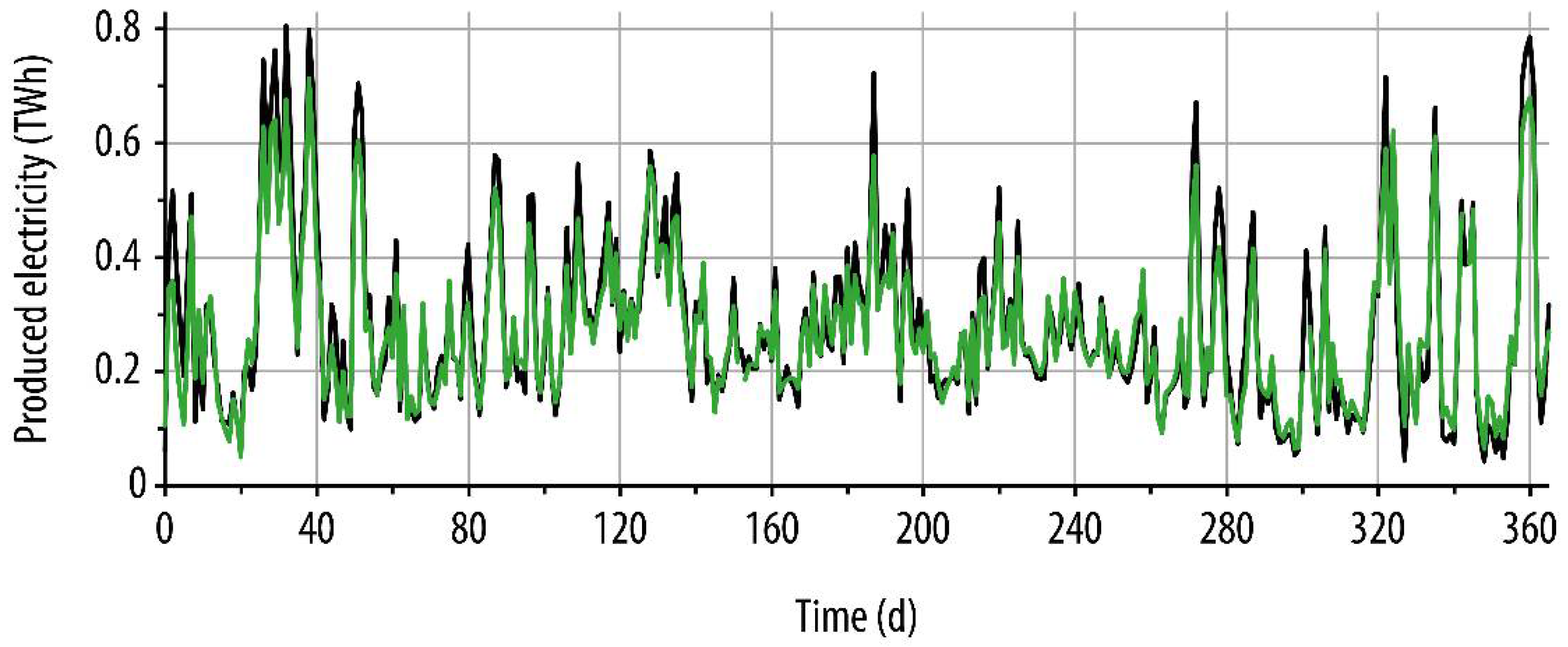
For a joint consideration of the presented variable renewables, which is very helpful for investigations on the energy transition in Germany, Figure 7 shows the sum of the daily electricity production from onshore turbines and photovoltaic systems.
In Figure 7 can be clearly seen that the common electricity production from these renewable energies also reproduces the measured feed-in pattern very well. With a Root-Mean-Square Error (RMSE) of 46.5 GWh determined for the daily values, as a statistical measure for the existing deviations, the joint simulation results show a high agreement with the measurements as well. In relation to the total electricity production of 97.9 TWh, generated by all onshore turbines and photovoltaic systems in Germany for 2016 [33], the RMSE reaches a value of 0.05%. As a further statistical evaluation of the simulation results, a Pearson correlation between the first differences for the daily values of both time series was applied according to Equation (1):
In this expression, RXY is the correlation coefficient (denoted as R-value in Table 3), Xi and Yi stand for the first differences of the simulated and measured time series of length n, and Xm and Ym are the corresponding mean values. This Pearson correlation shows a strong positive linear relationship with a correlation coefficient of 0.96, indicating that the trends of both time series vary in the same magnitude and direction. Table 3 gives an overview of the most important values and statistical measures for the individual and joint simulation results.
The numbers in this table also indicate that the calculated statistical measures of the joint simulation results correspond well with the individual simulations of the wind power and photovoltaic models. Table 3 additionally shows that onshore wind turbines have generated almost twice as much electricity as photovoltaic systems in Germany for 2016, although the installed wind turbine capacity was only 11% higher.
4.4. Energy Transition Atlas
Regional and local progress in transforming the power sector towards higher shares of variable renewables can be confidently tracked using spatiotemporal distributions of installed capacity and power generation. Thus, the plant datasets and simulation models presented in this work can enable closer monitoring of the energy transition in Germany. As a first example for such an energy transition atlas, Figure 8 displays the intra-annual capacity increase of onshore turbines and photovoltaic systems at NUTS-3 level for the year 2016.
Based on the numerical simulations performed for this paper, Figure 9 shows the monthly electricity production from variable renewables, i.e., onshore wind turbines and photovoltaic systems, at NUTS-3 level.
Moreover, understanding the impact of existing variable renewables on the power supply at a highly resolved spatial and temporal scale can be very helpful in identifying optimal pathways for a sustainable transition to de-carbonized power generation. For this, the simulation results presented in Figure 9 are related to the installed capacity data of variable renewable power plants (as depicted in Figure 1) to investigate their efficiency depending on the considered period and area. Similar to the definitions in [14,15], the spatiotemporal capacity factor CFst of variable renewables can be calculated by Equation (2):
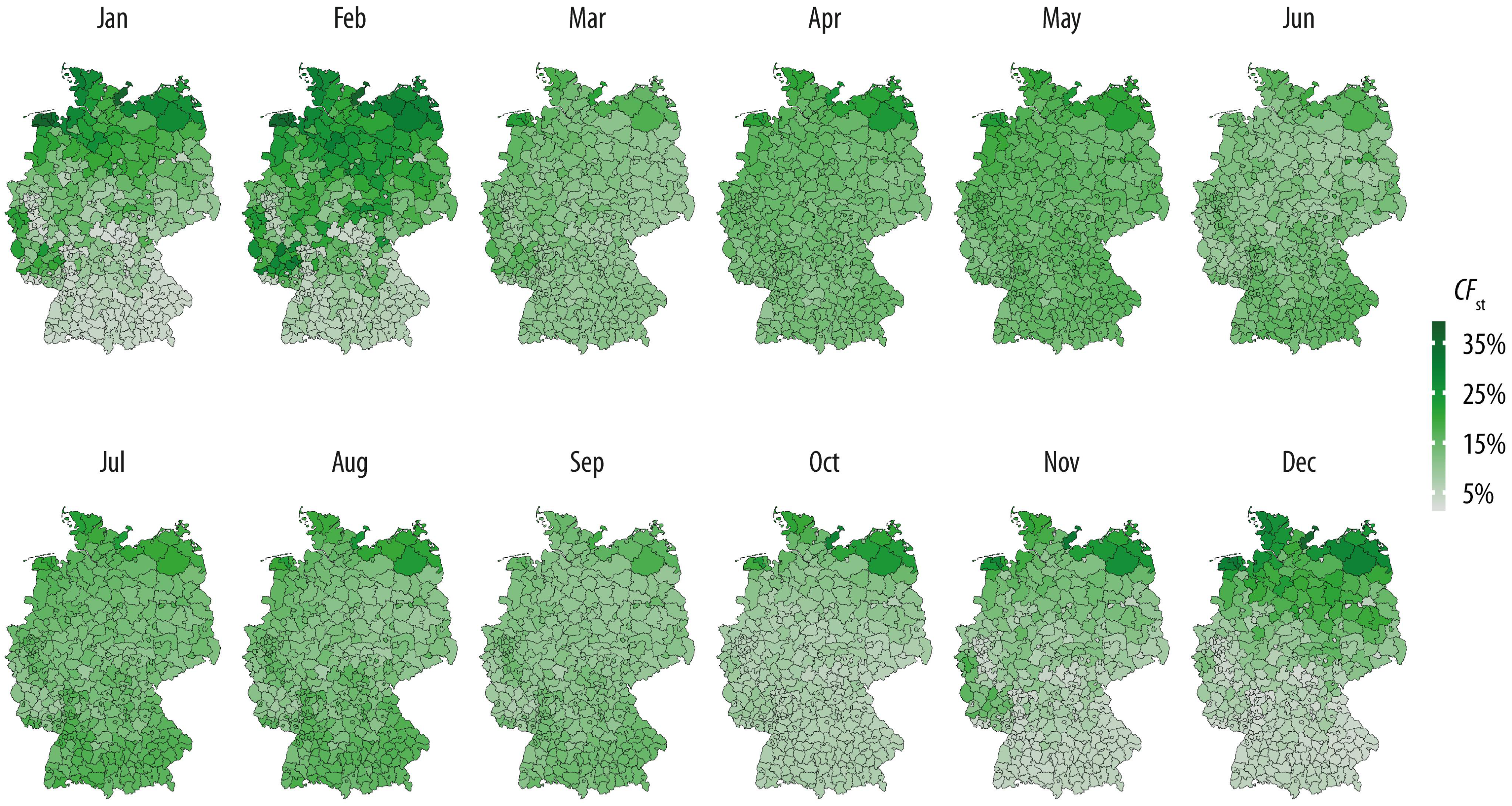
In this relationship, T stands for the specified period of time, Cvr is the sum of the onshore turbine and photovoltaic system capacity installed in the considered area, and Evr stands for the produced electricity from these renewable energies in this period and area. The following figure (Figure 10) shows the monthly capacity factors at NUTS-3 level in Germany for the year 2016.
From Figure 10, it can be derived that the capacity factors of variable renewables in the coastal regions of Germany were significantly higher from October till February than in the rest of 2016. This is mainly caused by the high wind power generation during the winter months. For this period, the electricity production from photovoltaic systems plays a minor role, which also leads to very low capacity factors in South Germany. In January and February, the spatiotemporal capacity factors rise to the highest values with an annual peak of 39% in the county of Emden. It is noteworthy as well that the northern areas of Germany, especially the coastal regions, have the highest capacity factors over the entire year due to the installed high wind turbine capacity. From November till February, the lowest capacity factors can be mainly found for 2016 in the southern parts of Germany and in the Rhine-Ruhr metropolitan region with values well below 10%.
In order to provide further insights into the energy transition in Germany, also the coverage rate of the power generation from variable renewables on the total electricity consumption is calculated on a highly resolved scale. For this, the disaggregated data from the numerical simulations are set in relation with the electricity consumption according to Equation (3):
In this expression, CRst describes the spatiotemporal coverage rate, Evr has the same meaning as for Equation (2), and Utot is the total electricity consumption in the considered period and area. In this context, a coverage rate of 100% means that the power generation from variable renewables fully offsets the electricity consumption. The total consumption is defined by the sum of electricity consumptions from the following four main sectors, household Uhh, trade and commerce Utc, industry Uin, and transport Utr, as given in Equation (4):
Since no pooled data on the electricity consumption at NUTS-3 level exist for the whole of Germany, publicly available data of the federal states are extrapolated to their counties using a top-down approach based on socioeconomic characteristics. The power consumption of households can be scaled down by the number of inhabitants and regional figures on real income, household, and apartment size [38,39,40,41,42,43]. The determination of the electricity consumption in the trade and commerce sector is based on the ratio of power consumption, population, gross domestic product, and real income [44]. The basic aspect of this consideration is that with a higher gross domestic product and a higher real income per capita, more services are provided and consumed, which leads to higher electricity consumption in this sector. The power consumption of industry is calculated on the basis of people which are employed in different industrial sectors. The calculation is based on the assumption that the production and processes in these sectors require approximately the same number of employees to be competitive, resulting in comparable electricity demand. The estimation for the transport sector refers only to electricity consumption in rail transport and is based on the relationship between power consumption, population, mobility behavior (expressed as distance traveled by public transport), and line supply. The data on electricity consumptions are from [45] and the figures on real income, household and apartment size, gross domestic product, employment, mobility behavior, and line supply are taken from [46,47].
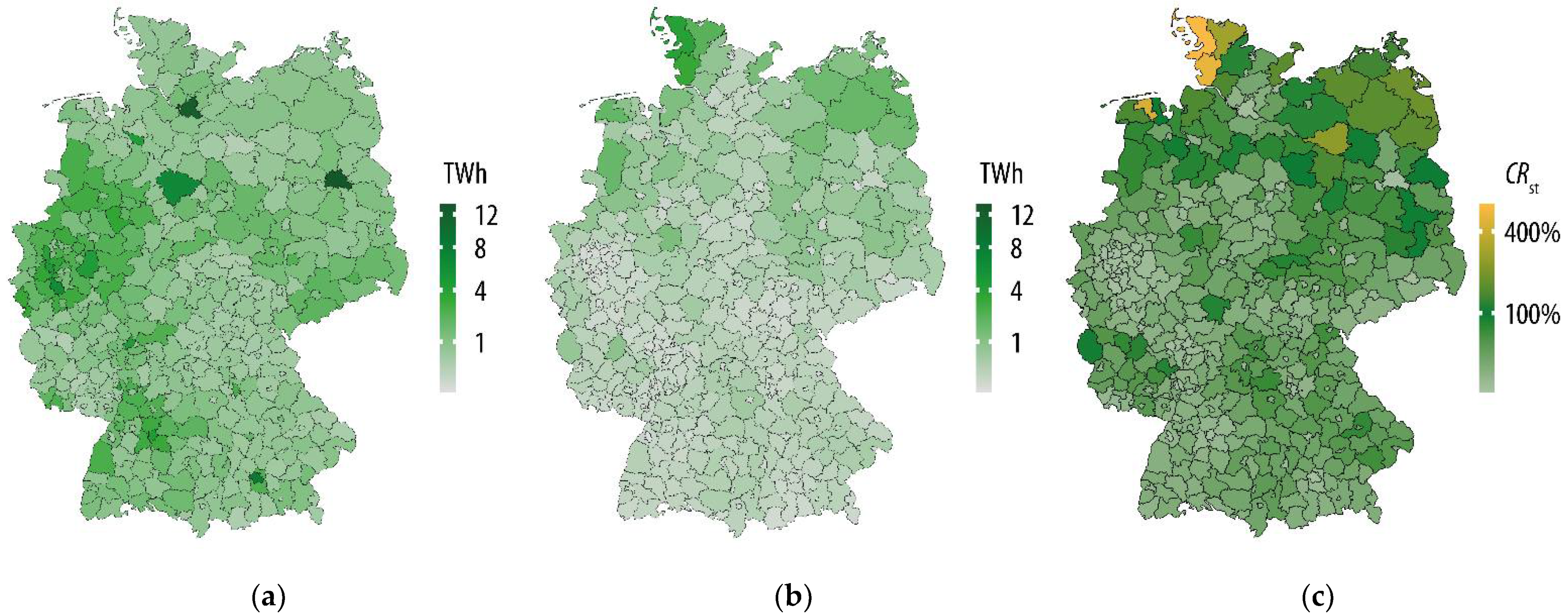
Using the information presented in Figure 11a,b for the investigated year, 2016, the coverage rate of the electricity production from variable renewables on the total electricity consumption can be determined according to Equation (3), which is depicted in Figure 11c at NUTS-3 level.
It can be easily seen in Figure 11c that the total electricity consumption, especially in urban areas with a high population density, like the metropolitan region of Rhine-Ruhr, is not sufficiently covered by variable renewables, i.e., the corresponding coverage rates are well below 10%. Furthermore, the three largest German cities, Berlin, Hamburg, and Munich, cover only a small share of their power consumption with self-generated variable renewable energies (with coverage rates of less than 5%), although there is potentially enough roof space for photovoltaic systems available. Due to the relatively high share of variable renewables in the northern and north-eastern parts of Germany combined with a low population density, coverage rates of about 100% are achieved for 2016, especially in some coastal regions with peak values above 400%.
5. Conclusions
One objective of this work was to create a highly resolved power generation time series of variable renewable energies in Germany for an annual period using publicly available plant and weather data. Herein, the focus was set on a joint consideration of the wind power and photovoltaic models and on a joint presentation of the simulation results. The year 2016 was chosen since the thoroughly compiled and verified plant datasets were only available until the end of 2016 at the time of writing. Nevertheless, the simulation models are applicable to other years and countries, if the required information about the renewable power plants is available. In addition, the presented models can be used with other weather products in PVGIS [26], which offer different resolutions and cover many countries of the world. For the numerical simulations performed in this study, an ensemble of nearly 1.64 million variable renewable power plants was taken into account. It could be shown that sufficiently precise simulation results can be achieved for onshore turbines and photovoltaic systems, i.e., the calculated power generation closely follows the measured feed-in pattern for all of Germany over the entire year. To the best of our knowledge, such highly resolved spatiotemporal electricity data of variable renewables using the same weather product for the wind power and photovoltaic models have never been shown before. Moreover, it is intended to make these simulation results also available on the data portal of the UFZ.
As a further objective of this paper, meaningful key figures for an energy transition atlas have been derived and the obtained results are presented as high-resolution maps at NUTS-3 level. In addition, this study has also combined highly resolved power generation time series from our simulation models with spatially downscaled electricity consumption data to gain further insights into the energy transition in Germany. Such data can be advantageous to investigate the multiple impacts of increasing variable renewables on local power systems or to find appropriate policy instruments to better meet the needs of different German regions. Many other applications, such as site assessment studies for wind farms [48] and photovoltaic systems [49,50], can also benefit from the presented results.
Author Contributions
Conceptualization, Reinhold Lehneis; Methodology, Reinhold Lehneis and David Manske; Software, Reinhold Lehneis and David Manske; Validation, Reinhold Lehneis; Formal Analysis, Reinhold Lehneis and David Manske; Investigation, Reinhold Lehneis; Resources, David Manske and Reinhold Lehneis; Data Curation, David Manske, Reinhold Lehneis and Björn Schinkel; Writing—Original Draft Preparation, Reinhold Lehneis; Writing—Review and Editing, Reinhold Lehneis, David Manske, Björn Schinkel and Daniela Thrän; Visualization, David Manske, Björn Schinkel and Reinhold Lehneis; Supervision, Reinhold Lehneis and Daniela Thrän; Project Administration, Daniela Thrän. All authors have read and agreed to the published version of the manuscript.
Funding
This research received general funding from the Helmholtz Association of German Research Centres.
Informed Consent Statement
Not applicable.
Conflicts of Interest
The authors declare no conflict of interest.
References
- GWEC. Global Wind Report 2021; Global Wind Energy Council: Brussels, Belgium, 2021. [Google Scholar]
- BMWi Time Series for the Development of Renewable Energy Sources in Germany Based on Statistical Data from the Working Group on Renewable Energy-Statistics (AGEE-Stat). Available online: https://www.erneuerbare-energien.de (accessed on 5 May 2021).
- IRENA. Renewable Power Generation Costs in 2019; International Renewable Energy Agency (IRENA): Abu Dhabi, United Arab Emirates, 2020. [Google Scholar]
- Rauner, S.; Eichhorn, M.; Thrän, D. The Spatial Dimension of the Power System: Investigating Hot Spots of Smart Renewable Power Provision. Appl. Energy 2016, 184, 1038–1050. [Google Scholar] [CrossRef]
- Eichhorn, M.; Scheftelowitz, M.; Reichmuth, M.; Lorenz, C.; Louca, K.; Schiffler, A.; Keuneke, R.; Bauschmann, M.; Ponitka, J.; Manske, D.; et al. Spatial Distribution of Wind Turbines, Photovoltaic Field Systems, Bioenergy, and River Hydro Power Plants in Germany. Data 2019, 4, 29. [Google Scholar] [CrossRef] [Green Version]
- Olauson, J.; Bergkvist, M. Modelling the Swedish Wind Power Production Using MERRA Reanalysis Data. Renew. Energy 2015, 76, 717–725. [Google Scholar] [CrossRef]
- Olauson, J. ERA5: The New Champion of Wind Power Modelling? Renew. Energy 2018, 126, 322–331. [Google Scholar] [CrossRef] [Green Version]
- Gruber, K.; Regner, P.; Wehrle, S.; Zeyringer, M.; Schmidt, J. Towards a Global Dynamic Wind Atlas: A Multi-Country Validation of Wind Power Simulation from MERRA-2 and ERA-5 Reanalyses Bias-Corrected with the Global Wind Atlas. arXiv 2020, arXiv:2012.05648. [Google Scholar]
- Olauson, J.; Bergkvist, M. Correlation between Wind Power Generation in the European Countries. Energy 2016, 114, 663–670. [Google Scholar] [CrossRef]
- Ramirez Camargo, L.; Stoeglehner, G. Spatiotemporal Modelling for Integrated Spatial and Energy Planning. Energy Sustain. Soc. 2018, 8, 32. [Google Scholar] [CrossRef]
- Hawkins, S.; Eager, D.; Harrison, G.P. Characterising the Reliability of Production from Future British Offshore Wind Fleets. In Proceedings of the IET Conference on Renewable Power Generation, Hertfordshire, UK, 6–8 September 2011; p. 212. [Google Scholar] [CrossRef] [Green Version]
- Kiss, P.; Varga, L.; Jánosi, I.M. Comparison of Wind Power Estimates from the ECMWF Reanalyses with Direct Turbine Measurements. J. Renew. Sustain. Energy 2009, 1, 033105. [Google Scholar] [CrossRef] [Green Version]
- Lehneis, R.; Manske, D.; Schinkel, B.; Thrän, D. Modeling of the Power Generation from Wind Turbines with High Spatial and Temporal Resolution. EGU Gen. Assem. Conf. Abstr. 2020. [Google Scholar] [CrossRef]
- Lehneis, R.; Manske, D.; Thrän, D. Modeling of the German Wind Power Production with High Spatiotemporal Resolution. ISPRS Int. J. Geo-Inf. 2021, 10, 104. [Google Scholar] [CrossRef]
- Lehneis, R.; Manske, D.; Thrän, D. Generation of Spatiotemporally Resolved Power Production Data of PV Systems in Germany. ISPRS Int. J. Geo-Inf. 2020, 9, 621. [Google Scholar] [CrossRef]
- Thrän, D.; Bunzel, K.; Klenke, R.; Koblenz, B.; Lorenz, C.; Majer, S.; Manske, D.; Massmann, E.; Oehmichen, G.; Peters, W.; et al. Naturschutzfachliches Monitoring des Ausbaus der Erneuerbaren Energien im Strombereich und Entwicklung von Instrumenten zur Verminderung der Beeinträchtigung von Natur und Landschaft; Bundesamt für Naturschutz: Bonn, Germany, 2020. [Google Scholar]
- Becker, R.; Thrän, D. Completion of Wind Turbine Data Sets for Wind Integration Studies Applying Random Forests and K-Nearest Neighbors. Appl. Energy 2017, 208, 252–262. [Google Scholar] [CrossRef]
- Federal Network Agency Core Energy Market Data Register. Available online: https://www.bundesnetzagentur.de/EN (accessed on 30 July 2020).
- EEG-Anlagestammdaten. Available online: https://www.netztransparenz.de/ (accessed on 30 July 2020).
- Rienecker, M.M.; Suarez, M.J.; Gelaro, R.; Todling, R.; Bacmeister, J.; Liu, E.; Bosilovich, M.G.; Schubert, S.D.; Takacs, L.; Kim, G.-K.; et al. MERRA: NASA’s Modern-Era Retrospective Analysis for Research and Applications. J. Clim. 2011, 24, 3624–3648. [Google Scholar] [CrossRef]
- Gelaro, R.; McCarty, W.; Suárez, M.J.; Todling, R.; Molod, A.; Takacs, L.; Randles, C.A.; Darmenov, A.; Bosilovich, M.G.; Reichle, R.; et al. The Modern-Era Retrospective Analysis for Research and Applications, Version 2 (MERRA-2). J. Clim. 2017, 30, 5419–5454. [Google Scholar] [CrossRef] [PubMed]
- Hersbach, H.; Bell, B.; Berrisford, P.; Hirahara, S.; Horányi, A.; Muñoz-Sabater, J.; Nicolas, J.; Peubey, C.; Radu, R.; Schepers, D.; et al. The ERA5 Global Reanalysis. Q. J. R. Meteorol. Soc. 2020, 146, 1999–2049. [Google Scholar] [CrossRef]
- Bollmeyer, C.; Keller, J.D.; Ohlwein, C.; Wahl, S.; Crewell, S.; Friederichs, P.; Hense, A.; Keune, J.; Kneifel, S.; Pscheidt, I.; et al. Towards a High-Resolution Regional Reanalysis for the European CORDEX Domain. Q. J. R. Meteorol. Soc. 2015, 141, 1–15. [Google Scholar] [CrossRef]
- Frank, C.W.; Wahl, S.; Keller, J.D.; Pospichal, B.; Hense, A.; Crewell, S. Bias Correction of a Novel European Reanalysis Data Set for Solar Energy Applications. Sol. Energy 2018, 164, 12–24. [Google Scholar] [CrossRef]
- Satellite Application Facility on Climate Monitoring (CM SAF). Available online: https://www.cmsaf.eu/EN/Home/home_node.html (accessed on 18 March 2020).
- EU Science Hub-Photovoltaic Geographical Information System (PVGIS). Available online: https://ec.europa.eu/jrc/en/pvgis (accessed on 25 June 2020).
- Mueller, R.W.; Matsoukas, C.; Gratzki, A.; Behr, H.D.; Hollmann, R. The CM-SAF Operational Scheme for the Satellite Based Retrieval of Solar Surface Irradiance—A LUT Based Eigenvector Hybrid Approach. Remote Sens. Environ. 2009, 113, 1012–1024. [Google Scholar] [CrossRef]
- Pierrot, M. The Wind Power. Available online: https://www.thewindpower.net/ (accessed on 25 June 2020).
- Datasheet ENERCON E-40/5.40; ENERCON GmbH, Dreekamp 5: Aurich, Germany, 2003.
- Krebs, H.; Kuntzsch, J. Betriebserfahrungen Mit Windkraftanlagen Auf Komplexen Binnenlandstandorten. Erneuerbare Energy 2000, 12, 2000. [Google Scholar]
- Hosenuzzaman, M.; Rahim, N.A.; Selvaraj, J.; Hasanuzzaman, M.; Malek, A.B.M.A.; Nahar, A. Global Prospects, Progress, Policies, and Environmental Impact of Solar Photovoltaic Power Generation. Renew. Sustain. Energy Rev. 2015, 41, 284–297. [Google Scholar] [CrossRef]
- Krömke, F. Ertragsgutachten-PV Freiflächenanlage BEMA Halde Korbwerder, Sachsen-Anhalt, Deutschland. Available online: https://www.helionat.de/ (accessed on 31 August 2020).
- SMARD-Strommarktdaten. Available online: https://www.smard.de/home/ (accessed on 18 March 2020).
- Lu, L.; Yang, H.X. A Study on Simulations of the Power Output and Practical Models for Building Integrated Photovoltaic Systems. J. Sol. Energy Eng. 2004, 126, 929–935. [Google Scholar] [CrossRef]
- Brecl, K.; Topič, M. Photovoltaics (PV) System Energy Forecast on the Basis of the Local Weather Forecast: Problems, Uncertainties and Solutions. Energies 2018, 11, 1143. [Google Scholar] [CrossRef] [Green Version]
- Ekström, J.; Koivisto, M.; Mellin, I.; Millar, R.J.; Lehtonen, M. A Statistical Modeling Methodology for Long-Term Wind Generation and Power Ramp Simulations in New Generation Locations. Energies 2018, 11, 2442. [Google Scholar] [CrossRef] [Green Version]
- Benth, F.E.; Ibrahim, N.A. Stochastic Modeling of Photovoltaic Power Generation and Electricity Prices. J. Energy Mark. 2017, 10, 1–33. [Google Scholar] [CrossRef] [Green Version]
- Zhou, Q.; Bialek, J.W. Approximate Model of European Interconnected System as a Benchmark System to Study Effects of Cross-Border Trades. IEEE Trans. Power Syst. 2005, 20, 782–788. [Google Scholar] [CrossRef]
- Sonnberger, M.; Zwick, M.M. Der Energieverbrauch in Privathaushalten soziologisch betrachtet. Soziol. Nachhalt. 2016, 2, 1–28. [Google Scholar] [CrossRef]
- Huebner, G.; Shipworth, D.; Hamilton, I.; Chalabi, Z.; Oreszczyn, T. Understanding Electricity Consumption: A Comparative Contribution of Building Factors, Socio-Demographics, Appliances, Behaviours and Attitudes. Appl. Energy 2016, 177, 692–702. [Google Scholar] [CrossRef] [Green Version]
- Abrahamse, W.; Steg, L. Factors Related to Household Energy Use and Intention to Reduce It: The Role of Psychological and Socio-Demographic Variables. Hum. Ecol. Rev. 2011, 18, 30–40. [Google Scholar]
- Brohmann, B.; Heinzle, S.; Rennings, K.; Schleich, J.; Wüstenhagen, R. What’s Driving Sustainable Energy Consumption? A Survey of the Empirical Literature; Zentrum für Europäische Wirtschaftsforschung: Mannheim, Germany, 2009. [Google Scholar]
- Guerin, D.A.; Yust, B.L.; Coopet, J.G. Occupant Predictors of Household Energy Behavior and Consumption Change as Found in Energy Studies Since 1975. Fam. Consum. Sci. Res. J. 2000, 29, 48–80. [Google Scholar] [CrossRef]
- Soytas, U.; Sari, R. Energy Consumption and GDP: Causality Relationship in G-7 Countries and Emerging Markets. Energy Econ. 2003, 25, 33–37. [Google Scholar] [CrossRef]
- LAK Länderarbeitskreises Energiebilanzen. Available online: https://www.lak-energiebilanzen.de/ (accessed on 22 July 2020).
- Statistische Ämter Statistische Ämter des Bundes und der Länder. Available online: http://www.statistikportal.de/de (accessed on 27 July 2020).
- MiD. Mobilität in Deutschland; Bundesministerium für Verkehr und digitale Infrastruktur (BMVI): Berlin, Germany, 2020. [Google Scholar]
- Becker, R.; Thrän, D. Optimal Siting of Wind Farms in Wind Energy Dominated Power Systems. Energies 2018, 11, 978. [Google Scholar] [CrossRef] [Green Version]
- Choi, Y.; Suh, J.; Kim, S.-M. GIS-Based Solar Radiation Mapping, Site Evaluation, and Potential Assessment: A Review. Appl. Sci. 2019, 9, 1960. [Google Scholar] [CrossRef] [Green Version]
- Guaita-Pradas, I.; Marques-Perez, I.; Gallego, A.; Segura, B. Analyzing Territory for the Sustainable Development of Solar Photovoltaic Power Using GIS Databases. Environ. Monit Assess 2019, 191, 764. [Google Scholar] [CrossRef] [PubMed] [Green Version]
Figure 1.
Installed capacity of (a) onshore turbines and (b) photovoltaic systems shown as spatial sums at NUTS-3 level in Germany for the year 2016. In the grey areas of Figure 1a no wind turbines are installed.
Figure 1.
Installed capacity of (a) onshore turbines and (b) photovoltaic systems shown as spatial sums at NUTS-3 level in Germany for the year 2016. In the grey areas of Figure 1a no wind turbines are installed.

Figure 2.
(a) Plotted power curve (blue line) of an Enercon E-40 with 500 kW rated power as an example for a typical onshore turbine. (b) Flowchart of the development process with all involved data from calibration to validation of the simulation models.
Figure 2.
(a) Plotted power curve (blue line) of an Enercon E-40 with 500 kW rated power as an example for a typical onshore turbine. (b) Flowchart of the development process with all involved data from calibration to validation of the simulation models.
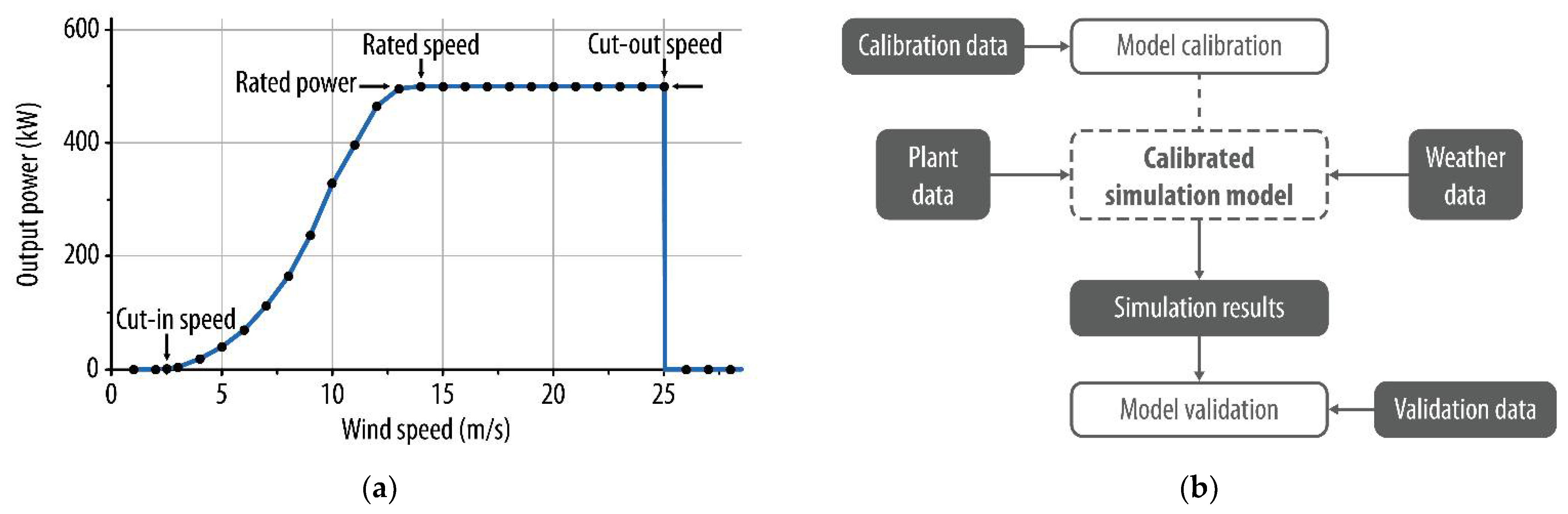
Figure 3.
Flowchart of the wind power (WP) model showing the calculation steps and data flows.

Figure 4.
Flowchart of the photovoltaic (PV) model showing the calculation steps and data flows.

Figure 5.
Simulated (black line) and measured (blue line) feed-in patterns of all onshore turbines in Germany for 2016.
Figure 5.
Simulated (black line) and measured (blue line) feed-in patterns of all onshore turbines in Germany for 2016.

Figure 6.
Simulated (black line) and measured (orange line) feed-in patterns of all photovoltaic systems in Germany for 2016.
Figure 6.
Simulated (black line) and measured (orange line) feed-in patterns of all photovoltaic systems in Germany for 2016.

Figure 7.
Simulated (black line) and measured (green line) feed-in patterns of variable renewables, i.e., onshore turbines and photovoltaic systems, in Germany for 2016.
Figure 7.
Simulated (black line) and measured (green line) feed-in patterns of variable renewables, i.e., onshore turbines and photovoltaic systems, in Germany for 2016.

Figure 8.
Intra-annual increase of installed (a) onshore turbine and (b) photovoltaic system capacity at NUTS-3 level in Germany for 2016. In the grey areas of Figure 8a no wind turbines have been added during this year.
Figure 8.
Intra-annual increase of installed (a) onshore turbine and (b) photovoltaic system capacity at NUTS-3 level in Germany for 2016. In the grey areas of Figure 8a no wind turbines have been added during this year.

Figure 9.
Monthly electricity production from variable renewables at NUTS-3 level in Germany for 2016.
Figure 9.
Monthly electricity production from variable renewables at NUTS-3 level in Germany for 2016.
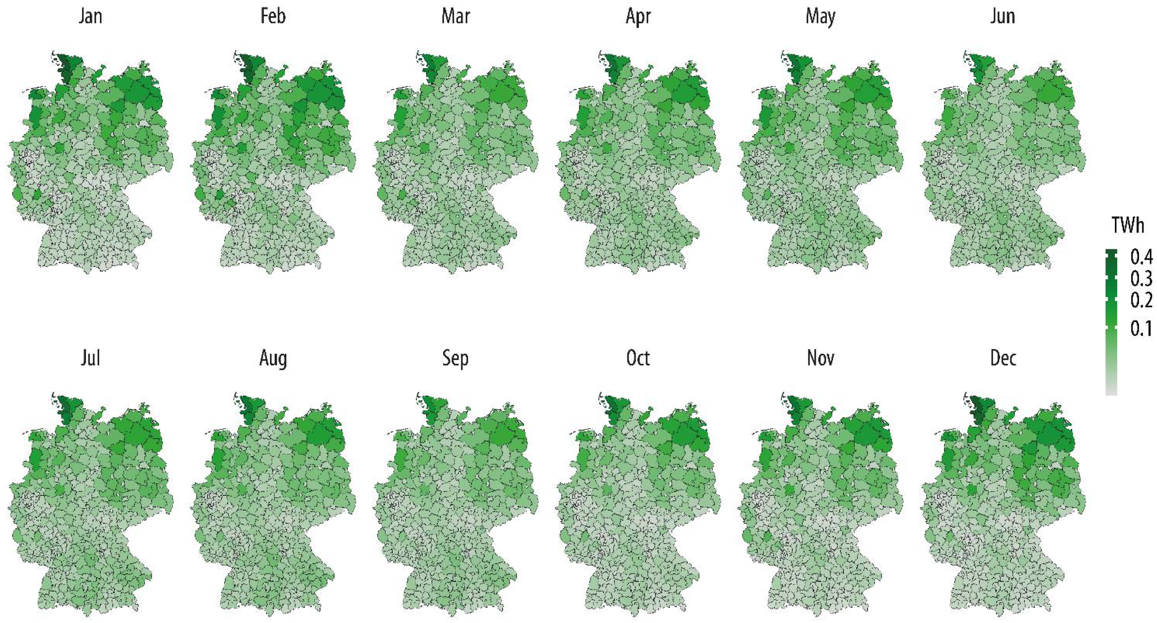
Figure 10.
Monthly capacity factors of variable renewables at NUTS-3 level in Germany for 2016.

Figure 11.
Spatially resolved values of the (a) total electricity consumption, (b) annual electricity production from variable renewable energies, and (c) coverage rate reached with variable renewables at NUTS-3 level in Germany for 2016.
Figure 11.
Spatially resolved values of the (a) total electricity consumption, (b) annual electricity production from variable renewable energies, and (c) coverage rate reached with variable renewables at NUTS-3 level in Germany for 2016.


Table 1.
Parameters of the plant datasets necessary for the wind power and photovoltaic models.
| Parameter | Wind Power Model | Photovoltaic Model |
|---|---|---|
| Latitude | required | optional |
| Longitude | required | optional |
| LAU-Id 1 | optional | required |
| Commission date | required | required |
| Decommission date | optional | optional |
| Rated power | required | required |
| Hub height | required | not applicable |
| Rotor diameter | not applicable | not applicable |
| Turbine type | optional | not applicable |
1 The LAU-Id is an eight-digit identifier for the unique determination of a local administrative unit (LAU).
Table 2.
The used power classes with the assigned turbine type and range of rated power (PR).
| Power Class (kW) | Turbine Type | Power Range (kW) |
|---|---|---|
| 100 | Fuhrländer FL100 | PR ≤ 150 |
| 200 | Enercon E-30 | 150 < PR ≤ 250 |
| 500 | Enercon E-40 | 250 < PR ≤ 750 |
| 1000 | Vestas V52 | 750 < PR ≤ 1500 |
| 2000 | Enercon E-82 | 1500 < PR ≤ 2500 |
| 3000 | Vestas V112 | 2500 < PR ≤ 3500 |
| 5000 | Enercon E-126 | PR > 3500 |
Table 3.
Installed capacity, feed-in, and statistical measures for the simulation results.
| Data | Onshore Turbines | Photovoltaics | Common Values |
|---|---|---|---|
| Installed capacity | 45.3 GW | 40.7 GW | 86.0 GW |
| Feed-in | 64.0 TWh | 33.9 TWh | 97.9 TWh |
| RMSE | 45.6 GWh | 13.9 GWh | 46.5 GWh |
| RMSE/Feed-in | 0.07% | 0.04% | 0.05% |
| R-value | 0.97 | 0.97 | 0.96 |
Publisher’s Note: MDPI stays neutral with regard to jurisdictional claims in published maps and institutional affiliations. |
© 2022 by the authors. Licensee MDPI, Basel, Switzerland. This article is an open access article distributed under the terms and conditions of the Creative Commons Attribution (CC BY) license (https://creativecommons.org/licenses/by/4.0/).
Share and Cite
MDPI and ACS Style
Lehneis, R.; Manske, D.; Schinkel, B.; Thrän, D. Spatiotemporal Modeling of the Electricity Production from Variable Renewable Energies in Germany. ISPRS Int. J. Geo-Inf. 2022, 11, 90. https://doi.org/10.3390/ijgi11020090
AMA Style
Lehneis R, Manske D, Schinkel B, Thrän D. Spatiotemporal Modeling of the Electricity Production from Variable Renewable Energies in Germany. ISPRS International Journal of Geo-Information. 2022; 11(2):90. https://doi.org/10.3390/ijgi11020090
Chicago/Turabian StyleLehneis, Reinhold, David Manske, Björn Schinkel, and Daniela Thrän. 2022. "Spatiotemporal Modeling of the Electricity Production from Variable Renewable Energies in Germany" ISPRS International Journal of Geo-Information 11, no. 2: 90. https://doi.org/10.3390/ijgi11020090
Note that from the first issue of 2016, this journal uses article numbers instead of page numbers. See further details here.