Modeling Urban Land Cover Growth Dynamics Using Multi‑Temporal Satellite Images: A Case Study of Dhaka, Bangladesh


Abstract
:
1. Introduction
1.1. Background of the Research
1.2. Existing Works
2. Materials
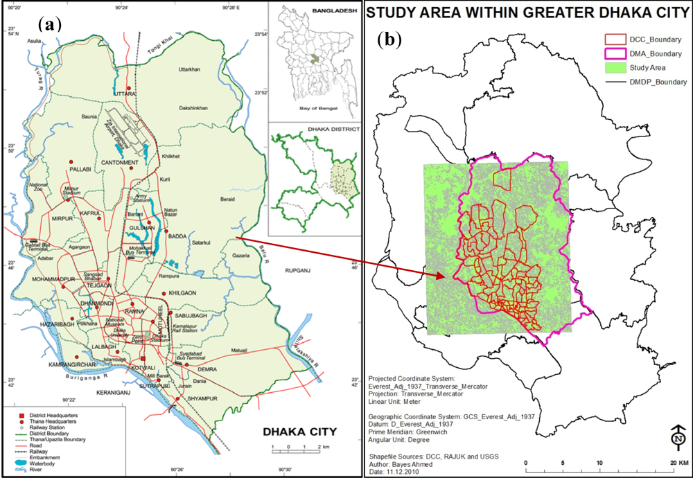
2.1. Study Area
2.2. Remote Sensing Data


| Land Cover Type | Description |
|---|---|
| Built-up Area | All residential, commercial and industrial areas, villages, settlements and transportation infrastructure. |
| Water Body | River, permanent open water, lakes, ponds, canals and reservoirs. |
| Vegetation | Trees, shrub lands and semi natural vegetation: deciduous, coniferous, and mixed forest, palms, orchard, herbs, climbers, gardens, inner-city recreational areas, parks and playgrounds, grassland and vegetable lands. |
| Low Land | Permanent and seasonal wetlands, low-lying areas, marshy land, rills and gully, swamps, mudflats, all cultivated areas including urban agriculture; crop fields and rice-paddies. |
| Fallow Land | Fallow land, earth and sand land in-fillings, construction sites, developed land, excavation sites, solid waste landfills, open space, bare and exposed soils. |
| Respective Year | Date Acquired (Day/Month/Year) | Sensor |
|---|---|---|
| 1989 | 13/02/1989 | Landsat 4–5 Thematic Mapper (TM) |
| 1999 | 24/11/1999 | Landsat 7 Enhanced Thematic Mapper Plus (ETM+) |
| 2009 | 26/10/2009 | Landsat 4–5 Thematic Mapper (TM) |
2.3. Base Map Preparation
2.3.1. Training Site Development
2.3.2. Signature Development
2.3.3. Classification
2.3.4. Generalization

2.4. Accuracy Assessment
2.4.1. User’s, Producer’s and Overall Accuracy
| Class Name | Reference Totals | Classified Totals | Number Correct | Producer’s Accuracy | User’s Accuracy |
|---|---|---|---|---|---|
| Built-up Area | 18 | 21 | 18 | 100.00% | 85.71% |
| Water Body | 46 | 38 | 35 | 76.09% | 92.11% |
| Vegetation | 66 | 61 | 54 | 81.82% | 88.52% |
| Low Land | 43 | 35 | 31 | 72.09% | 88.57% |
| Fallow Land | 77 | 95 | 75 | 97.40% | 78.95% |
| Totals | 250 | 250 | 213 |
| Class Name | Reference Totals | Classified Totals | Number Correct | Producer’s Accuracy | User’s Accuracy |
|---|---|---|---|---|---|
| Built-up Area | 62 | 72 | 60 | 96.77% | 83.33% |
| Water Body | 28 | 24 | 20 | 71.43% | 83.33% |
| Vegetation | 56 | 53 | 47 | 83.93% | 88.68% |
| Low Land | 33 | 30 | 29 | 87.88% | 96.67% |
| Fallow Land | 250 | 250 | 217 | 85.92% | 85.92% |
| Totals | 250 | 250 | 217 |
| Class Name | Reference Totals | Classified Totals | Number Correct | Producer’s Accuracy | User’s Accuracy |
|---|---|---|---|---|---|
| Built-up Area | 112 | 115 | 108 | 96.43% | 93.91% |
| Water Body | 22 | 19 | 17 | 77.27% | 89.47% |
| Vegetation | 43 | 45 | 41 | 95.35% | 91.11% |
| Low Land | 28 | 28 | 24 | 85.71% | 85.71% |
| Fallow Land | 45 | 43 | 39 | 86.67% | 90.70% |
| Totals | 250 | 250 | 229 |
2.4.2. Map Error vs. the Amount of Differences among the Maps
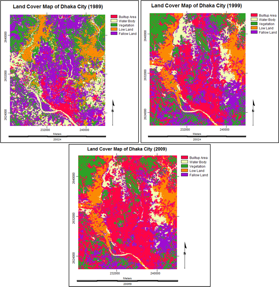
| Land Cover Type | 1989 | 1999 | Change in Area (%)(1989–1999) | ||
|---|---|---|---|---|---|
| Area (km2) | % | Area (km2) | % | ||
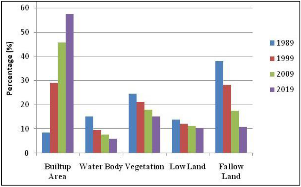
| Built-up Area | 37.6569 | 8.447 | 129.2292 | 28.991 | +20.544 |
| Water Body | 67.3218 | 15.102 | 42.5034 | 9.535 | −5.567 |
| Vegetation | 109.5714 | 24.581 | 94.3929 | 21.175 | −3.406 |
| Low Land | 62.0640 | 13.923 | 53.7264 | 12.052 | −1.871 |
| Fallow Land | 169.1559 | 37.947 | 125.9181 | 28.247 | −9.70 |
| Total | 445.770 | 100 | 445.770 | 100 | 0 |
| Land Cover Type | 1999 | 2009 | Change in Area (%)(1999–2009) | ||
|---|---|---|---|---|---|
| Area (km2) | % | Area (km2) | % | ||
| Built-up Area | 129.2292 | 28.991 | 204.4008 | 45.853 | +16.862 |
| Water Body | 42.5034 | 9.535 | 33.6645 | 7.552 | −1.983 |
| Vegetation | 94.3929 | 21.175 | 79.9578 | 17.937 | −3.238 |
| Low Land | 53.7264 | 12.052 | 49.9914 | 11.215 | −0.837 |
| Fallow Land | 125.9181 | 28.247 | 77.7555 | 17.443 | −10.804 |
| Total | 445.770 | 100 | 445.770 | 100 | 0 |
2.4.3. Limitations in Base Map Preparation and Accuracy Assessment
- The same spectral characteristics of some land cover types. For example, in case of 1989 base map, certain built-up areas were misclassified as fallow land. Again, in most cases it was really difficult to separate water bodies and low/cultivable lands categories. The reasons may be the seasonal variations of the satellite images for different years and the similar spectral properties of land covers in some cases. The images collected for 1999 (November) and 2009 (October) are from the same winter season. But the image of 1989 (February) is from another season, summer. This kind of variation creates problems while preparing base maps for analysis.
- Moreover, less image spectral resolution has directed to spectral mixing of different land cover types. This has caused spectral confusions among the cover types. It is also important to mention that the images of 1999 and 2009 represent winter season while the image of 1989 represents spring season. Therefore other seasonal images can be important evaluating the land cover change pattern of this kind of highly dynamic urban environment like Dhaka.
- Again the spatial resolution of the images is important. For this research purpose, Landsat satellite images have been chosen that are only commercially available but can be found in free public-domain. The main problem of working with Landsat images is low resolution. The spatial resolution of Landsat Image is 30 m. IKONOS, QuickBird or other satellite images with higher resolution can be better option.
- The next limitation regarding this research is the collection of reference data or maps. The reference data are necessary for ground truthing purpose of the base maps (1989, 1999 and 2009) that have been prepared from the Landsat satellite images. But reference maps of the respective years (1989, 1999 and 2009) are not available. Therefore the base maps of Dhaka city of the years 1987, 1995 and 2001, collected from Survey of Bangladesh (SoB), have been used for referencing purpose. Google Earth images (2010) are used as reference data for ground truthing the base map of 2009.
- This kind of research needs extensive field visit for image classification and assessing the accuracies of the satellite images. Another point is the verification of the older images. For older images it is not possible to visit the field to find out the actual land cover types. These things can be improved by recent field visit to collect Global Positioning System (GPS) data for land cover verification/ground truthing purpose. To solve the problems with older satellite images, the historical base maps of similar years should be collected.
3. Methods, Results and Discussion
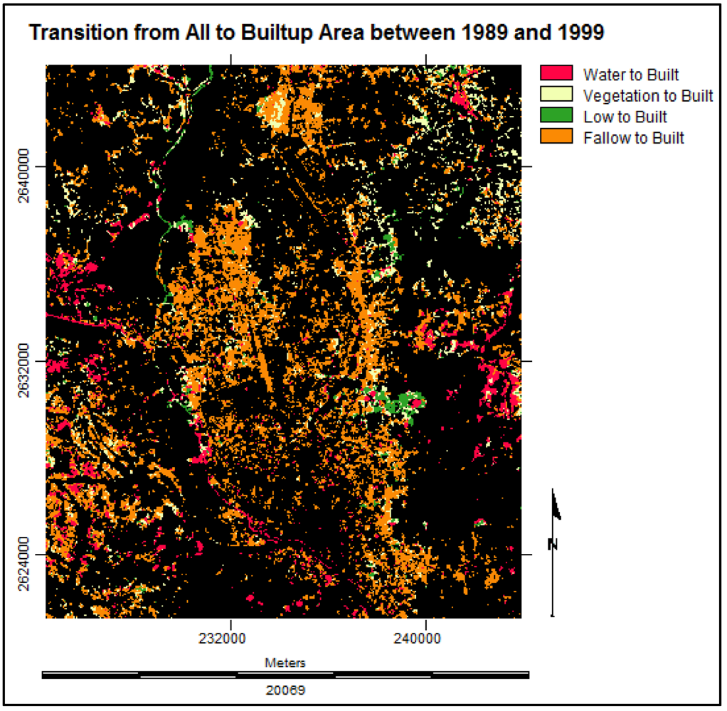
3.1. Land Cover Change Detection Analysis
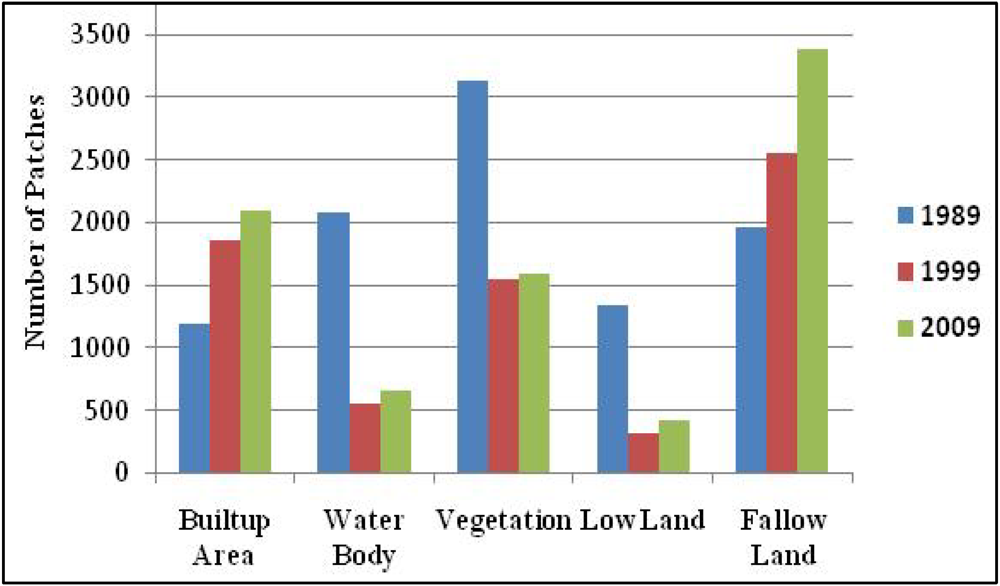
3.1.1. Number of Patches (NP)

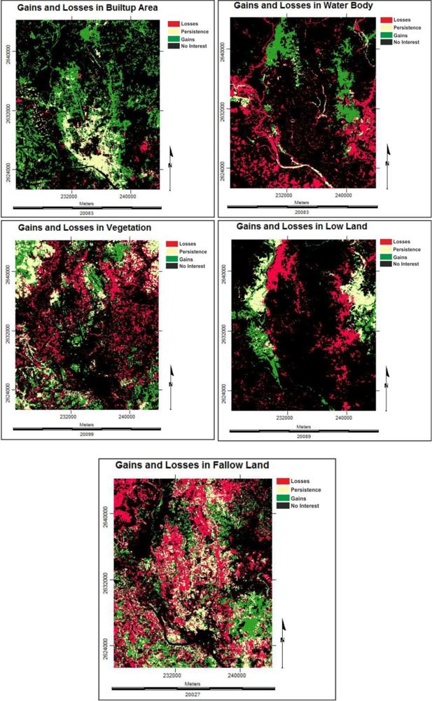
3.1.2. Gains and Losses in Land Cover Types

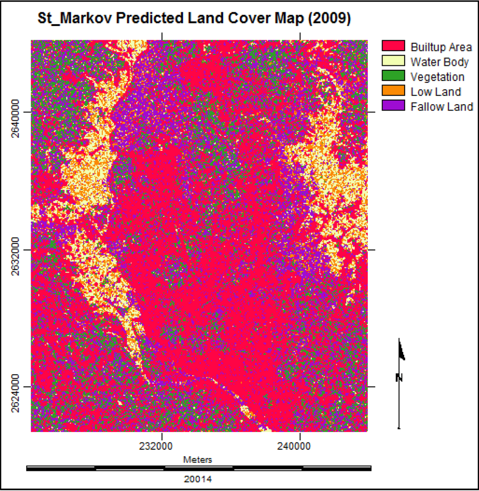
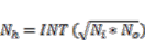
3.2. Stochastic Markov Model
3.2.1. Markov Property
 (1)
(1) (2)
(2) (3)
(3)3.2.2. Transition Matrix for a Markov Chain
 (4)
(4) (5)
(5) =
=  ∙Pt (7)
3.2.3. Analysis with Stochastic Markov Model
| Built-up Area | Water Body | Vegetation | Low Land | Fallow Land | |
|---|---|---|---|---|---|
| Built-up Area | 0.6649 | 0.0268 | 0.0533 | 0.0298 | 0.2252 |
| Water Body | 0.2125 | 0.1074 | 0.1030 | 0.1969 | 0.3802 |
| Vegetation | 0.1675 | 0.0853 | 0.3304 | 0.1173 | 0.2995 |
| Low Land | 0.0766 | 0.4006 | 0.0514 | 0.3446 | 0.1267 |
| Fallow Land | 0.4126 | 0.0144 | 0.2603 | 0.0199 | 0.2928 |
| Built-up Area | Water Body | Vegetation | Low Land | Fallow Land | |
|---|---|---|---|---|---|
| Built-up Area | 95,476 | 3,845 | 7,658 | 4,278 | 32,332 |
| Water Body | 10,034 | 5,074 | 4,865 | 9,300 | 17,953 |
| Vegetation | 17,569 | 8,945 | 34,655 | 12,302 | 31,409 |
| Low Land | 4,574 | 23,914 | 3,070 | 20,572 | 7,566 |
| Fallow Land | 57,732 | 2,009 | 36,415 | 2,789 | 40,964 |
3.2.4. Future Prediction Using Stochastic Markov Model
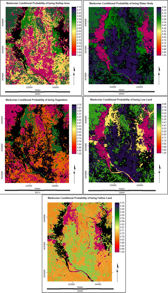
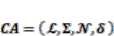
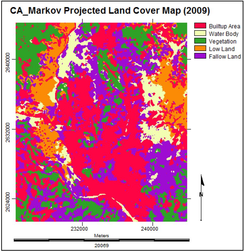
3.3. Cellular Automata Markov Model
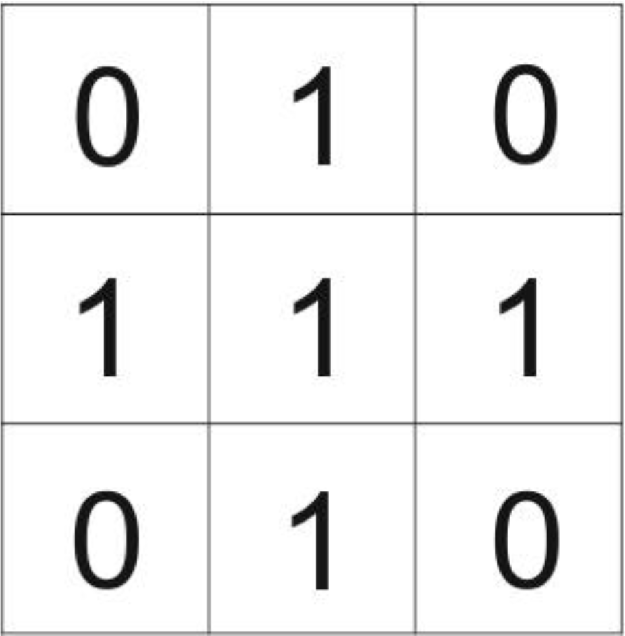
3.3.1. The Elements of Cellular Automata
- (a) The physical environment or the space represented by an array of cells, on which the automaton exists (its lattice).
- (b) The cell in which the automaton resides that contains its state(s).
- (c) The neighborhood around the automaton.
- (d) Transition rules that describe the behavior of the automaton.
- (e) The temporal space in which the automaton exists.
3.3.2. Mathematical Notation of Cellular Automata
 (8)
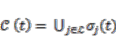
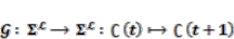
(8) ∑;
∑;  = the neighborhood of a cell automaton, which is defined as all cells that fall within a radius r around the actual cell. It denotes the idea of neighborhood template [24]:
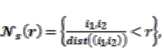 where
where 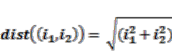 ;
;  = the relative index of all neighbors of a particular cell; δ = the local transition rule, which is denoted as follows [20]:
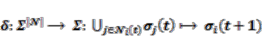 (9)i(t) = the associated neighborhood with ith cell at time t; | | = the number of cells in the neighborhood., the total number of possible rules equals [20]:
  (10)
(10) (11)
(11) (12)
(12) (13)
(13)3.3.3. Simulation with Cellular Automata Markov Model
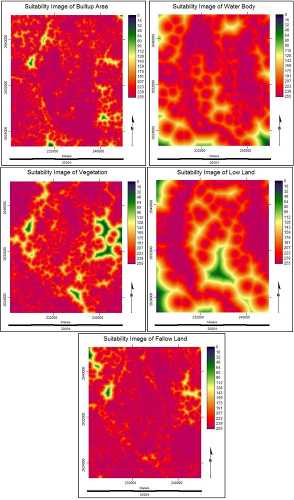
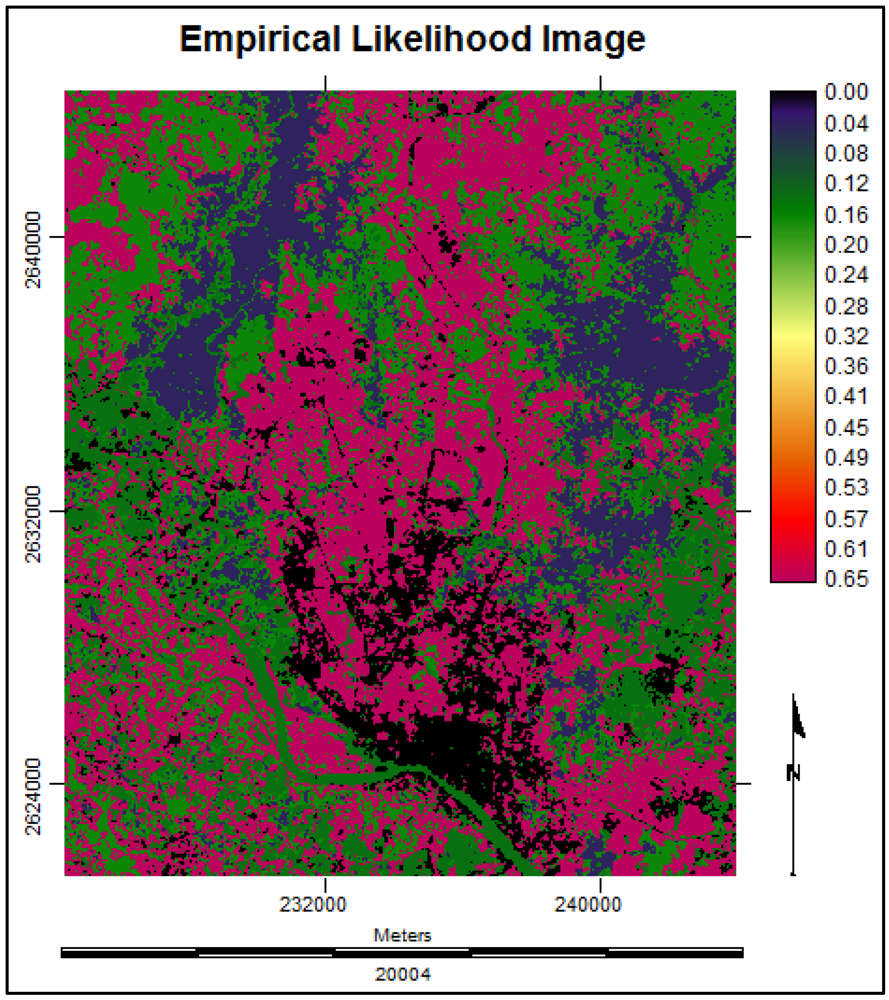
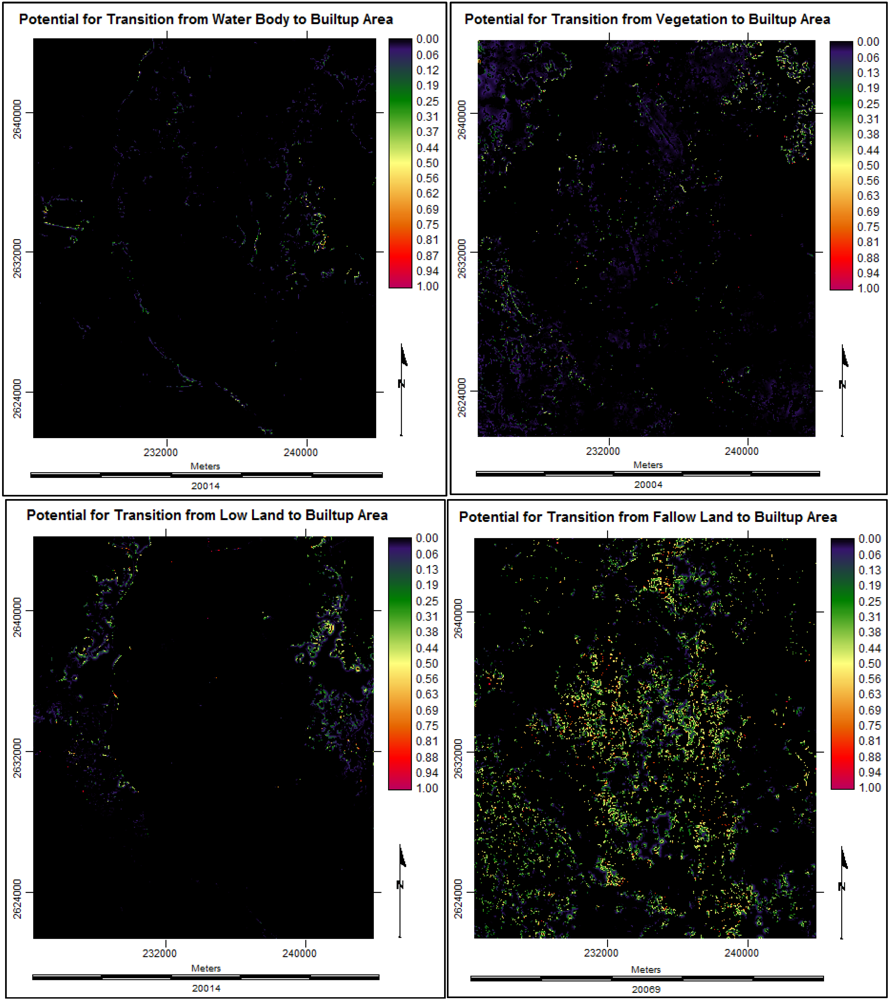
3.3.4. Suitability Maps for Land Cover Classes
3.3.5. Future Prediction Using Cellular Automata Markov Model
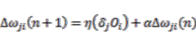
3.4. Multi Layer Perceptron Markov Model
3.4.1. The Feed-Forward Concept of Multi Layer Perceptron Neural Network
 (14)
(14) (15)
(15) (16)
(16)3.4.2. Number of Nodes
 (17)
(17)3.4.3. Number of Training Samples and Iterations
 (18)
(18)3.4.4. Multi Layer Perceptron Markov Modeling

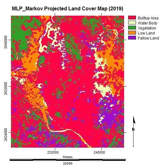
3.4.5. Future Prediction Using Multi Layer Perceptron Markov Model

| Built-up Area | Water Body | Vegetation | Low Land | Fallow Land | |
|---|---|---|---|---|---|
| Built-up Area | 0.7823 | 0.0174 | 0.0347 | 0.0194 | 0.1463 |
| Water Body | 0.2079 | 0.1264 | 0.1008 | 0.1927 | 0.3721 |
| Vegetation | 0.1529 | 0.0779 | 0.3887 | 0.1071 | 0.2734 |
| Low Land | 0.0695 | 0.3634 | 0.0467 | 0.4054 | 0.1150 |
| Fallow Land | 0.3825 | 0.0133 | 0.2413 | 0.0185 | 0.3445 |
3.5. Model Validation and Selection
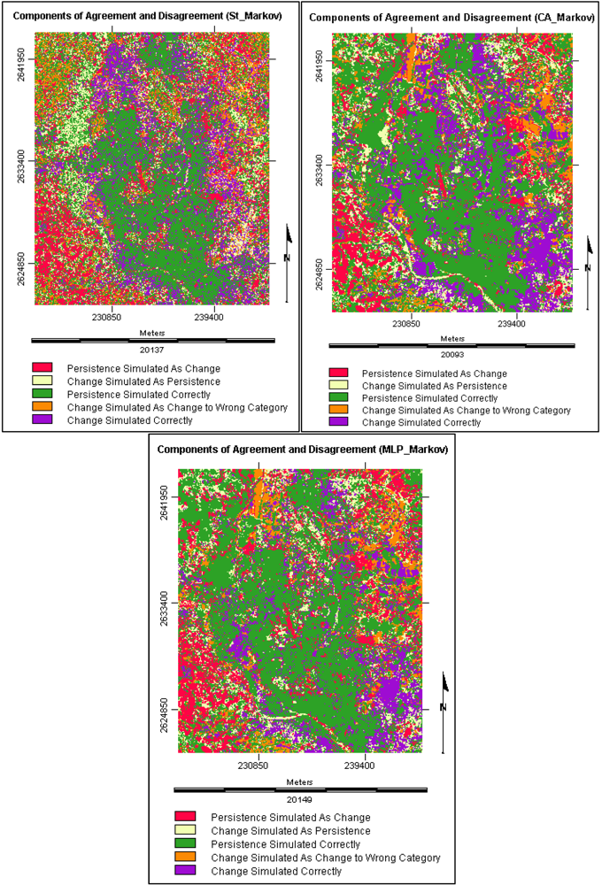
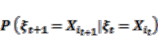
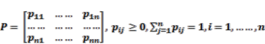
3.5.1. Components of Agreement and Disagreement
3.5.2. Validation Results
| Name of Component | St_Markov (%) | CA_Markov(%) | MLP_Markov (%) |
|---|---|---|---|
| Persistence Simulated Correctly | 44.424 | 48.459 | 50.578 |
| Change Simulated Correctly | 18.003 | 19.196 | 21.356 |
| Total Agreement | 62.427 | 67.655 | 71.934 |
| Change Simulated As Persistence | 11.369 | 10.39 | 9.788 |
| Persistence Simulated As Change | 16.736 | 13.54 | 10.751 |
| Change Simulated As Change to Wrong Category | 9.468 | 8.415 | 7.527 |
| Total Disagreement | 37.573 | 32.345 | 28.066 |
| Name of Component | St_Markov | CA_Markov | MLP_Markov |
|---|---|---|---|
| Temporal Dependency | √ | √ | √ |
| Spatial Dependency | × | √ | √ |
| Spatial Distribution | × | √ | √ |
| Spatial Proximity | × | √ | √ |
| Suitability Analysis | × | √ | √ |
| Transfer Function | × | × | √ |
| Weights of the Connections | × | × | √ |
| Training/ Testing Accuracy Assessment | × | × | √ |
| Transition Potential Maps | × | × | √ |

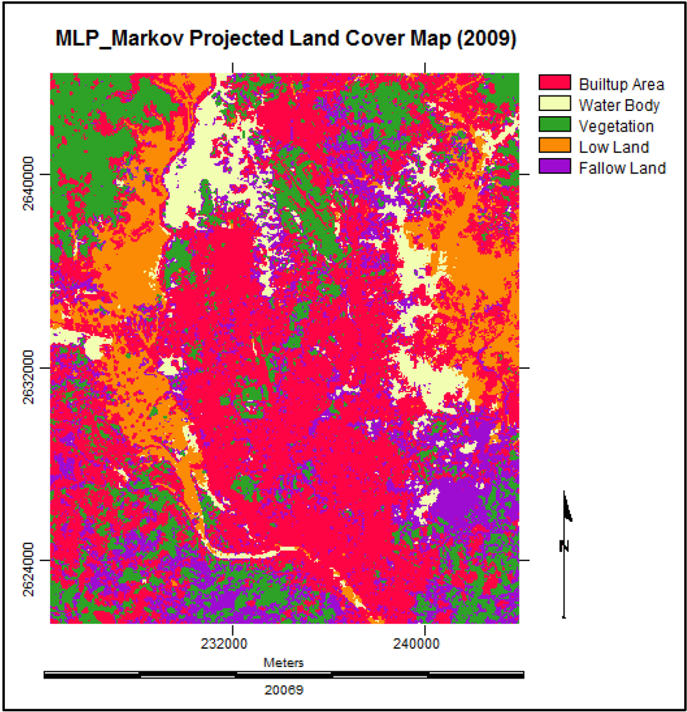
3.6. Simulating the Land Cover Map of 2019
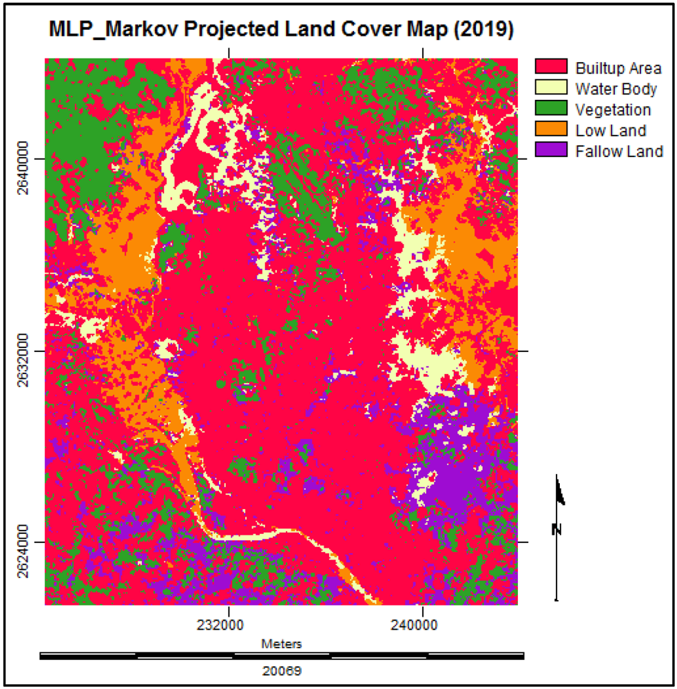
3.7. Analysis of the Final Predicted Map (2019)
4. Conclusions
Acknowledgments
References
- Khan, N.S. Temporal mapping and spatial analysis of land transformation due to urbanization and its impact on surface water system: A case from Dhaka metropolitan area, Bangladesh. Int. Arch. Photogramm. Remote Sens. 2000, 33, 598–605. [Google Scholar]
- Lambin, E.F. Remote sensing and GIS analysis. In International Encyclopedia of the Social and Behavioral Sciences; Smelser, N.J., Baltes, P.B., Eds.; Pergamon: Oxford, UK, 2001; pp. 13150–13155. [Google Scholar]
- Griffiths, P.; Hostert, P.; Gruebner, O.; Linden, S.V.D. Mapping mega city growth with multi-sensor data. Remote Sens. Environ. 2010, 114, 426–439. [Google Scholar]
- Dewan, A.M.; Yamaguchi, Y. Land use and land cover change in greater Dhaka, Bangladesh: using remote sensing to promote sustainable urbanization. Appl. Geogr. 2009, 29, 390–401. [Google Scholar]
- Emch, M.; Peterson, M. Mangrove forest cover change in the Bangladesh Sundarbans from 1989 to 2000: A remote sensing approach. Geocarto Int. 2006, 21, 5–12. [Google Scholar]
- Kashem, M.S.B. Simulating Urban Growth Dynamics of Dhaka Metropolitan Area: Cellular Automata Based Approach. Master Thesis, Department of Urban and Regional Planning, Bangladesh University of Engineering and Technology (BUET), Dhaka, Bangladesh, 2008. [Google Scholar]
- Lahti, J. Modelling Urban Growth Using Cellular Automata: A Case Study of Sydney, Australia. Master Thesis, Geo-information Science and Earth Observation for Environmental Modelling and Management, International Institute for Geo-information Science and Earth Observation, Enschede, The Netherlands, 2008. [Google Scholar]
- Cabral1, P.; Zamyatin, A. Three Land Change Models for Urban Dynamics Analysis in Sintra-Cascais Area. In Proceedings of 1st EARSeL Workshop of the SIG Urban Remote Sensing, Humboldt-Universität zu Berlin, Germany, 2–3 March 2006.
- Wang, J.; Mountrakis, G. Developing a multi-network urbanization (MuNU) model: A case study of urban growth in Denver, Colorado. Int. J. GIS 2011, 25, 229–253. [Google Scholar]
- Cheng, J.; Masser, I. Urban growth pattern modeling: A case study of Wuhan City, PR China. Landscape Urban Plan. 2003, 62, 199–217. [Google Scholar]
- Ahmed, B.; Hasan, R.; Ahmad, S. A Case Study of the Morphological Change of Four Wards of Dhaka City over the Last 60 years (1947–2007). Bachelor Thesis, Department of Urban and Regional Planning, Bangladesh University of Engineering and Technology (BUET), Dhaka, Bangladesh, 2008. [Google Scholar]
- Eastman, J.R. IDRISI Taiga Guide to GIS and Image Processing; Manual Version 16.02; Clark Labs: Worcester, MA, USA, 2009. [Google Scholar]
- Congalton, R. A Review of assessing the accuracy of classifications of remotely sensed data. Remote Sens. Environ. 1991, 37, 35–46. [Google Scholar]
- The ERDAS IMAGINE 9.1. On-Line Help System, Leica Geosystems Geospatial Imaging, LLC: Norcross, GA, USA, 2006.
- Tewolde, M.G.; Cabral, P. Urban sprawl analysis and modeling in Asmara, Eritrea. Remote Sens. 2011, 3, 2148–2165. [Google Scholar]
- McGarigal, K.; Cushman, S.A.; Neel, M.C.; Ene, E. FRAGSTATS: Spatial Pattern Analysis Program for Categorical Maps; University of Massachusetts: Amherst, MA, USA, 2002. Available online: http://www.umass.edu/landeco/research/fragstats/fragstats.html (accessed on 1 August 2011).
- Basharin, G.P.; Langville, A.N.; Naumov, V.A. The life and work of A. A. Markov. Linear Algebra Appl. 2004, 386, 3–26. [Google Scholar] [CrossRef]
- Balzter, H. Markov chain models for vegetation dynamics. Ecol. Model. 2000, 126, 139–154. [Google Scholar]
- Weng, Q. Land use change analysis in the Zhujiang Delta of China using satellite remote sensing, GIS and stochastic modelling. J. Environ. Manage. 2002, 64, 273–284. [Google Scholar]
- Maerivoet, S.; Moor, B.D. Cellular automata models of road traffic. Phys. Rep. 2005, 419, 1–64. [Google Scholar]
- Malczewski, J. GIS-based land-use suitability analysis: A critical overview. Progr. Plan. 2004, 62, 3–65. [Google Scholar]
- Wolfram, S. Statistical mechanics of cellular automata. Rev. Mod. Phys. 1983, 55, 601–644. [Google Scholar]
- Barredo, J.I.; Kasanko, M.; McCormick, N.; Lavalle, C. Modelling dynamic spatial processes: Simulation of urban future scenarios through cellular automata. Landscape Urban Plan. 2003, 64, 145–160. [Google Scholar]
- Li, X.; Yeh, A.G.O. Modelling sustainable urban development by the integration of constrained cellular automata and GIS. Int. J. GIS 2000, 14, 131–152. [Google Scholar]
- Karul, C.; Soyupak, S. A comparison between neural network based and multiple regression models for chlorophyll-a estimation. In Ecological Informatics; Recknagel, F., Ed.; Springer: Berlin, Germany, 2006; pp. 309–323. [Google Scholar]
- Atkinson, P.M.; Tatnall, A.R.L. Introduction neural networks in remote sensing. Int. J. Remote Sens. 1997, 18, 699–709. [Google Scholar]
- Cramér, H. Methods of estimation. In Mathematical Methods of Statistics, 19th ed; Chapter 33, Princeton University Press: Princeton, NJ, USA, 1999; pp. 497–506. [Google Scholar]
- Pontius, R.G., Jr; Millones, M. Death to Kappa: Birth of quantity disagreement and allocation disagreement for accuracy assessment. Int. J. Remote Sens. 2011, 32, 4407–4429. [Google Scholar] [CrossRef]
- Chen, H.; Pontius, R.J., Jr. Diagnostic tools to evaluate a spatial land change projection along a gradient of an explanatory variable. Landscape Ecol. 2010, 25, 1319–1331. [Google Scholar]
- Pontius, R.G., Jr.; Peethambaram, S.; Castella, J.C. Comparison of three maps at multiple resolutions: a case study of land change simulation in Cho Don District, Vietna. Ann. Assoc. Am. Geogr. 2011, 101, 45–62. [Google Scholar]
© 2012 by the authors; licensee MDPI, Basel, Switzerland. This article is an open-access article distributed under the terms and conditions of the Creative Commons Attribution license (http://creativecommons.org/licenses/by/3.0/).
Share and Cite
Ahmed, B.; Ahmed, R. Modeling Urban Land Cover Growth Dynamics Using Multi‑Temporal Satellite Images: A Case Study of Dhaka, Bangladesh. ISPRS Int. J. Geo-Inf. 2012, 1, 3-31. https://doi.org/10.3390/ijgi1010003
Ahmed B, Ahmed R. Modeling Urban Land Cover Growth Dynamics Using Multi‑Temporal Satellite Images: A Case Study of Dhaka, Bangladesh. ISPRS International Journal of Geo-Information. 2012; 1(1):3-31. https://doi.org/10.3390/ijgi1010003
Chicago/Turabian StyleAhmed, Bayes, and Raquib Ahmed. 2012. "Modeling Urban Land Cover Growth Dynamics Using Multi‑Temporal Satellite Images: A Case Study of Dhaka, Bangladesh" ISPRS International Journal of Geo-Information 1, no. 1: 3-31. https://doi.org/10.3390/ijgi1010003