Article

Sparse in the Time Stabilization of a Bicycle Robot Model: Strategies for Event- and Self-Triggered Control Approaches

by
Joanna Zietkiewicz
1,*,
Dariusz Horla
1 and
Adam Owczarkowski
2
1
Faculty of Electrical Engineering, Institute of Control, Robotics and Computer Science, Poznan University of Technology, 60-965 Poznan, Poland
2
Reacto, os. Jagiellonskie 21, 61-229 Poznan, Poland
*
Author to whom correspondence should be addressed.
Robotics 2018, 7(4), 77; https://doi.org/10.3390/robotics7040077
Submission received: 13 October 2018 / Revised: 14 November 2018 / Accepted: 23 November 2018 / Published: 28 November 2018

Abstract

:
In this paper, the problems of event- and self-triggered control are studied for a nonlinear bicycle robot model. It has been shown that by applying control techniques based on triggering conditions, it is possible to reduce both state-based performance index, as well as the number of triggers, in comparison to a standard linear-quadratic control which consumes less energy of the control system and decreases the potential mechanical wear of the robot parts. The results presented in this paper open a new research field for further studies, as discussed in the Summary section, and form the basis for further research in energy-efficient control techniques for stabilizing a bicycle robot.

1. Introduction

The bicycle invented by Karl von Drais [1,2,3] operates in an upright unstable equilibrium point, just as many animals do, leading to its inverted pendulum-like structure. Such structures are usually underactuated, which in the case of vehicles makes riding them fun. However, when handicapped or elderly people use them, additional stabilization units are welcome.
Current applications of such units enable one to stop the bicycle from maintaining its balance without any external forces, for instance, by using reaction wheels (see, e.g., a satellite application [4]). The reaction momentum phenomena can be found in multiple situations (see [5,6,7]). Numerous control laws have been used to control the reaction wheel pendulum, such as sliding mode control [8], fuzzy logic control [9,10], linear control laws with the use of feedback linearization (FBL) [11], predictive control [12], and neural network control [13]. In this paper, we aim to extend this list from a self-triggered control approach.
Dealing with the control task of bicycles using a traditional approach, when the moment of forces is exerted on a handlebar, especially for low linear speeds, e.g., 1 m s , is troublesome. Stabilization by a reaction wheel is, however, independent of the speed of the bicycle (robot). There are widely applied solutions in single-track vehicles stabilization, such as that of Lit Motors Inc. [14], where stabilization is based on using moments of forces resulting from a gyroscopic effect exerted by two rotating masses with variable rotation axes, and of Honda Riding Assist [15], which enables stabilization of a motor by controlling its handlebar. The problem, still, is the energy efficiency of such control laws. In the current paper, self-triggered and event-triggered control approaches are considered, being active only at certain time instants, and are used to present the energy-efficient control laws of such a structure.
The considered bicycle robot model has the same equilibrium point as a usual bicycle and has been built and used for experimental tests in our previous work. In this paper, the authors present the next step in their research on the control of this mechanical structure. In previous papers, the authors performed 4DoF simulations [16] by introducing robustness into the linear-quadratic regulator (LQR) control scheme or by comparing different control strategies, e.g., LQR, LQI, and LMI-based LQR control in [17]. The results helped the authors to focus on problems with a lesser DoF to be concerned, e.g., by introducing robustness into LQR/LQI control laws with results based on experiments [18] and then by introducing feedback linearization to a simulation model [19], with an in-depth analysis of the impact of the initial conditions and the robustness parameter [20], and different linearization schemes [21]. In [22], the authors extended the results, referring to the best combination of control approaches at the research stage of [18] when feedback linearization was used, for possible actuator failure in order to represent the uncertainty introduced by the linearization of the robot model or by possible constraints imposed on the control signal.
The current challenge in control systems, especially those where sensor readings or actuator actions should be made only when necessary, is to preserve the control performance of the closed-loop systems. Since control loops no longer have at their disposal enough communication resources, these implementation aspects have become important. Two of the most important techniques that reduce occupation of the bandwidth to the minimum necessary level and, at the same time, allow for the reduction of control energy, exerting control signals only when needed, are event- and self-triggered control algorithms. In the first one, the state of the plant is continuously measured, and the triggering condition indicating when to act monitors the plant continuously. In the self-triggered system, there is a prediction mechanism available, defining when updates in control should be triggered.
The above is the reason why authors have decided to perform the next step in their studies to find an efficient way of modifying the formerly presented control laws in the bicycle robot research field. These control approaches seem most appealing from the viewpoint of the energy of the control signal, which, whenever changed, relates to the changing rotation velocity of the reaction wheel, requiring higher energy consumption.
The novelty of this paper is the application of the proposed control strategies to a single-track vehicle with a stabilization task, taking energy efficiency of the control law into account. The similar up-to-date approaches involve the stabilization of the motor by a gyroscopic effect by means of three rotating flywheels [14], the stabilization of motorcycles driving at a low speed by the automatic change in the rotation angle of the handlebar and the angle between the fork of the handlebar and the ground [15], or, in a less common approach, the stabilization of a cube on one of its corners [23]. No triggering approaches have been, to the best of the knowledge of the authors, applied to bicycle robot control tasks.
The paper presents simulation studies related to a nonlinear model developed, tested, and verified at multiple stages of previous experiments (see the above references). The paper is structured as follows: Section 2 introduces the mathematical model of the robot. Section 3 presents the considered control strategies that extend those considered hitherto. In Section 4, the experimental model is explained in brief, with a comparison of performances of the considered control strategies. Section 5 provides a summary.

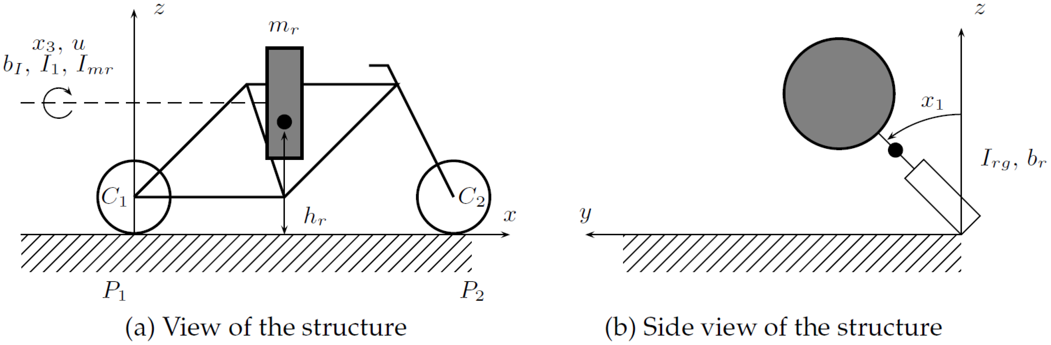
2. Mathematical Model of the Considered 2DoF Bicycle Robot Model

A two-degrees-of-freedom dynamic model [24] of the bicycle, taking the deflection angle from the vertical pose and the angle of rotation of the reaction wheel into account, is used in the form of an inverted pendulum. In addition, the authors have assumed that the handlebar is still, and centrifugal forces do not affect the whole structure. In this way, the actuator impact on the bicycle robot is studied for the considered control regime only.
The mathematical description of a 2DoF robot model is given by the following set of non-linear differential equations [19,20]:
x ˙ 1 ( t ) = x 2 ( t )
x ˙ 2 ( t ) = g h r m r sin x 1 ( t ) I r g b r x 2 ( t ) I r g + b I x 4 ( t ) I r g + k m u ( t ) I r g
x ˙ 3 ( t ) = x 4 ( t )
x ˙ 4 ( t ) = k m u ( t ) I I + I m r b I x 4 ( t ) I I + I m r
See Figure 1 for the kinematic scheme of the robot. The notation adopted in this paper is summarized in Table 1, and such forces as centrifugal, gravitation, and reaction momentum from the reaction wheel are taken into account with full reference to [25].
A basic friction model that assumes that the moment of the friction force is proportional to the angular velocity of the robot in a specific joint has been used. At this point of research, the main focus is on control techniques to use actuators effectively, not to verify the impact of the friction model on the use of a model.
In order to apply self- and event-triggered control strategies, the model has been linearized using the Jacobian matrix, such as in [16,18,21], to obtain x ̲ ˙ ( t ) = A J x ̲ ( t ) + b ̲ J u ( t ) , where
A J = 0 1 0 0 g h r m r I r g b r I r g 0 b I I r g 0 0 0 1 0 0 0 b I I I + I m r
b ̲ J = 0 k m I r g 0 k m I I + I m r
with the linearization point (units omitted) taken as x ̲ l = 0 ̲ .
Secondly, the linearized model has been discretized into the following form:
x ̲ t + 1 = A x ̲ t + b ̲ u t
y t = c ̲ T x ̲ t
by means of step-invariant discretization with the sampling period T S = 0.01 s . The output of the discrete-time model is y R , the constrained control signal u R , and the state vector x ̲ R n , and all are given in discrete time (denoted by subscript t, where t is a sample number referring to time instant t T S ), and c ̲ = [ 1 , 0 , 0 , 0 ] T .
The real robot, whosemodel has been considered in this paper, is presented in Figure 2 for illustrative purposes only. The current paper presents the early stage of research in the field, and, as in the previous work of the authors, simulation results are considered first to identify the most attractive control approach.
Parameters of the model with their descriptions are given in Table 2, with the current denoted as u ( t ) (i.e., the control input).
The implemented model has the same parameters as the real robot, which has been proved by numerous simulation vs. experimental results comparisons performed by the authors. At first, it is to be stressed that all parts of the robot have been initially weighed using a professional weight with the precision of ± 1 g . The moment of inertia (MOI) of the reaction wheel on the basis of its inner r 1 , its outer r 2 radii, height l, and mass density ρ has been evaluated on the basis of
I rw = ρ π l ( r 2 1 r 1 2 ) ( r 2 2 + r 1 2 ) 2 ,
and afterwards verified by the use of Autodesk Inventor software, which has a tool to estimate moments of inertia of rotating elements. The MOI of the motor has been obtained by modeling the rotor in Autodesk Inventor, again made of the same material as the real one, which in addition has been verified by means of calculating the moment of inertia of a rotating cylinder, with the diameter equal to the diameter of the rotor, measured by a precision caliper and weighed prior to that. The MOI of the robot relative to the ground has been obtained from Autodesk Inventor and verified by the Steiner formula to calculate moments of inertia for rotating masses with rotation axis shifted by a distance d. Distance from the ground to the centre of the mass has been obtained on the basis of
r ̲ 0 = k m k r ̲ k k m k ,
where r ̲ k represents the known locations of the centers of masses of the components of the robot (Autodesk), and m k represents their weighed masses. The gravity constant has been taken from physical tables, and the motor constant has been obtained on the basis of the specification of the motor (the moment of force equals the product of the motor constant and the motor current, and the nominal current and moment have been given in specification of the motor. The friction coefficient in the robot rotation has been estimated by a trial-and-error approach during real-world experiments. By means of improving the construction of the real robot, the friction effects have been minimized, and the coefficient has subsequently been selected by means of simulation to mimic the experimental results, related to angle delays in rotating joints of the robot. The same holds for the friction coefficient of the reaction wheel.
In addition, it has been assumed that the measurement of the output of the closed-loop system y ( t ) = x 1 ( t ) (see (8)) is subject to white noise with normal distribution, to reflect the real-world conditions.

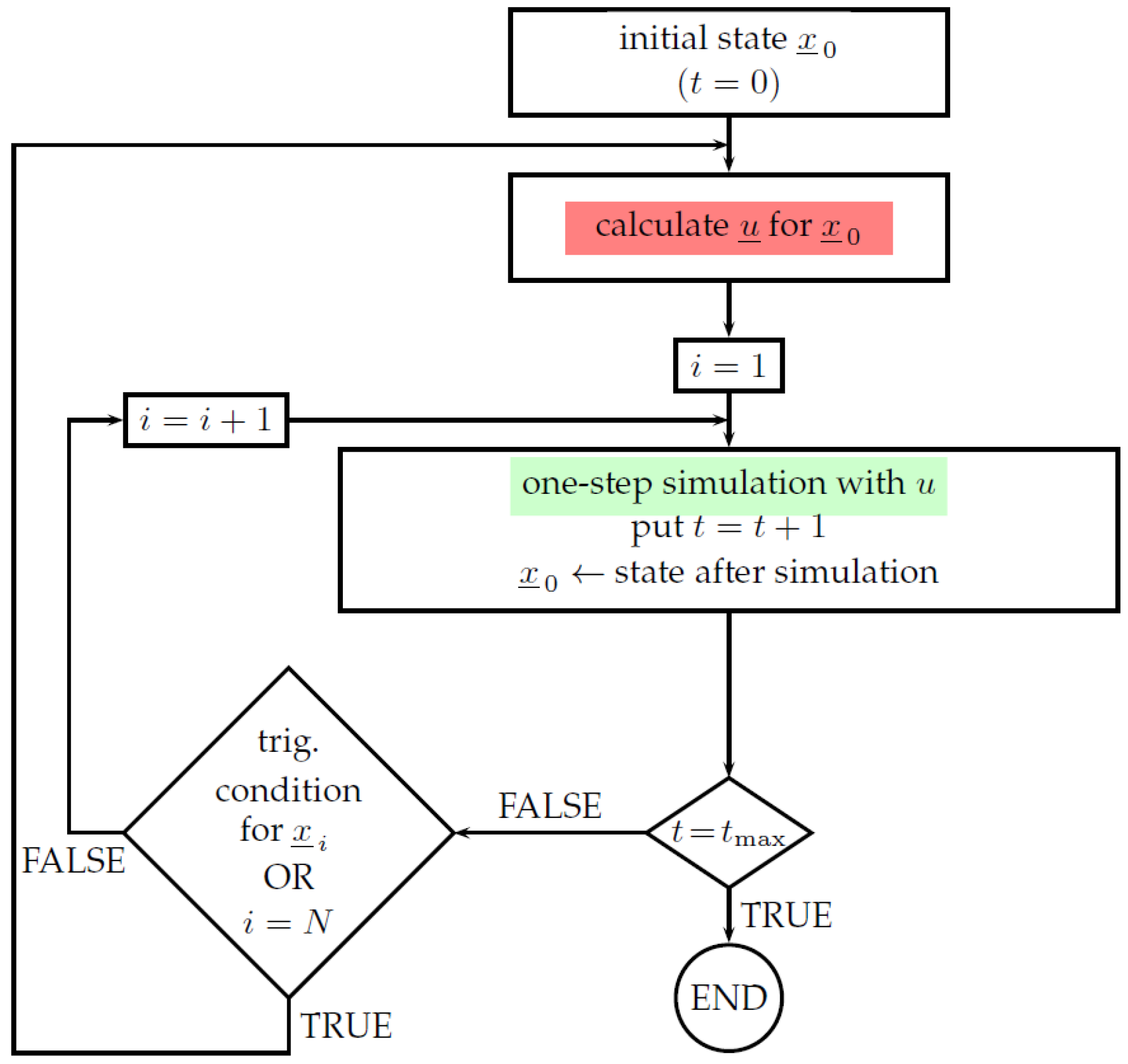
3. Considered Control Strategies

3.1. Introduction

Up to this point, as presented in the first section of this paper, the authors have focused on different linearization schemes applied to both discrete-time and continuous-time control techniques. This has led to identifying the most attractive control scheme [22], being at the same time energy-effective. Starting again from LQR approach the authors turn their attention now to triggered control techniques, which should allow to decrease both energy consumption (related to change in rotation of the reaction wheel), and at the same time reduce the mechanical wear of a robot. In order to satisfy this condition, three control techniques are considered, and finally compared, as presented in the following sections.

3.2. Preliminaries—Standard LQR Control

In this paper, three approaches are compared. As the reference point to all other considerations, the standard LQR control law of the form
u t = k ̲ T x ̲ t
is taken into account, where x ̲ t is the complete sampled state vector from the robot, originating from the nonlinear model of (1)–(4), which can be obtained from a full-state observer. This approach is presented here whenever a triggering parameter is taken as γ = 0 . The remaining control approaches are presented in the two following subsections.
The optimal vector k ̲ from (9) in a traditional approach is the solution for
k ̲ T = b ̲ T P b ̲ + R 1 b ̲ T P A
P = Q + A T P A A T P b ̲ b ̲ T P b ̲ + R 1 b ̲ T P A
where P > 0 is the solution to the Riccati equation, and appropriate vectors and matrices result from (7) and (8). and the performance index
J = t = 0 x ̲ t T Q x ̲ t + R u t 2 ,
with Q 0 , and R 0 as design criteria in the standard LQR approach.

3.3. The Event-Triggered Control Approach

Let us assume that x ̲ t is the most recently transmitted measurement of the full state of the nonlinear plant to the controller at sample t (at the same time, it can be obtained from a state observer on the basis of the separation principle [26]). Transmitting states to the controller, and the control update action, is based solely on triggering conditions. If a triggering condition is met, the state is transmitted to the controller, and the control u t sample is updated accordingly to the law of (9), to the form where x ̲ t : = x ̲ t . Otherwise, no state updates are transmitted, and the control action of (9) is not updated and is kept at a previously generated value. In this case, no calculations are needed, which reduces the computation burden, reduces the use of bandwidth, saves energy, etc.
According to [27,28], for the event-triggered system, the following triggering condition is used:
k ̲ T x ̲ t k ̲ T x ̲ t + l > γ k ̲ T x ̲ t + l
where γ > 0 can be related to a threshold value, and k ̲ is calculated on the basis of (10), (11), and l = 1 , 2 , (i.e., l grows until the condition of (13) is violated). This condition is related to a Lyapunov function.
If the condition (13) is met, the control signal is generated according to (9), where x ̲ t : = x ̲ t , updating the state x ̲ t , which corresponds now to the most recent measurement, accepted by the condition. In the other case, we simply move to the next sampling period, verifying (13) at the next sample hit. The value γ > 0 allows one to define the frequency of triggers and, at the same time, updates in the control signal, whereas for γ = 0 , and by supplying the state on the basis of the separation principle, a conventional LQR-type control is obtained.
The authors of [27] relate (13) to the quadratic event-triggering condition
z ̲ t + l T Γ z ̲ t + l > 0
where
z ̲ t + l = [ x ̲ t + l T , x ̲ t T ] T
Γ = ( 1 γ 2 ) k ̲ T k ̲ k ̲ T k ̲ k ̲ T k ̲ k ̲ T k ̲ .
In addition to (13), one can also assume the maximum number N of permissible sampling periods, after which a control update must take place. In this paper, it has been assumed that N = 10 .

3.4. The Self-Triggered Control Approach

In the case of event-triggered systems, the triggering condition is to be verified at all sampling instants, which requires additional computational power. In the self-triggered control approach, the control signal is updated whenever the sampling instant, calculated on the basis of, e.g., internal prediction and a triggering condition function, is satisfied, which requires the availability of the model of the plant.
In this approach, an altered method is inspired by [29,30,31], where the condition (13) is verified with respect to the prediction of x ̲ t + l made at sample t. This prediction, accompanied with the information about the next sample hit, is obtained from (7) and (8). To perform it, the control signal is assumed to be constant, and the first predicted sample of x ̲ t that violates the triggering condition yields the control update time instant.
Therefore, the triggering condition (13) for self-triggered control (STC) has the following form:
k ̲ T x ̲ t k ̲ T x ^ ̲ t + l > γ k ̲ T x ^ ̲ t + l
where x ^ ̲ t + l are predicted states x ̲ t + l with the use of the discrete model (7), i.e., according to
x ^ t + l = A l x ̲ t + A l 1 b ̲ A b ̲ b ̲ u t u t u t ,
where x ̲ t = x ̲ t and u t = k ̲ T x ̲ t .
The advantage of this approach is that there is no need to perform continuous measurements, and the actual state is measured whenever the control signal is updated, which improves energy-saving properties and reduces the occupation of the communication channel. A serious drawback, however, is that the prediction in this approach, is based on a linearized model.
It opens, though, a new field of research, taking different linearization schemes into account.

3.5. The Improved Self-Triggered Control Approach
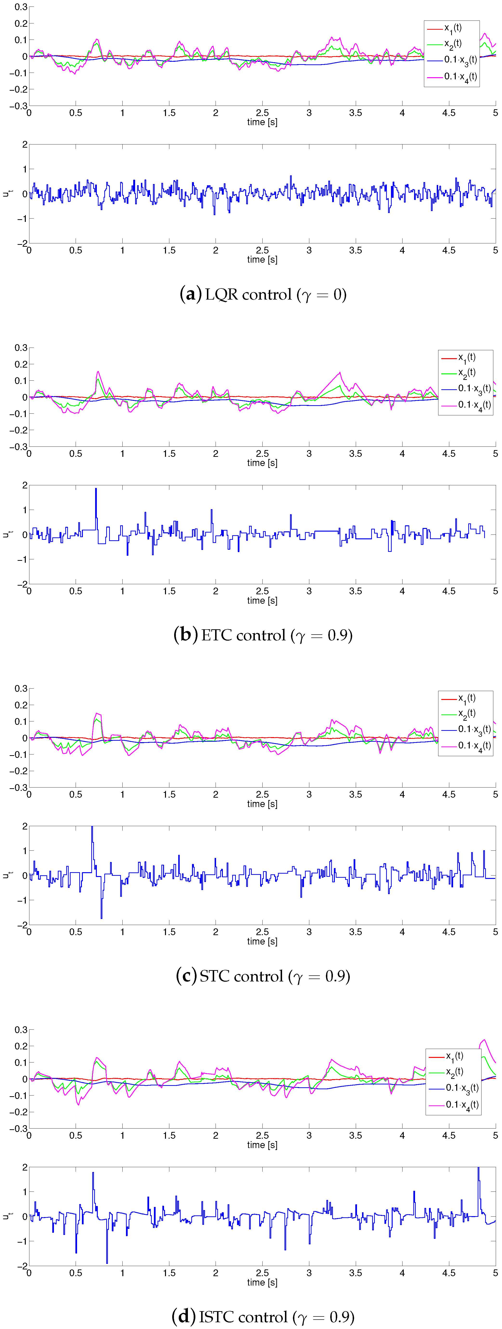
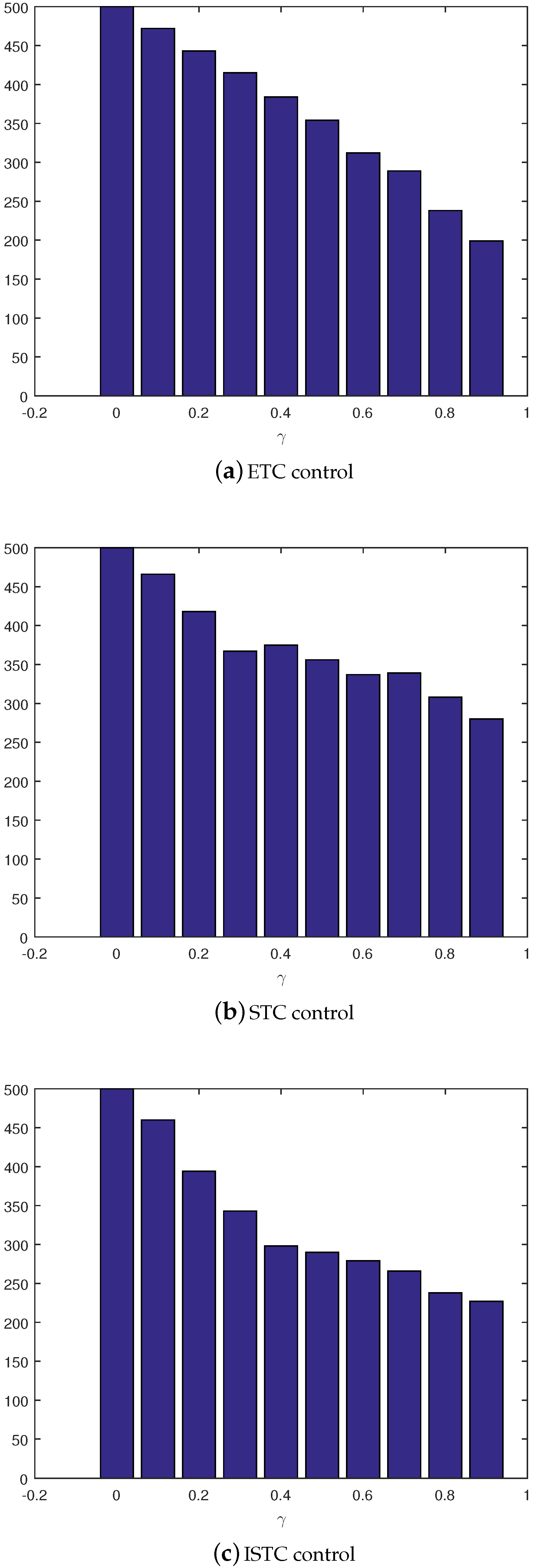
In this approach, it has been assumed that the prediction of the state x ̲ t is available at time instant t, and in order to calculate the control that suffices until the next x ̲ t , it is assumed that the state is used to compute samples of the control signal until x ̲ t appears. In this way, the control signal u t is constant no more but simply satisfies (9).
The triggering condition for ISTC is the same as for STC, (19), but now it is assumed that the input signal can change between triggers is constant. Therefore, the predictions of x ̲ t + l are calculated using the following model:
x ^ t + l = A l x ̲ t + A l 1 b ̲ A b ̲ b ̲ u t u t + 1 u t + l 2 u t + l 1 .
In addition, a cut-off constraint imposed on u t at the level of ± 2 A is taken into account, to mimic the real behavior of the robot controlled by the proposed scheme. Next, a complete state measurement is transmitted over the control channel, allowing one to calculate its prediction and improving the control quality, in comparison to standard STC. A similar approach is adopted in [32], where it is assumed that control signal samples are known between consecutive update instants.

4. Simulation Study

As in our previous paper [21], extensive simulation studies have been performed, to analyze and compare the three presented approaches, namely,
  • standard LQR control, where the following weighting matrices have been taken: Q = I 4 × 4 , R = 1 , and the control signal is updated at every step with sampling period T S = 0.01 s ,
  • event-triggered control, where it is assumed that the control update should be made no less than every 10 sampling periods, which forms an additional triggering condition, T S = 0.01 s , and
  • self-triggered control/improved-self triggered control based on prediction from the linearized model, where it is also assumed that control update should be made no less than every 10 sampling periods, T S = 0.01 s .
All the simulations have been performed for the following initial condition x ̲ ( 0 ) = [ 0 , 0 , 0 , 0 ] T (units omitted), and a noise sequence acting on x 1 .
A set of flowcharts, depicting the algorithms of event-triggered control (ETC), STC, and improved STC (ISTC) methods, respectively, has been included in Figure 3, Figure 4 and Figure 5, where red denotes LQR control (saturated) with a linear, continuous-time model, green denotes a nonlinear continuous-time model, and yellow denotes a linear discrete-time model for prediction purposes.
In Figure 6, a set of responses of closed-loop systems is presented, where for T S = 0.01 s the maximum number of triggers in the case of LQR control equals 500 (i.e., for γ = 0 ). As can be seen, all the considered control approaches yield in comparable control performance, resulting in proper stabilization of the bicycle robot model in an upright position. The difference is in the behavior of control signals, where, in the case of LQR control, a continuous update is visible, increasing control signal variance, leading to both the potential mechanical wear of the robot parts and the severe occupation of the communication channels. The remaining control approaches allow one to update the control signal less frequently, preserving the control performance at the same level.
In the case of the considered TC approaches, much less frequent update occurrences are visible, at the cost of more abrupt changes in control signals, which are smoothed in the case of the ISTC approach, in which velocity signals (i.e., states x 2 and x 4 ) are smoothed as a result of model-based updates in the control signal, spanned over several samples.
It is to be stressed that the considered methods need considerably fewer updates than the two other approaches to obtain similar responses, at the cost of more computations (as in a standard LQR control).
In Figure 7, the numbers of triggering events are presented for the considered control approaches, depicting an almost linear reduction trend for increasing γ in the case of ETC control, and a similar trend in the case of STC and ISTC control. It is visible that STC/ISTC require slightly more triggers in comparison to ETC, but this comes with the benefit of a less severe occupation of control channels, as the triggering condition is based on the model, not solely on the measurements, being a good alternative to the LQR approach requiring not only continuous measurement transmission but also 500 control updates in the considered control horizon, as shown in the simulations presented in this paper.
Finally, Figure 8 presents performance indices for the considered control strategies, stating that
I = 0 t max x ̲ ( t ) 2 d t
where t max is the simulation time. The presented performance index plot demonstrates the trade-off that potentially can be made between the closed-loop performance and the number of triggers in the corresponding control strategies.
Based on the results presented, it can be stated that the main point of application of the presented approach can be any control problem, where control updates are connected with additional energy consumption, unwanted transient behavior of the system, increased mechanical wear of the parts, or abrupt changes in signals, which should be avoided.

5. Summary and Future Work

In this paper, we aimed at providing an overview of possible control strategies that can potentially be used in the stabilization of a bicycle robot, taking the occurrences of an actuator use into account. The aim was not to cover all of the most up-to-date results, as this field in the last couple of years has expanded extensively, but to identify potentially interesting methods to perform a set of experiments on the bicycle robot. It has been shown that, despite the reduction in the frequency of control updates, it is still possible to stabilize the structure in the upright, unstable equilibrium point, increasing the energy efficiency of the control system.
The main point of this paper is to identify the control approach, which could be used most effectively on the real robot, as the authors did in their previous papers. According to the initial tests, the control algorithms proved to be effective, and the implementation on the real robot will be the matter for subsequent publications.
Up to this point, the STC or ETC mechanisms have been used for underactuated robots in the case of, e.g., an underwater robot [33], with no ISTC approach compared or verified. Tests of the application to bicycle robots have not yet been reported, to the best of the authors’ knowledge, though some papers are related to simple inverted pendulums in the form of event-triggered control [34] or to a linearized model of the pendulum and self-triggered control [35].
In all approaches, a Lyapunov function is applied to build a triggering condition, the function is widely used in ETC and STC approaches. The ETC approach from this paper is based on [27], and STC is inspired on [29,30,31], though the current paper uses a different prediction mechanism, which originates from using a different model. Here, we use a discrete-time model obtained from the linearization of the continuous-time nonlinear model at a point. In [32], it is remarked that there is no need to send control commands between consecutive triggers. Like the presented approach, the full control vector is sent. In their approach, however, the control is calculated for a continuous-time model, with subsequent control sampling.
In future work, we would also like to identify the impact of constraints imposed on the control signal, based on obtaining optimal control subject to control limits, to avoid implementing control using cut-off constraints only. One of the approaches to be considered might be the so-called tube MPC, and the STC control based on it. This could extend the result presented in [36] for linear systems to nonlinear plants, such as the bicycle robot itself, using, e.g., feedback linearization techniques, on the basis of our previous experience with the bicycle robot, especially [18,22]. In these papers, the feedback linearization approach allowed us to identify the conditions where control energy consumption is reduced by a visible amount, allowing one to maintain high control performance, despite constraints imposed on the current in the real robot.

Author Contributions

Conceptualization: J.Z., D.H. and A.O.; Methodology: J.Z. and D.H.; Software: J.Z.; Validation: J.Z., D.H. and A.O.; Formal analysis: J.Z. and D.H.; Investigation: D.H.; Resources: J.Z. and A.O.; Data curation: J.Z. and A.O.; Writing—original draft preparation: J.Z. and D.H.; Writing—review and editing: J.Z., D.H. and A.O.; Visualisation: J.Z. and D.H.; Supervision: J.Z. and D.H.; Project administration: D.H.

Funding

This research was financially supported as a statutory work of Poznan University of Technology (DSPB 04/45/DSPB/0184).

Conflicts of Interest

The authors declare no conflict of interest.

References

  1. Clayton, N. A Short History of the Bicycle; Amberley: Gloucestershire, UK, 2016. [Google Scholar]
  2. Hadland, T.; Lessing, H.E.; Clayton, N.; Sanderson, G.W. Bicycle Design: An Illustrated History; The MIT Press: Cambridge, MA, USA, 2014. [Google Scholar]
  3. Herlihy, D.V. Bicycle: The History; Yale University Press: New Haven, CT, USA, 2004. [Google Scholar]
  4. Tehrani, E.S.; Khorasani, K.; Tafazoli, S. Dynamic neural network-based estimator for fault diagnosis in reaction wheel actuator of satellite attitude control system. In Proceedings of the International Joint Conference on Neural Networks, Montreal, QC, Canada, 31 July–4 August 2005; pp. 2347–2352. [Google Scholar]
  5. Halliday, D.; Recnick, R.; Walker, J. Fundamentals of Physics Extended, 10th ed.; Wiley: Hoboken, NJ, USA, 2013. [Google Scholar]
  6. Acosta, V.; Cowan, C.L.; Graham, B.J. Essentials of Modern Physics; Harper & Row: New York, NY, USA, 1973. [Google Scholar]
  7. Norwood, J. Twentieth Century Physics; Prentice-Hall: Upper Saddle River, NJ, USA, 1976. [Google Scholar]
  8. Khalil, H.K. Nonlinear Systems, 3rd ed.; Prentice Hall: Upper Saddle River, NJ, USA, 2002. [Google Scholar]
  9. Bapiraju, B.; Srinivas, K.N.; Prem, P.; Behera, L. On balancing control strategies for a reaction wheel pendulum. In Proceedings of the IEEE INDICON, Khangapur, India, 20–24 December 2004; pp. 199–204. [Google Scholar]
  10. Gao, Q. Universal Fuzzy Controllers for Non-Affine Nonlinear Systems; Springer: Singapore, 2017. [Google Scholar]
  11. Fahimi, F. Autonomous Robots: Modeling, Path Planning, and Control; Springer: Berlin, Germany, 2008. [Google Scholar]
  12. Maciejowski, J.M. Predictive Control with Constraints; Prentice Hall: Upper Saddle River, NJ, USA, 2000. [Google Scholar]
  13. Miller, W.T., III; Sutton, R.S.; Werbos, P.J. Neural Networks for Control; MIT Press: Cambridge, UK, 1995. [Google Scholar]
  14. Carpenter, S. Lit Motors Hopes Its C-1 Becomes New Personal Transportation Option. Available online: http://www.latimes.com/business/autos/la-fi-motorcycle-car-20120526,0,4147294.story (accessed on 16 June 2012).
  15. Cameron, K. Honda Shows Self-Balancing but Non-Gyro Bike. Available online: https://www.cycleworld.com/honda-self-balancing-motorcycle-rider-assist-technology (accessed on 6 January 2017).
  16. Horla, D.; Owczarkowski, A. Robust LQR with actuator failure control strategies for 4DOF model of unmanned bicycle robot stabilised by inertial wheel. In Proceedings of the 15th International Conference IESM, Seville, Spain, 21–23 October 2015; pp. 998–1003. [Google Scholar]
  17. Owczarkowski, A.; Horla, D. A Comparison of Control Strategies for 4DoF Model of Unmanned Bicycle Robot Stabilised by Inertial Wheel. In Progress in Automation, Robotics and Measuring Techniques, Advances in Intelligent Systems and Computing; Roman, S., Ed.; Springer: Basel, Switzerland, 2015; pp. 211–221. [Google Scholar]
  18. Owczarkowski, A.; Horla, D. Robust LQR and LQI control with actuator failure of 2DoF unmanned bicycle robot stabilized by inertial wheel. Int. J. Appl. Math. Comput.Sci. 2016, 26, 325–334. [Google Scholar] [CrossRef]
  19. Zietkiewicz, J.; Horla, D.; Owczarkowski, A. Robust Actuator Fault-Tollerant LQR Control of Unmanned Bicycle Robot. A Feedback Linearization Approach; Challenges in Automation, Robotics and Measurement Techniqies; Szewczyk, R., Zieliński, C., Kaliczynska, M., Eds.; Springer: Berlin, Germany, 2016; pp. 411–421. [Google Scholar]
  20. Zietkiewicz, J.; Owczarkowski, A.; Horla, D. Performance of Feedback Linearization Based Control of Bicycle Robot in Consideration of Model Inaccuracy; Challenges in Automation, Robotics and Measurement Techniqies; Szewczyk, R., Zieliński, C., Kaliczynska, M., Eds.; Springer: Berlin, Germany, 2016; pp. 399–410. [Google Scholar]
  21. Horla, D.; Zietkiewicz, J.; Owczarkowski, A. Analysis of Feedback vs. Jacobian Linearization Approaches Applied to Robust LQR Control of 2DoF Bicycle Robot Model. In Proceedings of the 17th International Conference on Mechatronics, Prague, Czech Republic, 7–9 December 2016; pp. 285–290. [Google Scholar]
  22. Owczarkowski, A.; Horla, D.; Zietkiewicz, J. Introduction of feedback linearization to robust LQR and LQI control—Analysis of results from an unmanned bicycle robot with reaction wheel. Asian J. Control 2019, 21, 1–13. [Google Scholar] [CrossRef]
  23. Muehlebach, M.; D’Andrea, R. Nonlinear analysis and control of a reaction-wheel-based 3-D inverted pendulum. IEEE Trans. Control Syst. Technol. 2016, 25, 235–246. [Google Scholar] [CrossRef]
  24. Åström, K.J.; Klein, R.E.; Lennartsson, A. Bicycle dynamics and control: Adapted bicycles for education and research. IEEE Control Syst. 2005, 25, 26–47. [Google Scholar]
  25. Åström, K.J.; Block, D.J.; Spong, M.W. The Reaction Wheel Pendulum; Morgan & Claypool: San Rafael, CA, USA, 2007. [Google Scholar]
  26. Kwakernaak, H.; Sivan, R. Linear Optimal Control Systems; Wiley-Interscience: Hoboken, NJ, USA, 1972. [Google Scholar]
  27. Heemels, W.P.M.H.; Donkers, M.C.F.; Teel, A.R. Periodic Event-Triggered Control for Linear Systems. IEEE Trans. Autom. Control 2013, 58, 847–861. [Google Scholar] [CrossRef]
  28. Liu, T.; Jiang, Z.-P. Event-based control of nonlinear systems with partial state and output feedback. Automatica 2015, 53, 10–22. [Google Scholar] [CrossRef]
  29. Heemels, W.P.M.H.; Johansson, K.H.; Tabuda, P. An Introduction to Event-triggered and Self-triggered Control. In Proceedings of the 51st IEEE Conference on Decision and Control, Maui, HI, USA, 10–13 December 2012. [Google Scholar]
  30. Barradas Berglind, J.D.J.; Gommans, T.M.P.; Heemels, W.P.M.H. Self-triggered MPC for constrained linear systems and quadratic costs. In Proceedings of the 4th IFAC Nonlinear Model Predictive Control Conference, Noordwijkerhout, The Netherlands, 23–27 August 2012. [Google Scholar]
  31. Gommans, T.; Antunes, D.; Donkers, T.; Tabuda, P.; Heemels, M. Self-triggered linear quadratic control. Automatica 2014, 50, 1279–1287. [Google Scholar] [CrossRef]
  32. Wang, W.; Li, H.; Yan, W.; Shi, Y. Self-Triggered Distributed Model Predictive Control of Nonholonomic Systems. In Proceedings of the 11th Asian Control Conference, Gold Coast, Australia, 17–20 December 2017. [Google Scholar]
  33. Heshmati-Alamdari, S.; Eqtami, A.; Karras, G.C.; Dimarogonas, D.V.; Kyriakopoulos, K.J. A self-triggered visual servoing model predictive control scheme for under-actuated underwater robotic vehicles. In Proceedings of the 2014 IEEE International Conference on Robotics and Automation ICRA, Hong Kong, China, 31 May–5 June 2014; pp. 3826–3831. [Google Scholar]
  34. Durand, D.; Castellanos, F.G.; Marchand, N.; Sánchez, W.F.G. Event-Based Control of the Inverted Pendulum: Swing up and Stabilization. J. Control Eng. Appl. Inform. SRAIT 2013, 15, 96–104. [Google Scholar]
  35. Hashimoto, K.; Adachi, A.; Dimarogonas, D.V. Self-Triggered Model Predictive Control for Nonlinear Input-Affine Dynamical Systems via Adaptive Control Samples Selection. IEEE Trans. Autom. Control 2017, 62, 177–189. [Google Scholar] [CrossRef] [Green Version]
  36. Brunner, F.D.; Heemels, W.P.M.H. Robust Self-Triggered MPC for Constrained Linear Systems. In Proceedings of the European Control Conference, Strasbourg, France, 24–26 June 2014. [Google Scholar]
Figure 1. Kinematic scheme of the considered bicycle robot model.
Robotics 07 00077 g001
Figure 2. Schematic picture of the modeled robot [18].
Robotics 07 00077 g002
Figure 3. Flowchart of the event-triggered control (ETC) algorithm.
Robotics 07 00077 g003
Figure 4. Flowchart of the self-triggered control (STC) algorithm.
Robotics 07 00077 g004
Figure 5. Flowchart of the improved STC (ISTC) control algorithm.
Robotics 07 00077 g005
Figure 6. Considered control strategies—time responses.
Robotics 07 00077 g006
Figure 7. Considered control strategies—the number of triggers.
Robotics 07 00077 g007
Figure 8. Quality indices for considered control strategies.
Robotics 07 00077 g008
Table 1. Notation and nomenclature used in this paper.
SymbolMeaning
x ̲ R n state vector
x 1 [ rad ] vertical deflection angle of the robot
x 2 [ rad s ] angular velocity of the robot
x 3 [ rad ] angle of rotation of the reaction wheel
x 4 [ rad s ] angular velocity of the reaction wheel
u [ A ] R control signal (current of the motor)
m r [ kg ] weight of the robot
I I [ kg m 2 ] moment of inertia of the reaction wheel
I m r [ kg m 2 ] moment of inertia of the rotor of the motor
I r g [ kg m 2 ] moment of inertia of the robot (rel. to the ground)
h r [ m ] distance between the ground and the center of mass of the robot
g [ m s 2 ] gravity force
k m [ ] constant of the motor
b r [ ] friction coefficient in rotational movement
b I [ ] friction coefficient in the rotation of the reaction wheel
P 1 , P 2 contact points of the wheels with the ground
C 1 center of the rear wheel
C 2 center of the front wheel
LQRlinear-quadratic regulator
ETCevent-triggered control
STCself-triggered control
ISTCimproved self-triggered control
Table 2. Parameters of the unmanned bicycle robot.
ParameterValueDescription
m r 3.962 kg weight of the robot
I I 0.0094 kg m 2 moment of inertia (MOI) of the reaction wheel
I m r 0.001 kg m 2 MOI of the rotor
I r g 0.0931 kg m 2 MOI of the robot related to the ground
h r 0.13 m distance from the ground to the center of mass
g 9.8066 m s 2 gravity constant
k m 0.421 motor constant
b r 0.0001 friction coefficient in the robot rotation
b I 0.0001 friction coefficient of the reaction wheel

