Vibration Measurement in High Precision for Flexible Structure Based on Microscopic Vision

Abstract

Vibration measurement for flexible structures is widely used in various kinds of precision engineering fields. However, it is a challenge to measure vibration in special applications, such as cryogenic, dangerous and magnetic interference. In this paper, a high-precision vibration measurement system based on machine vision is designed. The circle center on the target is employed as the image feature. The circle feature is extracted using the improved algorithm based on gradient Hough transform. Then the image Jacobian matrix is used to compute the vibrations in Cartesian space from the image feature changes. Experiments verify the effectiveness of the proposed methods.

1. Introduction

Flexible structures are widely used in various kinds of precision engineering fields such as the cables of cable-stayed bridges [1,2], flexible inspection arms in international thermonuclear experimental reactors (ITER) [3], cryogenic targets used in inertial confinement fusion (ICF) [4], and spacecraft with solar panels [5]. As a type of fusion energy research, ICF attempts to initiate nuclear fusion reactions by heating and compressing a fuel target. The vibration of a cryogenic target causes many problems, such as the effectiveness of laser aiming and the target’s displacement. So the vibration measurement of a cryogenic target is an important research topic. The modal damping of those flexible structures is small. Once subjected to some kind of exciting force, its substantial vibration could continue for a long time. This will affect the equipment and also result in damage to the structure. So the vibration measurements of flexible structures play a crucial role in the prediction of potential disasters. A quite large number of monitoring techniques are available for structure vibration measurement. Among them, the most popular are probably the accelerometer-based measurements, the laser and the strain gages [6,7,8]. Although these techniques fit well for most applications, they present some limitations in special applications, such as cryogenic, strong electrical and magnetic interference. Vision-based vibration measurements have been studied by many researchers [9,10,11]. They can measure vibration displacements at multiple points simultaneously. These contactless vibration measuring techniques would be preferred in the special applications above.

In this paper, a vision system is presented to measure the vibration of a cryogenic target. The cryogenic target is mounted on a 3-DOF manipulator which is sealed in a closed cryogenic container. The developed system consists of two 1-DOF adjusting platforms, two microscopic cameras, and a computer. The techniques including the calibration of the image Jacobian matrix with active movements of the cryogenic target and the image feature extraction are presented. An improved adaptive Hough transform method is proposed to achieve the image feature extraction. The process of vibration measurement consists of three steps: (1) the image Jacobian matrix is calibrated before vibration measurement; (2) the coordinates of the target center are calculated via image feature extraction; (3) the vibrations in Cartesian space are computed from the image feature changes using the image Jacobian matrix. The vibration curve of the cryogenic target in the developed system can be automatically obtained in real time.

The rest of this paper is organized as follows. Section 2 gives a brief introduction of the system setup. In Section 3, the calibration of the image Jacobian matrix is provided. In Section 4, the autofocusing method is described. The image feature extraction based on an improved gradient Hough transform method is given. The vibration calculation is presented, too. Section 5 provides the experiments and results. Finally, this paper is concluded in Section 6.

2. System Setup

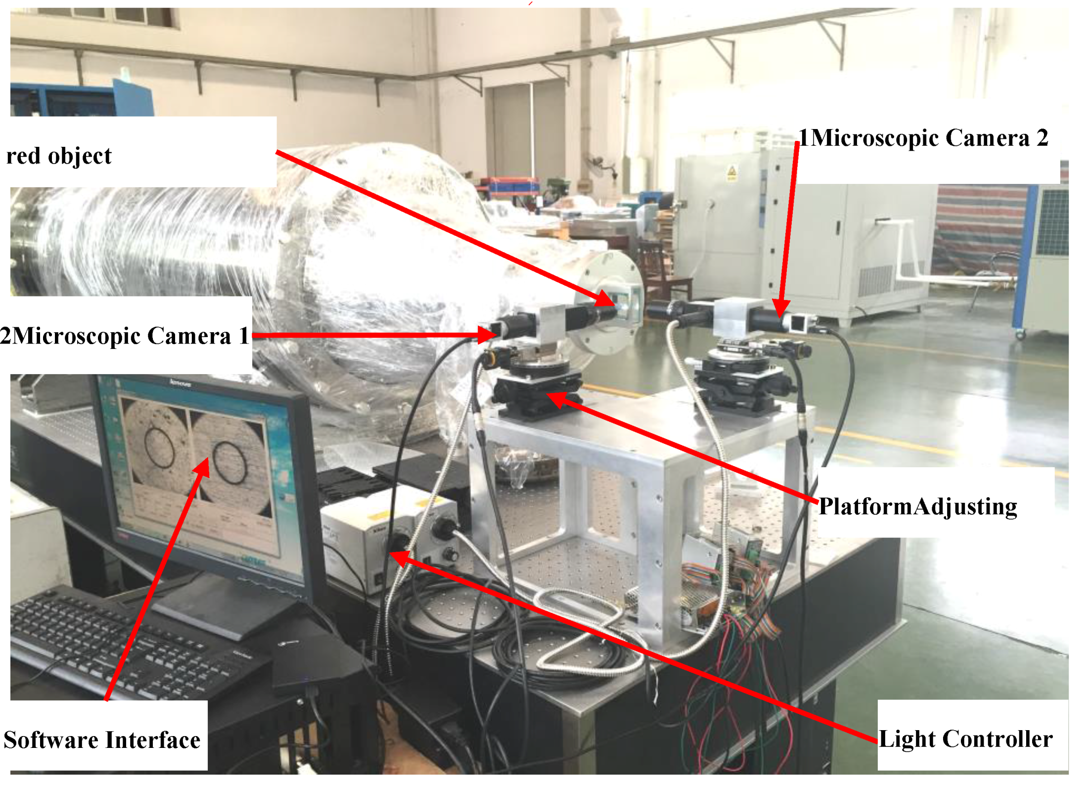
In the process of keeping a container cryogenic, the working of the cryocooler will lead to the target’s vibration. The vibration measurement system for the target is designed as given in Figure 1. It consists of two 1-DOF motion platforms, microscopic cameras, a light system and a computer. A microscopic camera and a motion platform with a support mechanism form a vision unit. The microscopic camera is formed with a microscope lens and a Charge-coupled Device (CCD) camera. The motion platform is employed to move the microscopic camera in order to adjust its distance to the object to be viewed. It has one translation DOF. The vision unit is mounted on the vibration isolation platform. The computer is used to capture images via the microscopic camera and to calculate the vibration of the cryogenic target.

The measured object is shown in Figure 1. It is a flexible structure object sealed in a cryogenic system. There is a circle at the end surface of the measured object, which is etched by the femtosecond laser. There are also circles at other surfaces. The external diameter of the circle is 500 μm. The measured object can be moved by a 3-DOF manipulator along the X_w-, Y_w- and Z_w-axis, respectively.

3. Calibration of Image Jacobian Matrix

In the microscopic vision system, the mapping from the plane of the clear view area to the image plane is linear because of the negligible lens distortion. The image Jacobian matrix can describe this mapping, which is the transformation matrix from the increments of the feature’s motion in the Cartesian space to the image feature changes [12,13]. The feature’s increments in the Cartesian space are the vibration to be measured. The image Jacobian matrix should be calibrated in advance in order to obtain the accurate vibration from the image feature changes. In this work, the target’s position is adjusted by the 3-DOF manipulator. Hence, the image Jacobian matrix can be calibrated via the active motion of the target.

Each microscopic camera is sensitive to 2-DOF translation. For example, microscopic camera 1 is sensitive to the translations along the Z_w- and Y_w-axis. Microscopic camera 2 is sensitive to the translations along the X_w- and Y_w-axis. The relation between the translation of the cryogenic target in Cartesian space and the feature changes on the images of two microscopic cameras can be expressed in Equation (1) if each feature point is chosen on the image of each microscopic camera.

$$\left[\begin{array}{l}\Delta u_{c1}\\ \Delta v_{c1}\\ \Delta u_{c2}\\ \Delta v_{c2}\end{array}\right]=\left[\begin{array}{lll}{J}_{11}\hfill & J_{12}\hfill & J_{13}\hfill \\ J_{21}\hfill & J_{22}\hfill & J_{23}\hfill \\ J_{31}\hfill & J_{32}\hfill & J_{33}\hfill \\ J_{41}\hfill & J_{42}\hfill & J_{43}\hfill \end{array}\right]\left[\begin{array}{c}\Delta x_m\\ \Delta y_m\\ \Delta z_m\end{array}\right]=J_{}\left[\begin{array}{c}\Delta x_m\\ \Delta y_m\\ \Delta z_m\end{array}\right]$$

(1)

where (Δu_c1, Δv_c1) and (Δu_c2, Δv_c2) are the two feature changes on the images of the two microscopic cameras, (Δx_m, Δy_m, Δz_m) is the incremental translation of the cryogenic target moved by the manipulator.

The relative positions of the cryogenic target in Cartesian and image space can be obtained for several active movements. Applying these data to the measuring model in Equation (1), an equation is formed.

$$\left[\begin{array}{cccc}\Delta u_{c11}& \Delta u_{c12}& \dots & \Delta u_{c1n}\\ \Delta v_{c11}& \Delta v_{c12}& \dots & \Delta v_{c1n}\\ \Delta u_{c21}& \Delta u_{c22}& \dots & \Delta u_{c2n}\\ \Delta v_{c21}& \Delta v_{c22}& \dots & \Delta v_{c2n}\end{array}\right]=\left[\begin{array}{lll}{J}_{11}\hfill & J_{12}\hfill & J_{13}\hfill \\ J_{21}\hfill & J_{22}\hfill & J_{23}\hfill \\ J_{31}\hfill & J_{32}\hfill & J_{33}\hfill \\ J_{41}\hfill & J_{42}\hfill & J_{43}\hfill \end{array}\right]\left[\begin{array}{cccc}\Delta x_1& \Delta x_2& \dots & \Delta x_n\\ \Delta y_1& \Delta y_2& \dots & \Delta y_n\\ \Delta z_1& \Delta z_2& \dots & \Delta z_n\end{array}\right]$$

(2)

where [Δx_i Δy_i Δz_i]^T is the relative position vector related to the reference in Cartesian space, [Δu_cji Δv_cji]^T is the relative image position vector related to the reference on the images of the j-th microscopic camera at i-th step active movement, and n is the step number of active motions, j = 1, 2.

Then the image Jacobian matrix can be solved from Equation (2) using the least squares method, as given in Equation (3).

$$J=A{B}^T{(B{B}^T)}^{-1}$$

(3)

where

$$\begin{gathered} J=\left[\begin{array}{lll}{J}_{11}\hfill & J_{12}\hfill & J_{13}\hfill \\ J_{21}\hfill & J_{22}\hfill & J_{23}\hfill \\ J_{31}\hfill & J_{32}\hfill & J_{33}\hfill \\ J_{41}\hfill & J_{42}\hfill & J_{43}\hfill \end{array}\right],A=\left[\begin{array}{cccc}\Delta u_{c11}& \Delta u_{c12}& \dots & \Delta u_{c1n}\\ \Delta v_{c11}& \Delta v_{c12}& \dots & \Delta v_{c1n}\\ \Delta u_{c21}& \Delta u_{c22}& \dots & \Delta u_{c2n}\\ \Delta v_{c21}& \Delta v_{c22}& \dots & \Delta v_{c2n}\end{array}\right] \\ B=\left[\begin{array}{cccc}\Delta x_1& \Delta x_2& \dots & \Delta x_n\\ \Delta y_1& \Delta y_2& \dots & \Delta y_n\\ \Delta z_1& \Delta z_2& \dots & \Delta z_n\end{array}\right] \end{gathered}$$

Therefore, once the feature changes on the images and the translation increments in Cartesian space with n steps of active movements are obtained, the image Jacobian matrix can be obtained with Equation (3).

4. Automated Measurement

The vibration measurement process mainly includes three parts: target autofocusing, feature extraction, and vibration measurement.

The image Jacobian matrix is calibrated in the initialization through several steps of active movements. The measuring apparatus is initialized by opening lighting sources and cameras. In the vibration measurement process, the clear images of the measured object can be captured by the two microscopic cameras through focus movement. In this work, there is a circle at the end surface of the measured object. When applied to other measurement objects, a specific shape target needs to be fixed at the surface of the measured object. Then, high-speed microscopic cameras record the video on the target vibration. The center coordinates of the target are extracted from the video captured by the two microscopic cameras. An improved gradient Hough transform algorithm is used to extract the circle center. Due to the large amount of image data acquisition, the image processing will take a long time which leads to a slow vibration measurement. In order to speed up the feature extraction, the method of the thread pool is used to synchronously calculate all the images in the captured video. The coordinate changes of feature points in adjacent frames are obtained, and then the actual amount of vibration can be calculated by the image Jacobian matrix. Finally, the displacement curve and the spectrum curve can be obtained, which are used to calculate the failure analysis information of the flexible structure.

4.1. Autofocus Strategy

During the vibration measurement process, the measured object should be on the clear imaging plane. Manual focusing is laborious and slow, and the repeatability precision is not ensured. So far, various autofocus techniques including focus evaluation functions [14,15] and focus searching algorithms [16] have been developed. Autofocus of the target is achieved by moving the microscopic camera along its optical axis. After autofocus of the target, the microscopic camera should stay fixed during the rest of the process. The focus evaluation function used in this work is the Sobel operator to enhance the importance of the edges.

$$J={\displaystyle \sum _{i=1}^M{\displaystyle \sum _{j=1}^{N}S(i,j)}}$$

(4)

where S(i, j) is the Sobel value of pixel (i, j). The size of the autofocus area is M × N. The focusing process is finished when the maximum value of Equation (4) is achieved in the predefined focusing range. When the image is clearest, the target is focused.

4.2. Feature Extraction

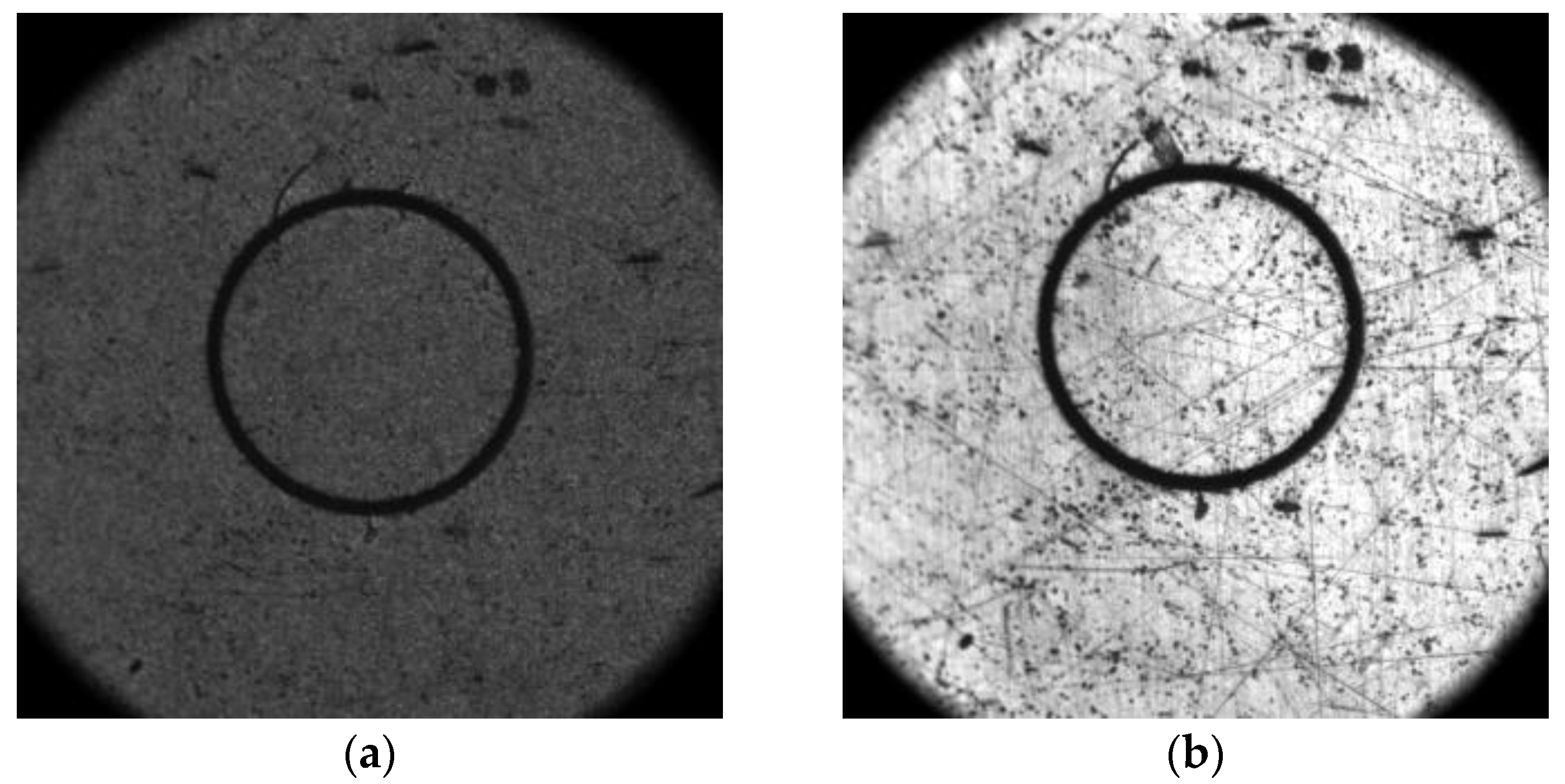
After the autofocus, the target video needs to be captured. All images in the video are processed to get the coordinates of the feature point. However, in our work, under different ultra-low temperature environments, the image of the target is inconsistent (see Figure 2). This is due to impure helium in the cryogenic vessel. It can cause the impurities attached to the target in different temperatures. This requires the algorithm to have good adaptability for different lighting environments. The image of the target has two circles (see Figure 2). The feature points are the centers of the two circles. The most popularly used algorithms for detecting circular patterns in an image are based on Hough transform. In this work, the gradient Hough transform algorithm [17,18] is used to detect the center of the target. The detection process of the target’s centers is as follows.

(1) The gradient field of image intensity is computed using the following Equation (5).

$$\{\begin{array}{l}{G}_x(i,j)=(f(i+1,j)-f(i,j)+f(i+1,j+1)-f(i,j+1))/2\hfill \\ G_y(i,j)=(f(i,j)-f(i,j+1)+f(i+1,j)-f(i+1,j+1))/2\hfill \end{array}$$

(5)

where (i, j) are the pixel indices, G_x(i, j) is the gradient vector in x direction at the pixel (i, j), G_y(i, j) is the gradient vector in y direction at the pixel (i, j), f(i, j) is the image intensity at the pixel (i, j).

The gradient directions of points on the circular pattern are either pointing towards the center of a circle or away from it. Based on this rule, the corresponding center coordinates of the circle can be obtained by the coordinates of the point on the circle and its gradient vector when the radius of the circle is fixed. The parameter space in Hough transform consists of the circle’s center and radius. So each point with a non-zero gradient vector is corresponding to a series of centers and radii. All points with a non-zero gradient vector are transformed to the center and radius space described by an accumulation array containing the different circle centers and radii. So, the elements’ values of the accumulation array are evaluated by a voting process similar to the standard Hough transform. The maximum value in the accumulation array gives the center and radius of a circle. The point whose gradient magnitude is less than the gradient filtering threshold G_T is not transformed in order to reduce the noise and improve the real-time performance. The values of G_T for different brightness images are manually given.

(2) In order to pinpoint the circle’s center, the centers corresponding to the elements with a larger value than the threshold in the accumulation array need to be filtered. The Laplacian of Gaussian (LoG) filter [19] is applied to give the area contour of the centers.

(3) The centroid of the area contour is calculated, which is taken as the accurate center of the circle.

4.3. Vibration Calculation

When the centers of the target’s circles in each image are extracted, the coordinate changes of center points in adjacent frames can be obtained. The actual amount of vibration can be calculated as

$$\begin{array}{l}\left[\begin{array}{c}\Delta x_{mk}\\ \Delta y_{mk}\\ \Delta z_{mk}\end{array}\right]={(J_{}^T{J}_{})}^{-1}{J}_{}^T\left[\begin{array}{c}\Delta u_{c1k}\\ \Delta v_{c1k}\\ \Delta u_{c2k}\\ \Delta v_{c2k}\end{array}\right]\end{array}$$

(6)

where (Δu_c1k, Δv_c1k) and (Δu_c2k, Δv_c2k) are the k-th increments of the two feature points on the images of the two microscopic cameras, and (Δx_mk, Δy_mk, Δz_mk) is the k-th translation increment of the cryogenic target.

Finally, the displacement curve and the spectrum curve can be obtained.

5. Experiments and Results

5.1. Experiment System

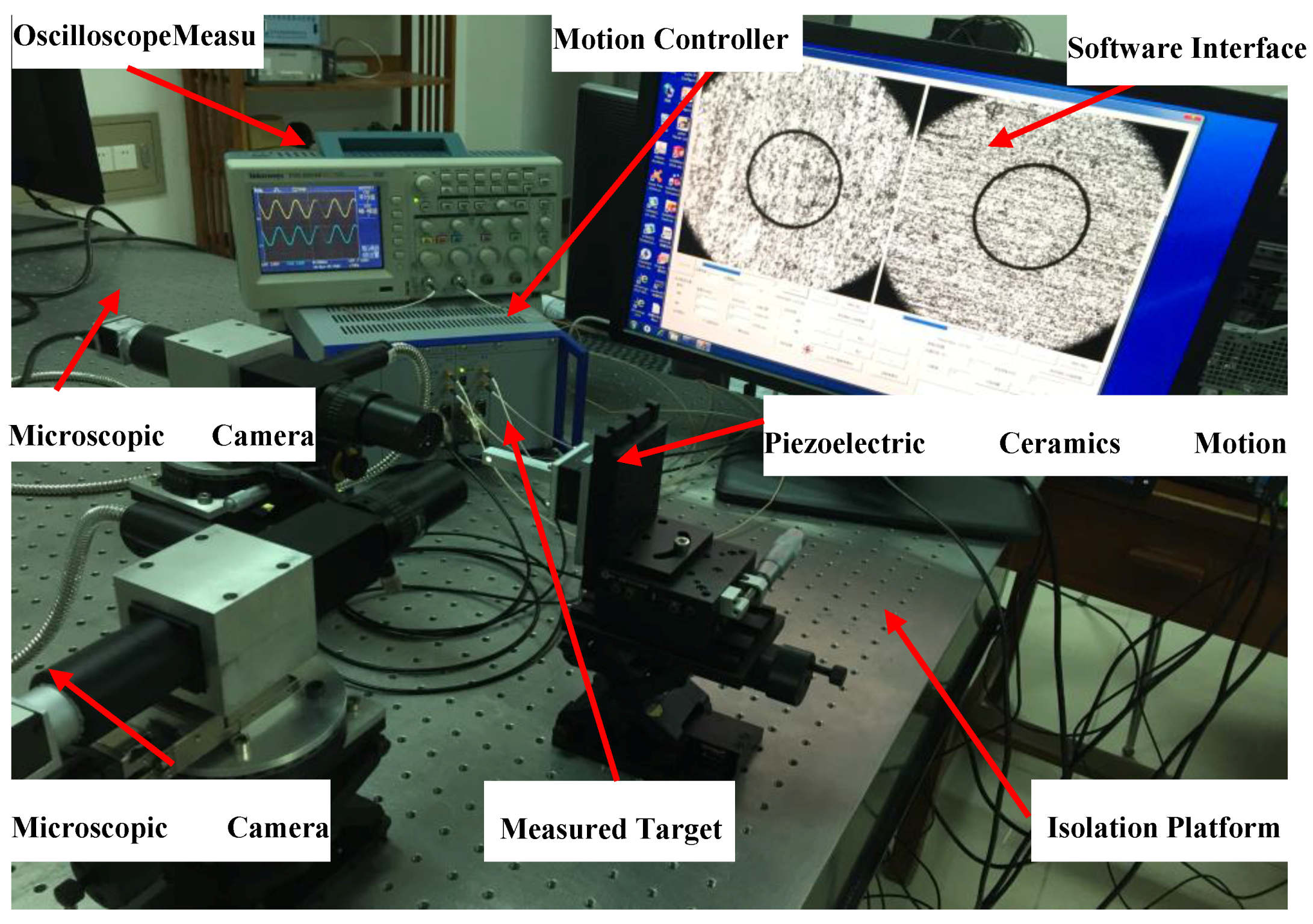
An experiment system was established according to the scheme given in Section 2, as shown in Figure 3. In this experiment system, both cameras are Basler cameras. Both cameras are equipped with Nikon zoom lenses with magnification of 10×, and they captured images at 90 frames per second with an image size of 2048 × 2048 pixels. The field-of-view dimensions of the two cameras were 1 mm × 1 mm. The two microscopic cameras were placed on Sigma SGSP26-50 to move along their optical axes. The translation resolution was 1 μm. The CPU of the host computer was Intel Core™2 DUO with a frequency of 2.8 GHz. The measurement accuracy in this system was 0.5 μm and the measurement vibration frequency range was 0–40 Hz.

5.2. Image Jacobian Matrixes Calibration

The manipulator actively translated the target with different distances as shown in matrix Mt, whose column was the increments of the target along the X_w-, Y_w- and Z_w-axis respectively. The increments were reasonably distributed around the origin. The extracted feature increments were recorded in matrix M_tc, whose column was the feature increments on images captured by the two microscopic cameras. Then the image Jacobian matrix J was computed in Equation (7). The pseudo-inverse of the Jacobian matrix was given in Equation (8).

$$M_t=\left[\begin{array}{cccccc}20& 0& 0& 0& 45& -13\\ 0& -20& 0& -40& 10& 25\\ 0& 0& 40& 0& -17& -25\end{array}\right]\mathsf{\mu }\text{m}$$

$$M_{tc}=\left[\begin{array}{cccccc}0.01& 2.01& 71.20& 4.82& -25.13& -37.20\\ 1.02& -32.50& 0.02& -67.60& 15.98& 40.60\\ 33.16& -4.87& 0.81& -6.43& 78.89& -25.48\\ 1.09& -32.47& 2.97& -67.51& 15.84& 40.65\end{array}\right] \text{pixel}$$

$$\begin{array}{l}{J}_{}=M_{tc}{M}_t^T{(M_t{M}_t^T)}^{-1}\\ =\left[\begin{array}{ccc}0.0351& -0.0339& 1.6682\\ 0.0041& 1.6665& 0.0163\\ 1.7597& 0.1290& 0.0815\\ 0.0102& 1.6801& 0.0689\end{array}\right]\end{array}$$

(7)

$${(J_{}^T{J}_{})}^{-1}{J}_{}^T=\left[\begin{array}{cccc}-0.0267& -0.0225& 0.5690& -0.0219\\ -0.0152& 0.2977& -0.0021& 0.2998\\ 0.5994& -0.0029& -0.0120& 0.0159\end{array}\right]$$

(8)

where M_t was the matrix formed by the active translation of the manipulator, M_tc was the matrix formed by the feature increments.

5.3. Feature Extraction

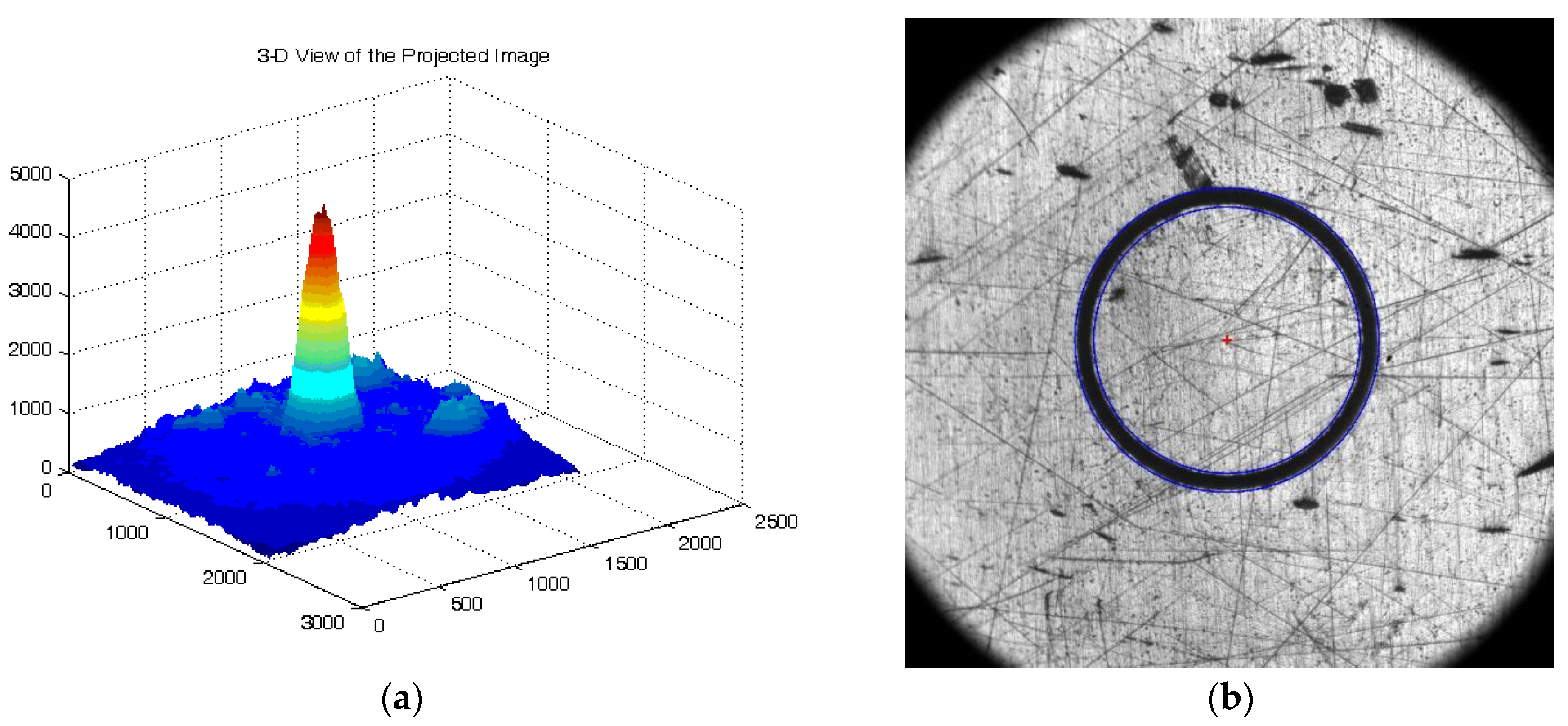
In the experiment of feature extraction, Figure 4a was the three-dimensional (3D) view of the accumulation array according to step (1) presented in Section 4.2. Figure 4b showed the detected result of the target. The point marked with “+” was the circle center. The circle marked with blue color was the contour of the target.

5.4. Offline Vibration Experiment

In the offline experiment, the vibration of the target was generated by a piezoelectric ceramics motion platform. An experiment system was established, which was shown in Figure 5. The sinusoidal signal was inputted in the piezoelectric ceramics motion platform for the vibration. The input vibration frequency was 1 Hz and the magnitude was 5 μm. The software interface was built by the virtual instrument Labview and an oscilloscope was used to verify the motion of the platform. In this work, the platform motion was controlled along the X_w- and Z_w-axis respectively. The frame rates of the cameras were set to 15 fps in actual measurements and the measured time was five seconds.

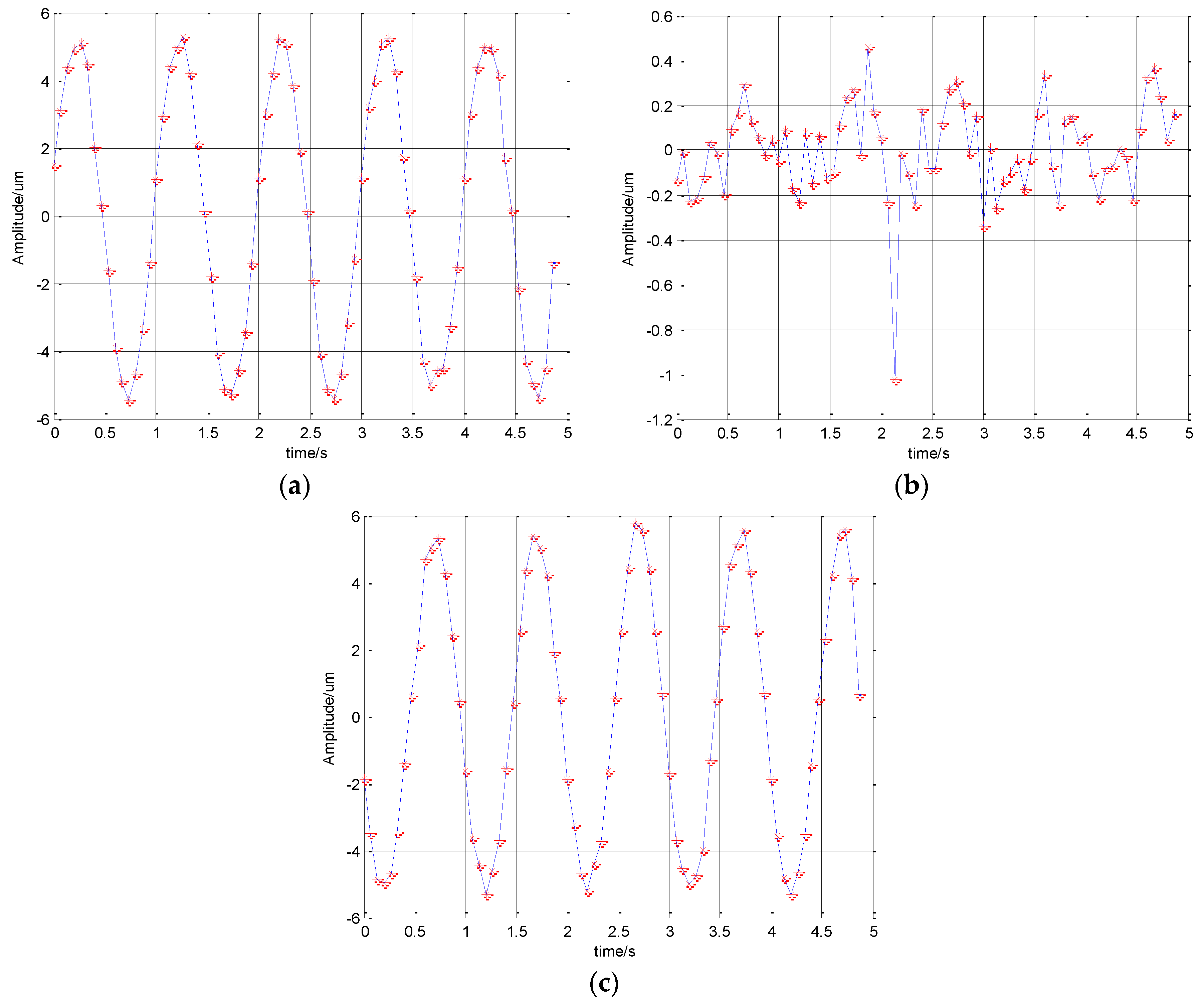
The measurement results were shown in Figure 6. It can be seen that the output of the displacement curves in the X_w and Z_w directions was the sinusoidal signal. The amplitude was 5 μm and the frequency was 1 Hz. The output result was consistent with the input vibration signal. Since there was no input in the Y_w direction, the maximum amount of vibration in the Y_w direction was less than 1 μm with disturbance from the external environment. The mean value of the vibration in the Y_w direction was −1.24 × 10⁻¹⁷ μm. The variance of the vibration in the Y_w direction was 4.48 × 10⁻². So, the proposed method was able to meet the measurement requirement.

5.5. Vibration Measurement

In the vibration measurement of the cryogenic target, the experiment system was established as shown in Figure 3. The vibration frequency we focused on was 0–40 Hz. Since the camera’s frame rate was 90 fps, the system was fully able to meet the measurement requirement according to the sampling theorem. However, when the displacement of the target in the camera exposure time was greater than one pixel equivalent in the high frequency vibration, it could result in blurred images of the target. In this case, we can use the information of the blurred images such as geometric moments to directly calculate the vibration amplitude [20,21,22,23,24].

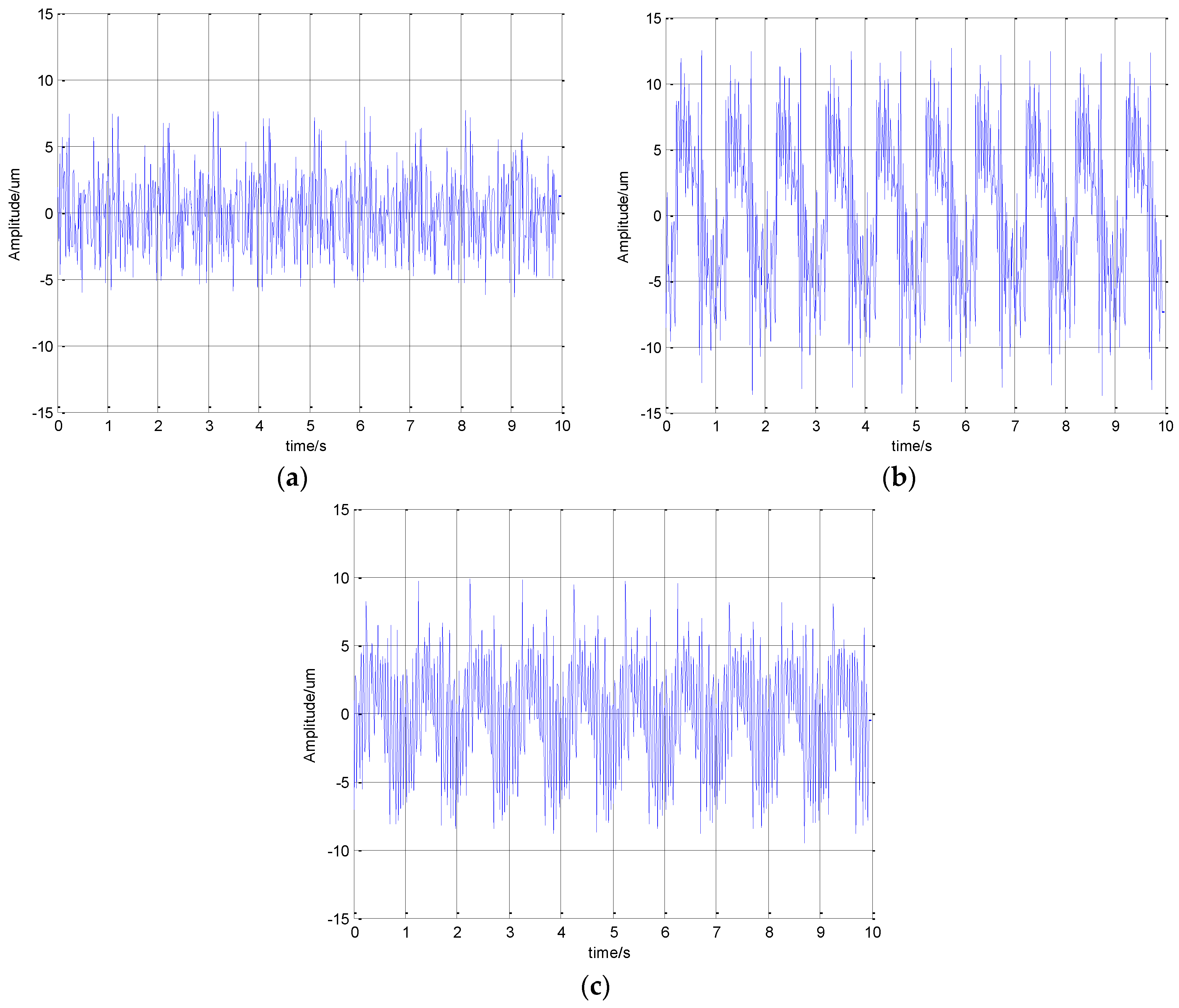
The measurement results were shown in Figure 7. The approximation of the μm/pixel scaling obtained by the pseudo-inverse of the Jacobian matrix in Equation (8) was 0.5 μm/pixel. As can be seen from Figure 7, the vibration amplitude in the Z_w and Y_w directions exceeded the amplitude in the X_w direction. The maximum amount of vibration in the Y_w direction reached 13 μm.

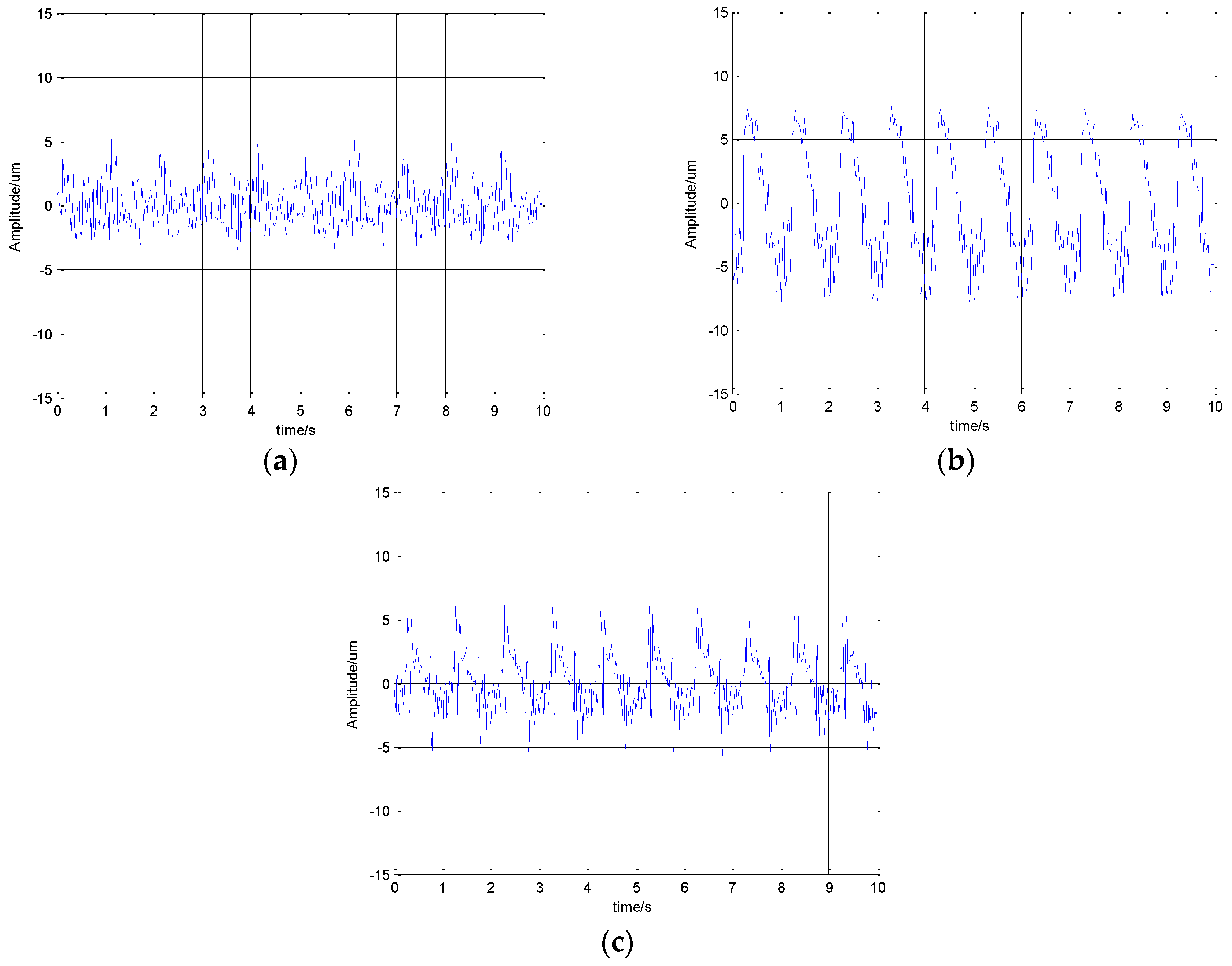
The Butterworth low-pass filter was used in this work to filter the high frequency vibration. The Butterworth filter was

$$G(z)=\frac{a_0+a_1{z}^{-1}+a_2{z}^{-2}+a_3{z}^{-3}+a_4{z}^{-4}}{b_0+b_1{z}^{-1}+b_2{z}^{-2}+b_3{z}^{-3}+b_4{z}^{-4}}$$

(9)

where a₀ = 9.3980851433795 × 10⁻², a₁ = 3.75923405735178 × 10⁻², a₂ = 0.563885108602767, a₃ = 0.375923405735178, a₄ = 9.3980851433795 × 10⁻², b₀ = 1, b₁ = 0, b₂ = 0.486028822068271, b₃ = 0, b₄ = 1.7664800872442 × 10⁻².

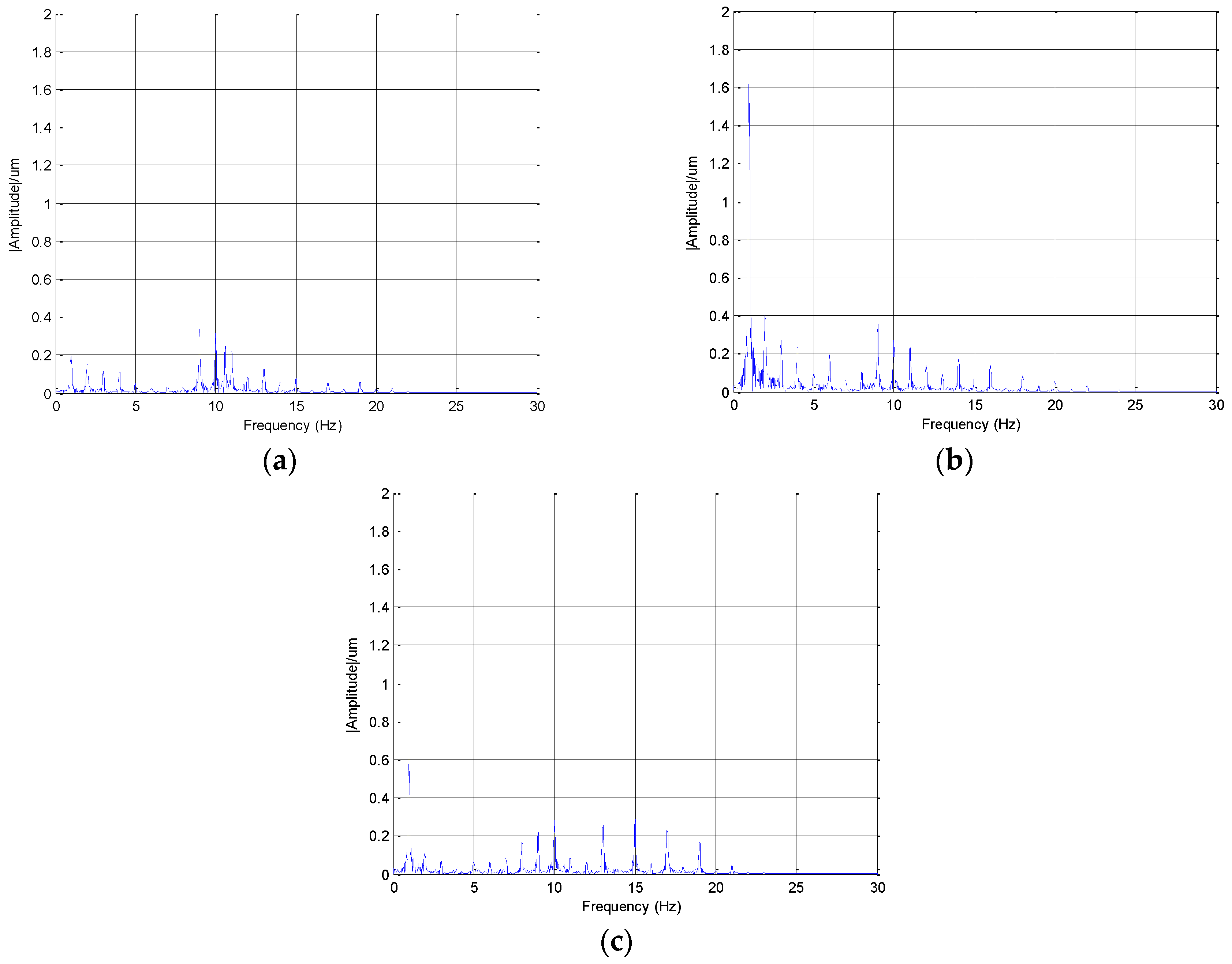
The measurement results after filtering were shown in Figure 8. The spectrum of the vibration experiment was shown in Figure 9. As can be seen from Figure 9, the frequency of 1 Hz in the Y_w direction was the main vibration frequency. The target reached the ultra-low temperature in the cryocooler. The main vibration of the target was from the cryocooler. The operating frequency of the cryocooler was 1 Hz. In Figure 9, many frequency components were visible in the spectra. Those vibration signals were from mechanical excitation generated by the control system of the target. These vibrations can be eliminated by the suppressing vibration bases. That vibration information can be used to calculate the vibration modes and failure analysis information of the measured object.

6. Conclusions

Our main contribution is that a precision vibration measurement instrument is designed for flexible structures. For high precision measurement, the image Jacobian matrix is applied for transforming the image feature changes to the vibrations in Cartesian space. The improved algorithm based on the gradient Hough transform algorithm is used for the feature extraction. Actual measurements verify the effectiveness of the proposed methods.

References

- Caetano, E.; Silva, S.; Bateira, J. A vision system for vibration monitoring of civil engineering structures. Exp. Tech. 2011, 35, 74–82. [Google Scholar] [CrossRef]
- Busca, G.; Cigada, A.; Manenti, A.; Zappa, E. Vision-based measurements for slender structures vibration monitoring. In Proceedings of the IEEE Workshop on Environmental, Energy, and Structural Monitoring Systems, Crema, Italy, 25 September 2009; pp. 98–102.
- Dubus, G.; David, O.; Measson, Y. A vision-based method for estimating vibrations of a flexible arm using on-line sinusoidal regression. In Proceedings of the IEEE International Conference on Robotics and Automation (ICRA), Anchorage, AK, USA, 3–7 May 2010; pp. 4068–4075.
- Ma, K.; Mei, L.; Liu, Y. Analysis and measurement of cryocooler vibration. High Power Laser Part. Beams 2013, 25, 637–639. [Google Scholar]
- Jiang, J.; Li, D. Dynamic Modeling and Modal Analysis of Smart Solar Array. Chin. Space Sci. Tech. 2008, 8, 32–38. [Google Scholar]
- Jin, Z.; Wu, J. Design of pipeline displacement detecting system based on MEMS accelerometer. Trans. Micros. Technol. 2012, 31, 140–145. [Google Scholar]
- Fu, Y.; Yang, C.; Xu, J.; Liu, H.; Yan, K.; Guo, M. Multi-point laser coherent detection system and its application on vibration measurement. SPIE Optical Metrology. In Proceedings of the International Society for Optics and Photonics, Munich, Germany, 21–22 June 2015.
- Dos Santos, F.L.M.; Peeters, B.; Lau, J.; Desmet, W.; Sandoval Goes, L.C. The use of strain gauges in vibration-based damage detection. J. Phys. Conf. Ser. 2015, 628, 012119. [Google Scholar] [CrossRef]
- Ribeiro, D.; Calçada, R.; Ferreira, J.; Martins, T. Non-contact measurement of the dynamic displacement of railway bridges using an advanced video-based system. Eng. Struct. 2014, 75, 164–180. [Google Scholar] [CrossRef]
- Son, K.S.; Jeon, H.S.; Park, J.H.; Park, J.W. A Technique for Vibration Measurement and Roundness Assessment of Rotating-axis using Camera Image. Trans. Korean Soc. Noise Vib. Eng. 2014, 24, 131–138. [Google Scholar] [CrossRef]
- Yao, J.; Xiao, X.; Liu, Y. Camera-based measurement for transverse vibrations of moving catenaries in mine hoists using digital image processing techniques. Meas. Sci. Tech. 2016, 27, 035003. [Google Scholar] [CrossRef]
- Xu, D.; Li, F.; Zhang, Z.; Shi, Y.; Li, H.; Zhang, D. Characteristic of monocular microscope vision and its application on assembly of micro-pipe and micro-sphere. In Proceedings of the 2013 32nd Chinese Control Conference (CCC), Xi’an, China, 26–28 July 2013; pp. 5758–5763.
- Li, F.; Xu, D.; Zhang, Z.; Shi, Y.; Shen, F. Pose measuring and aligning of a micro glass tube and a hole on the micro sphere. Int. J. Precis. Eng. Manuf. 2014, 15, 2483–2491. [Google Scholar] [CrossRef]
- Sun, Y.; Duthaler, S.; Nelson, B.J. Autofocusing algorithm selection in computer microscopy. In Proceedings of the 2005 IEEE/RSJ International Conference on Intelligent Robots and Systems, Edmonton, AB, Canada, 2–6 August 2005; pp. 70–76.
- Zong, G.; Sun, M.; Bi, S.; Yu, J. Research on auto-focus technique in micro-vision. Acta Opt. Sin. 2005, 25, 1225–1232. [Google Scholar]
- He, J.; Zhou, R.; Hong, Z. Modified fast climbing search auto-focus algorithm with adaptive step size searching technique for digital camera. IEEE Trans. Consum. Electron. 2003, 49, 257–262. [Google Scholar] [CrossRef]
- Peng, T.; Balijepalli, A.; Gupta, S.K.; LeBrun, T. Algorithms for on-line monitoring of micro spheres in an optical tweezers-based assembly cell. J. Comput. Inf. Sci. Eng. 2007, 7, 330–338. [Google Scholar] [CrossRef]
- Illingworth, J.; Kittler, J. The adaptive Hough Transform. IEEE Trans. Pattern Anal. 1987, 9, 690–698. [Google Scholar] [CrossRef]
- Shrivakshan, G.T.; Chandrasekar, C. A comparison of various edge detection techniques used in image processing. Int. J. Comp. Sci. Issues 2012, 9, 272–276. [Google Scholar]
- Zappa, E.; Matinmanesh, A.; Mazzoleni, P. Evaluation and Improvement of Digital Image Correlation Uncertainty in Dynamic Conditions. Opt. Lasers Eng. 2014, 59, 82–92. [Google Scholar] [CrossRef]
- Wang, S.; Guan, B.; Wang, G.; Li, Q. Measurement of sinusoidal vibration from motion blurred images. Pattern Recognit. Lett. 2007, 28, 1029–1040. [Google Scholar] [CrossRef]
- Guan, B.; Wang, S. The Amplitude Measurement of High-Frequency Vibration from Motion Blur Using Moments. J. Shanghai Jiaotong Univ. 2007, 41, 0447. (In Chinese) [Google Scholar]
- Zappa, E.; Mazzoleni, P.; Matinmanesh, A. Uncertainty assessment of digital image correlation method in dynamic applications. Opt. Lasers Eng. 2014, 56, 140–151. [Google Scholar] [CrossRef]
- Busca, G.; Ghislanzoni, G.; Zappa, E. Indexes for performance evaluation of cameras applied to dynamic measurements. Measurement 2014, 51, 182–196. [Google Scholar] [CrossRef]
© 2016 by the authors; licensee MDPI, Basel, Switzerland. This article is an open access article distributed under the terms and conditions of the Creative Commons by Attribution (CC-BY) license (http://creativecommons.org/licenses/by/4.0/).