On the Impact of Gravity Compensation on Reinforcement Learning in Goal-Reaching Tasks for Robotic Manipulators

1
Department of Electrical and Computer Engineering, University of Kentucky, Lexington, KY 40506, USA
2
Department of Mechanical Engineering, University of Kentucky, Lexington, KY 40506, USA
*
Authors to whom correspondence should be addressed.
Robotics 2021, 10(1), 46; https://doi.org/10.3390/robotics10010046
Submission received: 24 December 2020
/
Revised: 26 February 2021
/
Accepted: 1 March 2021
/
Published: 9 March 2021
Abstract
:Advances in machine learning technologies in recent years have facilitated developments in autonomous robotic systems. Designing these autonomous systems typically requires manually specified models of the robotic system and world when using classical control-based strategies, or time consuming and computationally expensive data-driven training when using learning-based strategies. Combination of classical control and learning-based strategies may mitigate both requirements. However, the performance of the combined control system is not obvious given that there are two separate controllers. This paper focuses on one such combination, which uses gravity-compensation together with reinforcement learning (RL). We present a study of the effects of gravity compensation on the performance of two reinforcement learning algorithms when solving reaching tasks using a simulated seven-degree-of-freedom robotic arm. The results of our study demonstrate that gravity compensation coupled with RL can reduce the training required in reaching tasks involving elevated target locations, but not all target locations.
1. Introduction
Autonomous robotic systems are widely recognized as a worthwhile technological goal for humanity to achieve. Autonomy requires solving a multitude of decision problems, from high level semantic reasoning [1] to low level continuous control input selection [2]. In this paper, we focus on continuous controller design for autonomous robot motion control. A typical controller takes in a feedback signal, containing state information, as well as a reference point and computes an actuation command. There are various ways to develop autonomous robotic control systems such as fuzzy logic [3,4], adaptive control [5,6], behavioral control theory [7,8], traditional robot control theory [2], inverse reinforcement learning [9,10], and reinforcement learning [11,12,13].
Control theory provides a methodology for creating controllers for dynamical systems in order to accomplish a specified task [14]. These methods are model-based, with the advantage that the performance of such controllers maybe characterized and even guaranteed before deployment. The use of models may be thought of as control based on indirect experience or knowledge. The limitation of model-based control approaches in robotic autonomy is the difficulty of obtaining accurate system models.
Reinforcement Learning (RL), in contrast to traditional robot control, aims to learn controllers from direct experience, and any knowledge gained thereof. Therefore, with RL, robots can learn novel behaviors even under changing environment. This is of great benefit for real world implementations. One example we can consider is brain machine interfaces (BMIs), which require real time adaptation of robot behaviors based on the user’s intention and changing environment [15,16]. However, approaches that use RL are, often intentionally, ignorant of the system dynamics and task. They learn controllers that complete a task through training and interacting with the task environment. One limitation of RL solutions to robotic autonomy is the large amount of interaction and training necessary to learn tasks. A limitation of model-based control approaches in robotic autonomy is the difficulty of obtaining accurate system models.
Due to the relative strengths and weaknesses of traditional robot control and reinforcement learning, researchers have worked on combining them to produce a controller design approach that overcomes their individual weaknesses. This combination broadly occurs in two forms, which may be thought of as series and parallel combination.
In a series combination, the reinforcement learning agent provide inputs to a low-level controller that is designed using traditional model-based approaches. The RL agent is in effect learning to tune gains or set-points, for example in [17]. The authors in [18] evaluate the impact of choosing various well-known traditional controllers. For tasks with kinematic constraints and contact rich environments, impedance controllers in end-effector space allowed the agent to learn faster than impedance, position, velocity, and torque control in joint space.
In a parallel combination, the output of the reinforcement learning agent will be added to the command produced by a traditional model-based controller. The RL agent adds a secondary control term that will account for modeling errors or unmodeled effects such as environment disturbances. This approach is known as residual reinforcement learning [19]. The authors in [19] show that the additional residual signal learned by an RL agent adds robustness to a traditional impedance controller in physical manipulation task. They also showed that residual RL trained much faster than RL without the residual. The conclusions drawn from the experiments in [18,19] suggest that the choice of action space significantly impacts the training of the RL agent and that using classical methods to manually design controls that augment the action space can improve training dramatically. We extend this line of research, comparing and discussing the effects of gravity compensated torque control to torque control without gravity compensation in a reaching task.
Gravity compensation is widely known and used in both traditional control and reinforcement learning [20,21,22,23]. The main reason for its use is that a gravity-compensated robotic arm will hold its position, perhaps with a low-gain proportional-derivative feedback control to correct modeling errors. Given the ability to reach positions, many RL agents learn to provide new commanded positions, or changes in current position. Note that this framework is a series combination of gravity compensation with RL approaches. This position-holding property of gravity-compensated control is critical to safe robotic experimentation and deployment, and prevents collisions of the robot during early stages of learning using RL. The safety benefits have made gravity compensation a default choice, without much study into how this choice impacts the process of reinforcement learning. In fact, even detailed studies like [18] do not consider the effect of including or excluding gravity compensation. To the best of our knowledge, this distinction between series and parallel combination has not been highlighted. The benefits of a parallel combination in end-to-end reinforcement learning have not been systematically studied.
In this paper, we propose incorporating classical control concepts with RL to perform reaching motions with a simulation of the Franka Emika Panda robotic arm. We examine how traditional robot control theory is used to modify how the RL agent interacts with the environment. Although controllers, designed using traditional robot control methods, are often used in RL applications, there has been little research examining the effects of these controllers on RL performance [18]. In addition, we offer our analysis of end-effector position control using joint torque commands with and without gravity compensation applied to task-space reaching with a simulated seven-degree-of-freedom robotic system.
2. Background
The next sections provides background on robot control and reinforcement learning, and also serves to introduce notation used in later sections.
2.1. Model-Based Control Using Dynamical System Models
For behavior like walking or object manipulation, more complex control approaches than Proportional-Derivative are necessary. Typical control design for these tasks require system dynamical models. These models are given by the Euler–Lagrange Equations:
where is the mass matrix, capturing the relation of the various masses, is the Coriolis matrix, is the gravity vector, is the friction, and is the externally applied torque.
One way to use the dynamics model in (1) is to use estimates for M, C, h, and G (denoted , , , and , respectively) to compensate for the system dynamics and create an auxillary control law for the system. The form of this control is shown in (2), where is the auxillary torque. The choice of is arbitrary and may be selected using a feedback control to stabilize the system or to drive the states to a desired value.
With this dynamics model (2), it is also possible to use more intelligent algorithms to control the system behavior. These algorithms may predict the system response due to a sequence of inputs; and using this ability, plan and execute trajectories to accomplish a desired task. An example of this type of algorithm is the iterative linear quadratic regulator (iLQR) [24].
2.2. Reinforcement Learning
Markov Decision Processes are characterized by the tuple
where is the set of all possible states, is the set of all possible actions, is the probability of transitioning to state given the current state and action , and is the reward for being in state and taking action . A Markov decision process is Markovian because it assumes the probability of transitioning to the state is independent of all previous states and actions given the current state and action . Thus, given a sequence of actions, the resulting sequence of states is a Markov Chain.
Reinforcement Learning is a branch of machine learning that is centered around solving Markov Decision Processes. In the context of RL, the Markov decision process describes the interaction between the RL agent and the environment. The RL agent in state takes an action , where is a state-dependent function called the policy of the agent; thereafter, the environment returns the next state and reward . This process repeats until a terminal state or a maximum number of steps is reached. The sequence of interactions between the agent and the environment from the start state to the terminal state is called an episode. The RL agent’s goal is to maximize the cumulative reward over the entire episode.
Note that in RL, the trainable control logic is referred to as the agent. The agent takes as input the state information contained in the observation and outputs an action. Thus, the action is a function of the current state as computed by the agent. The agent consists of a policy and some method of optimizing that policy. This policy is the function of the current state that the agent uses to select actions, .
2.3. Deep Reinforcement Learning
In finite-state reinforcement learning, formulating the policy as a function that maps from states to actions makes sense because the optimal policies are known to be deterministic policies in many cases [25]. Indeed, much of early work in reinforcement learning is inspired by the finite-state Markov decision process work where the reward and transition models are unknown [26].
Most extensions of reinforcement learning to continuous-state systems involve the use of function approximation to represent value functions and policies. Furthermore, without the same theoretical guarantees as the finite-state case, the stochastic transitions lead to the use of stochastic policies, instead of policies that map to a unique action. A stochastic policy is a map from states to a distribution over actions. We denote such a policy as the conditional distribution function . When this conditional distribution function is parametrized by a neural network with parameters , we denote the policy as . In practice, such a stochastic policy is often viewed as a deterministic policy corrupted by noise. Typically, the policy in a state is a Gaussian distribution where the mean is given by a deterministic policy , and the variance is a fixed parameter. In this case, we may obtain a deterministic policy from the stochastic policy through expectation :
3. Methods
Our proposed method follows the residual reinforcement learning approach, which combines RL with a classical controller through addition of their respective commanded motor torques. By extending conventional residual reinforcement learning, we introduce how the gravity compensated and uncompensated system could be integrated in RL.
3.1. Residual Reinforcement Learning
A popular way to couple RL with a classical controller is to add the output of the classical controller to the output of an RL agent to produce a torque command for the robots, given by
where is the feedback control contributed by the classical controller and is the control effort contributed from the RL agent. The vector q is the joint configuration of the robot, is the velocity of the robot joints. The term represents the RL agent’s policy at current state and parameterized by , and is the robot system input. This approach is referred to as residual RL [19] and is depicted in Figure 1. Typically, , however some approaches may use other state-dependent sensor information [13] as .
The result of residual RL is that the main trajectory followed by the robotic system is primarily determined by the controller. With foreknowledge of the task, the designers of the controller can guess what the overall trajectory that should be while the contact interactions not considered in the controller design can be compensated for by the RL agent.
3.2. Torque Control with and without Gravity Compensation
We propose incorporating classical control concepts with RL to perform reaching motions with a robotic arm. Like Residual RL, introduced in the previous section, we will sum the output of the RL agent with the output of a controller. However, unlike residual RL, we make no assumptions about the trajectory taken to complete a task; that is, the controller we use will not generate any robot motion on its own. In addition, we do not use controllers such as the one in (2) which requires a full dynamics model of the form in (1). In using gravity compensated torque control, we use only one of the terms from the system dynamics equation which eases the burden of modeling.
We introduce systems with (1) gravity compensated torque control and (2) torque control without gravity compensation. We derive the mathematical formulation of the first control as
where is the robot system input, is the gravity vector term from (2), and is RL agent’s policy at current state . In our experiment, the RL agent’s action (the joint torque), is computed by the RL agent as a function of the system state, which is a 14 dimensional vector composed of the robot arm joint angles and joint angular velocities.
The intuition in selecting the gravity compensated control in (5) as an alternative is that with gravity acting on the system, much of the initial motion and learning is done with the robot arm in a downward position and colliding with its mounting fixture. As these motions have little to do with the final optimal policy, we compensate gravity with the expectation that initially the robot motions are not biased towards any particular part of the 3D space.
The second torque control is shown in mathematical form as follows:
where is the robot system input. We use this torque control as a baseline since it represents end-to-end RL control of the robotic system, where the system’s raw sensory data is fed into the RL agent which then generates a low-level control signal that is sent to the system [13]. In robotics, examples of raw sensory data include robot state measurements including joint positions and velocities, and an example of a transformation on the RL output is a manually designed controller where the RL output (inputted to the controller) is a position or velocity which the controller transforms into a torque or force. Thus, our analysis compares gravity compensated torque control (a transformation on the RL output) to end-to-end RL.
3.3. RL Agents: ACKTR and PPO2
Applying RL in robotics often requires learning in continuous state and action spaces. Two algorithms that have been shown to work well in robotic environments are ACKTR [27] and PPO2 [28] which we will use in our experiments. That is, to estimate the RL agent’s policy, for both gravity compensated and uncompensated systems in (5) and (6), we use ACKTR and PPO2. They are popularly considered RL algorithms in robotics [29,30], and they were selected considering their updating rules (natural gradient method for ACKTR and trust region method for PPO2) and reasonable computation time for the required hyperparameter optimizations. ACKTR is a natural gradient method [31,32], which helps stabilize and accelerate learning. It is also a trust region method [33], which further helps stabilize training. PPO2 is a trust region method, but uses the regular policy gradient, which makes it significantly different from ACKTR in the way the policy updates are computed. It has been shown to solve complex and high dimensional robotics tasks [28]. We used a python code package, provided from OpenAI’s Stable Baselines [34], for RL algorithm implementations. We want to emphasize that our proposed method can be also applied to other RL algorithms, including ones provided by Stable Baselines such as Sample Efficient Actor-Critic with Experience Replay (ACER), Deep Deterministic Policy Gradient (DDPG), Deep Q Network (DQN), and Twin Delayed DDPG (TD3).
3.3.1. Actor Critic Using Kronecker-Factored Trust Region (ACKTR)
Policy gradient methods can have difficulty training since the gradient updates are not always in the direction of the optimal policy. This is because the gradients are dependent on the policy parameterization. An alternative method to a policy gradient is to use a natural gradient [31,32]. This type of gradient is exactly in the direction of steepest ascent (or descent) in parameter space which makes policy updates similar across multiple policy parameterizations. This makes it ideal for finding the optimal policy in reinforcement learning applications.
Natural policy gradients are used in Trust Region Policy Optimization (TRPO) [33]. This method uses a minorize-maximization algorithm which sets a lower bound on the optimal reward distribution and maximizes this lower bound. In this case, the lower bound is the reward distribution under the current policy parameterized by . Let the lower bound be defined as
where is known as the advantage function. The objective is then to maximize the lower bound subject to the constraint
where the Kullback–Leibler (KL) divergence is defined as and specifies a small enough step such that the gradient is within a region closely approximated by the current parameterization or the trust region. The optimization problem with objective function (7) and constraint (8) can be approximated by
where F is the Fisher information matrix and is the policy gradient. The constraint in (9) uses a second order approximation of the KL divergence about [31]. Solving the approximate optimization problem analytically we get
This approximation leads to the TRPO algorithm [33]. It has better sample complexity than regular policy gradient methods. However, it suffers from high computational complexity since F is the Hessian of the KL divergence and is a second order approximation which does not scale well with the number of parameters in the policy for ACKTR. Work done in [27] uses a Kronecker-Factored Approximate Curvature (K-FAC) [35] to estimate F. This reduces the time complexity of the natural gradient approximation compared with TRPO. It also uses an actor critic architecture like A2C and is thus called Actor Critic using Kronecker-Factored Trust Region (ACKTR) [27].
3.3.2. Proximal Policy Optimization (PPO2)
Proximal Policy Optimization (PPO2) [28] is similar to a trust region method like ACKTR and TRPO, but rather than clipping the gradient updates, it clips the objective function. It is called proximal policy because it restricts policy updates to prevent the new policy from diverging too far from the current one. This adds a degree of stability to training. This clipped objective function is
where is the probability ratio defined as and is a hyperparameter, usually 0.2 or smaller. The function projects back to the compact interval . Using this clipped objective function, PPO2 can restrict policy updates to a safe region without approximating the KL divergence. These features make the algorithm simpler to implement and computationally less expensive.
4. Experiments
We perform our experiments on three reaching tasks with different initial robot poses and goal locations, using a simulated seven-degree-of-freedom robotic arm. We aim to investigate the effects of gravity compensation to see how the performance of each RL agent with each controller changes its behavior with different initial robot poses and goal configurations. In our experiments, we train RL agents using the ACKTR and PPO2 algorithms with both the gravity compensated torque controller and the controller without any gravity compensation. We compare how quickly each RL agent is able to learn the optimal policy, which ultimately provides an optimal trajectory for reaching the goal location from the initial robot pose. The final policies are analyzed, after training is complete, by observing the system’s behavior while acting under these policies.
4.1. Seven-Degree-of-Freedom Robotic Arm
Our work is demonstrated on a simulated seven-degree-of-freedom Panda robotic arm from Franka Emika, and its technical specifications can be found at https://www.franka.de (accessed on 11 April 2019). The Panda robot system is adaptable to many tasks, including daily activities such as surface wiping and door opening [18]. It can reach many points in 3D space with a continuous range of joint configurations. The Panda robotic arm also allows for torque commands to be sent to its controller. The robot simulation parameters were taken from Stanford’s Surreal Robotics Suite [36], which also generates the system dynamics using the MuJoCo [37] physics engine.
4.2. Reaching Tasks
Reaching is a common behavior in day-to-day manipulation tasks, and robotic manipulators are therefore required to be able to accomplish this task. When the only requirement on reaching behavior is that the end-effector position be at the desired location, there are several motion control algorithms that achieve this behavior. Note that we distinguish between reaching and reaching for grasping, where the orientation of the end-effector is important for the latter. The Reinforcement Learning paradigm potentially allows learning of controllers that satisfy a larger set of requirements encoded through the reward function.
We experiment with three different reaching tasks. The implementation for these tasks is based on the free space trajectory environment from [36]. Our three tasks are designed to test the effects of gravity compensation in reaching tasks with various initial robot poses and goal locations. Each task begins with the robot arm in an initial pose, specified by the robot’s seven joint angles, and has a unique goal location. Since we do not consider reaching specifically for grasping, we do not specify a goal orientation for the end-effector. Moreover, the reward function we define later is independent of the end-effector orientation.
The workspace of the simulated Franka robot approximately contains a hemisphere in the positive x halfspace of radius 80 cm with center at (0, 0, 33.5 cm). Therefore, the initial and goal locations described below are not close to workspace boundaries.
The initial location is randomized from a Gaussian distribution:
where is a specified initial pose and is the variance of this distribution. The assigned values of and in each task are given in Table 1. Note that is a 7-dimensional vector representing each joint, while is a scalar variance for all joint angles. The units of are . Note that the standard deviation is of the order of radians, and this error in joint angle creates appreciable error in the end-effector position. Therefore, the uncertainty in initial position seems misleadingly small by itself.
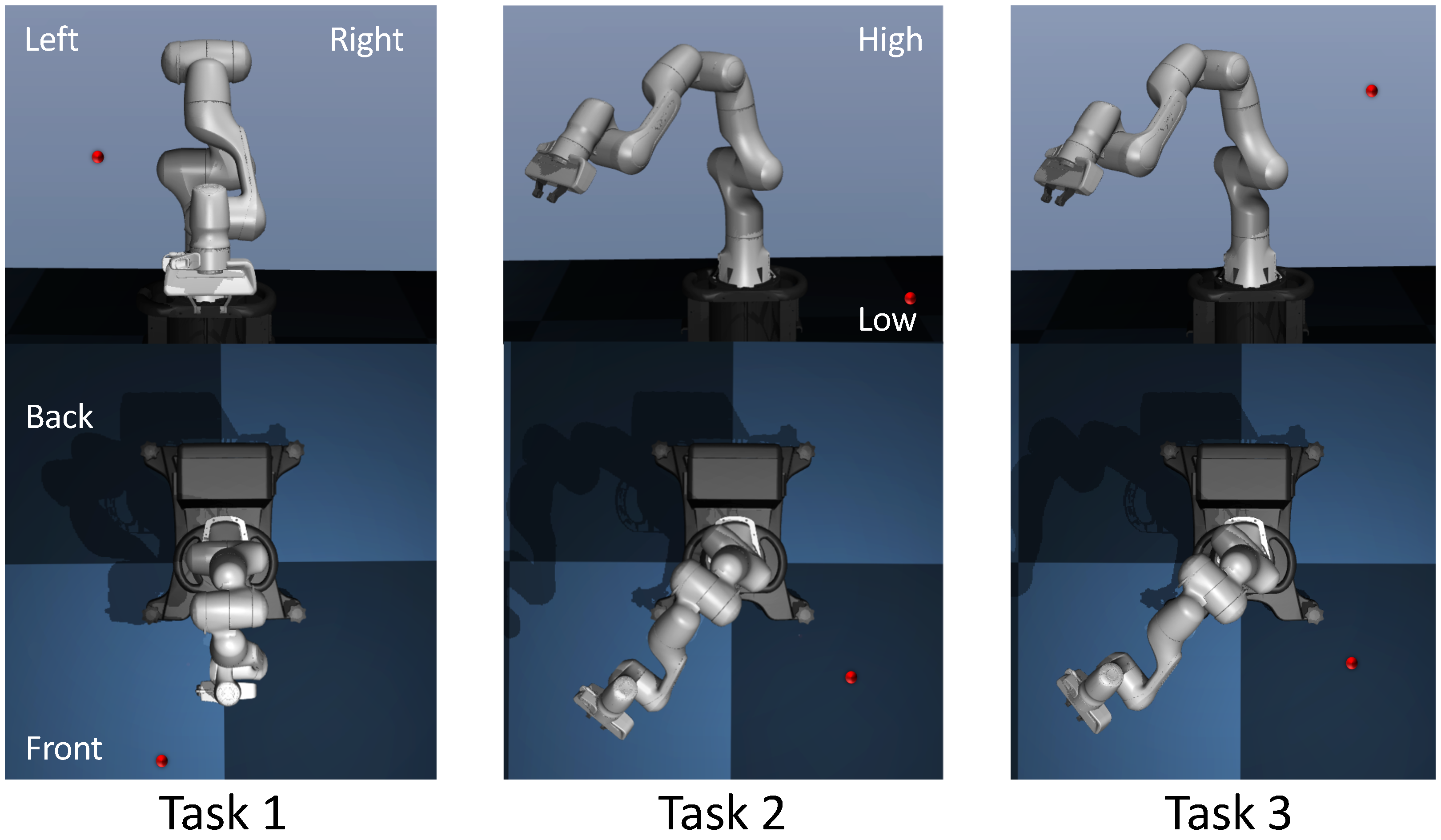
The resulting initial end-effector position, , and determined goal locations, , for Task 1, 2, and 3 are listed in Table 2. The value of differs between all tasks, and the values of and differ between Task 1 and Tasks 2–3, resulting different values between Task 1 and Tasks 2–3. The locations are listed in 3 dimensional coordinates, and the units for each location is in centimeters. The origin of the axis is placed at the center of the base of the robot arm.
In addition, the corresponding illustration is shown in Figure 2. In the robot environment, we define left and right, as the observer’s left and right, respectively, when facing the robot (see upper three images in Figure 2). We define front and back as the area in front and behind the robot, respectively, from the observer’s perspective. High and low refer to the upward and downward directions, respectively, from the observer’s perspective.
In Task 1, the initial end-effector position is low and directly in front of the robot, and the goal location is at about mid-height of the crouched robot arm, where is elevated above the robot base and the initial end-effector pose. We start with small variance for Task 1 to ensure reliable training such that Task 1 may serve not only as one of our experiments, but also as a baseline for comparison with Tasks 2–3. The robot links are connected end-to-end, so the small variance in initial joint angles leads to variance in the end-effector position close to 1 cm as seen in Table 1 and Table 2. In order to reach the goal location, ideally, sweeps from back to front of the robot, sweeps from right to left, and sweeps from low to high as shown in Figure 2, where represents dimension of the current coordinates, .
In Task 2, we lower the goal location and move it further away from the initial end-effector position. We change the initial angle of joints 1 and 4 to elevate the end-effector about 20 cm above the Task 1’s posture and rotated 45 degrees to the left as seen in Task 2 of Figure 2. We also increase the variance of each initial joint angle to rad. As the effect cascades through each of the joints, the variance of the end-effector became significant to the point that the variance for each dimension gets closer to 10 cm seen in Table 2. The increased variance of the initial position makes the task harder to solve, but it also makes the solution generalize to more initial joint configurations. The change in the elevation of the end-effector is significant since in Task 1 the end-effector was below the goal location, in Task 2 it is above the goal location.
4.3. RL Agents: ACKTR and PPO2
We test our controllers with RL agents ACKTR and PPO2 from OpenAI’s Stable Baselines [34]. We experiment with these two RL algorithms to validate if our results are consistent with RL agents. These two algorithms are adequate in our experiments to provide a good understanding of the effects of gravity compensation.
One way to reduce data correlation is to run multiple episodes simultaneously collecting multiple unique trajectories at once. In essence, the RL agent maintains a single policy that is shared by multiple RL workers which collect the trajectory data. Each RL worker applies the policy in its own episode or copy of the environment. Each of these RL workers accumulates trajectory data ( and after a set number of time steps the RL agent performs a policy update using the gradients computed from the trajectory data from all the RL workers. This method has not only been shown to reduce variance, but also has the added advantage of being parallelizable [38]. In our experiments we use four RL workers.
The reward function in all tasks for both RL agents is given by
In this reward function, and are the 3 dimensional coordinates of the current () and goal position (), respectively, and is the unit step function. This reward monotonically deceases with the distance of the end-effector from the goal position. The step function provides a linearly decreasing term that is zero for large distances. The hyperbolic tangent signal provides a small non-zero reward at large distances. More importantly, it provides a reward gradient that enables learning when the error is large.
The environment being solved is a task-space reaching task, where the agent must command the robot to move the end-effector of the robot arm to single specified location in 3D space and hold it there for the remainder of the episode. The environment returns a reward that increases as the agent moves the arm such that the end-effector approaches the goal location defined in 3D space.
This reaching environment terminates after 500 time-steps, far more than necessary to complete each task. We choose this high value to discover whether the RL algorithm stabilizes the goal state, and not just reaches it. We expect stabilization since the longer the arm stays at the goal state, the more rewards are earned. Controllers applied to this environment operate at 10 Hz while the actual simulation operates at 500 Hz. Therefore, each action is held constant for 50 time steps, which enables the state to change enough between updates to facilitate learning.
It should also be noted that for the 3 tasks we defined, the observations for the agent were scaled and shifted so that the values in each dimension were within the interval [0, 1]. The actions were also scaled and shifted so that the values for each dimension were within the interval [−1, 1]. This type of normalization was done to conform to recommendations made by the RL repository we used [34].
5. Results
We evaluate the results of running each RL agent with gravity compensated and uncompensated controller in each task described in Section 4. Our results show that gravity compensation tends to lead to faster training, but this advantage depends on the goal location and the initial pose of the robot. We discuss the behavior of the system when operating with a trained agent.
5.1. Hyperparameter Selection in RL Agents
To obtain optimal controllers used by the RL agent, we used a grid search approach. Grid search, Bayesian optimization [39], evolutionary optimization [40], and gradient optimization [41] are popularly considered ways to tune hyperparameters. However, gradient optimization is not readily extensible to the RL agents, and both Bayesian and evolutionary optimization algorithms depend on randomization and therefore can have varying performance over multiple runs. Our grid search over a discrete set of hyperparameter values included 192 permutations of unique hyperparameter selections for ACKTR and 128 permutations for PPO2. Ten training sessions were run for each permutation of hyperparameters. Each ACKTR training session was run for time steps while PPO2 was run for time steps. The specific number of time steps chosen for each run of ACKTR and PPO2 corresponded to the smallest number of time steps necessary to accumulate near the maximum reward using the best hyperparameter selection found in our initial experiments. One time step refers to one step taken in the environment.
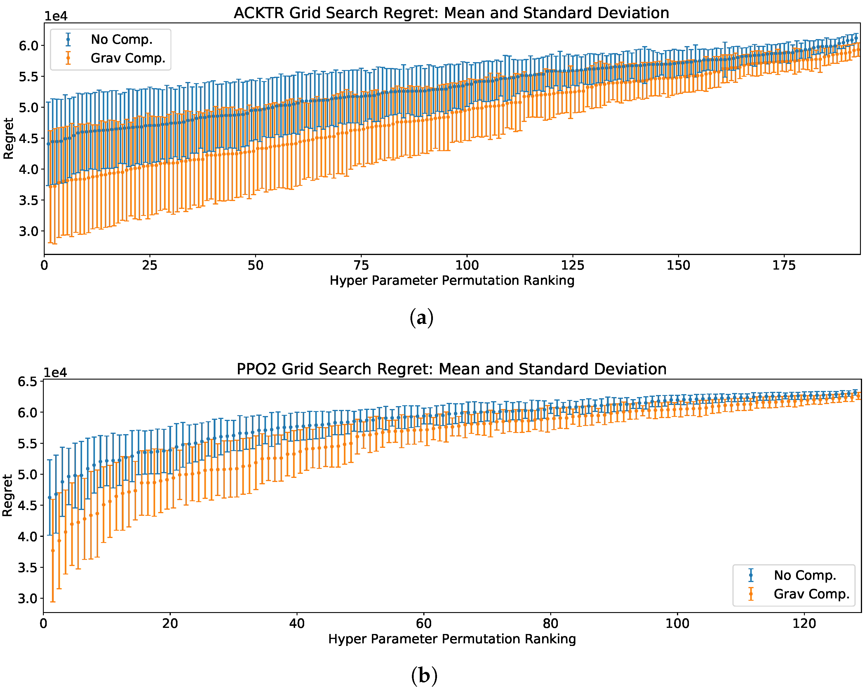
We measured the effectiveness of each training session by computing the cumulative regret over the entire training session. We compute regret by subtracting the episodic reward from the optimal episodic reward. Using this definition of regret, it can be seen that maximizing the cumulative reward is analogous to minimize the regret. We approximate the optimal episodic reward by assuming it is possible to collect the maximum reward for every time step of the episode. This is an upper bound since the inertia of the system does not allow it to move to the goal position for the first several time steps.
The plotted mean and standard deviation of the cumulative regret for both RL agents paired with both compensated and uncompensated systems with Task 1 are shown in Figure 3.
The detailed results are included in Supplementary Tables S1–S4. It is seen that over the hyperparameter selections compared, rank for rank, the gravity compensated system experiences less cumulative regret than the uncompensated system. This suggests that the region of explored hyperparameter space that results in fast training for both agents is larger for the gravity compensated system than the uncompensated system.
5.2. Performances on Task 1, 2, and 3
Once the hyperparameter set is selected for ACKTR and PPO2 agents with gravity compensated and uncompensated systems, ACKTR and PPO2 agents were trained for both gravity compensated and uncompensated systems in Task 1, 2, and 3 described in Section 4. The RL agents were evaluated by plotting the learning curves during training. The learning curves consist of the episodic reward received by a policy plotted against the number of policy update steps used to train that policy. These learning curves indicate how quickly the agent can learn a policy that achieves high episodic rewards.
Since each training session is stochastic, we evaluated the learning curves of each algorithm from 100 training sessions. We also observed how well each algorithm performs the task by observing both the actions taken and the states visited when the system is operating under the control of a trained RL agent. We begin with presenting the results of the 100 training sessions for each RL agent paired with each controller. Note that each training session starts from a different random initialization.
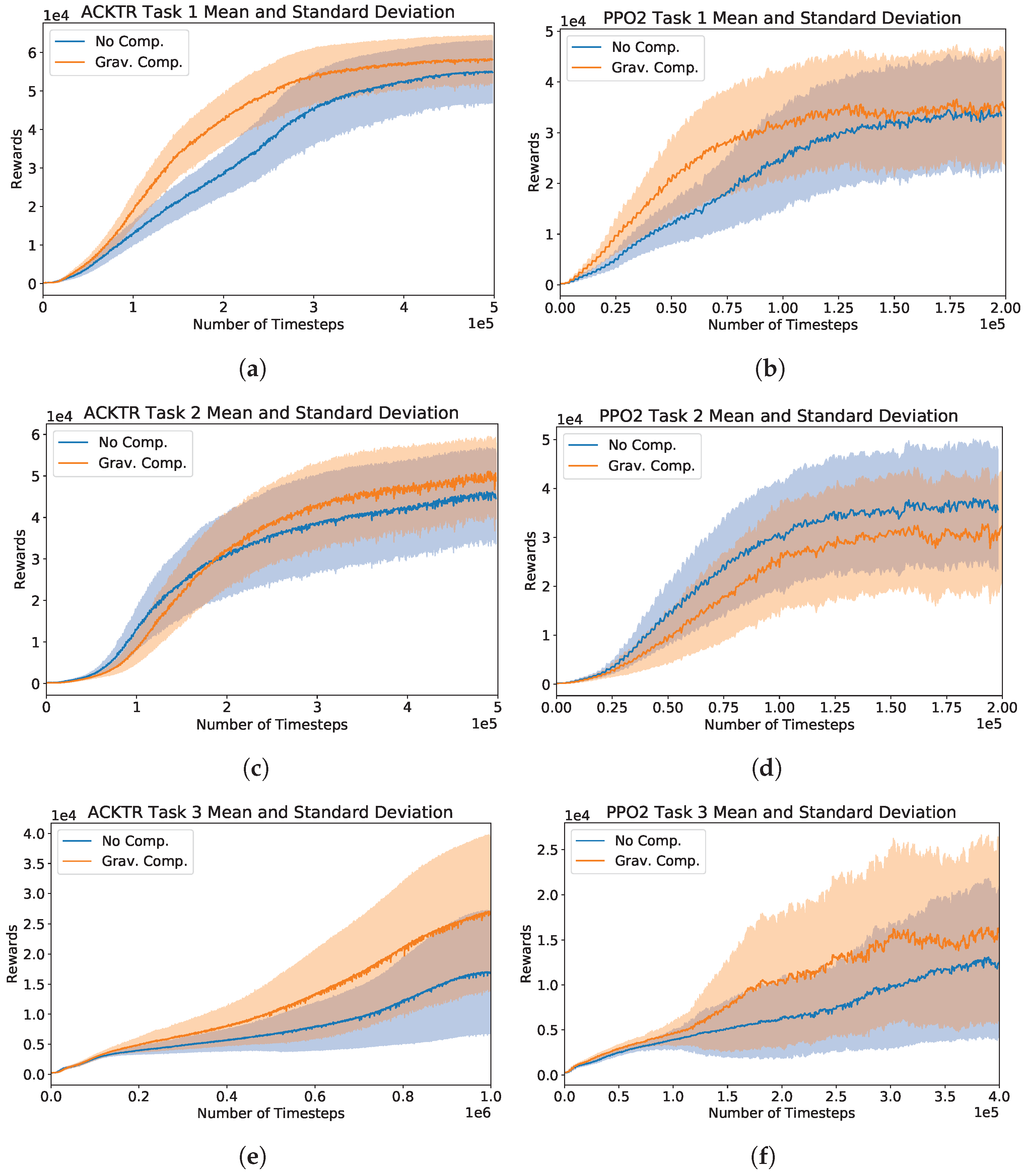
Figure 4 shows our results. Plots in the left column show learning curves from ACKTR, and plots in the right column are learning curves from PPO2. Plots in each row correspond to different task type. Each plot shows the mean and standard deviation of the episodic rewards as a function of the number of time steps with gravity compensated (orange lines) and uncompensated systems (blue lines). ACKTR and PPO2 agent was trained for and time steps for Task 1 and 2 and and time steps for Task 3, respectively. The number of time steps was chosen based on the time steps where learning curves plateau.
We can see that with the ACKTR agent, the gravity compensated system (orange lines) trains faster than the uncompensated system (blue lines) in all tasks (Figure 4a,c,e), and the gravity compensated system has a lower variance in Task 1 and 2 (Figure 4a,c). These conditions indicate reliable and productive training. In the case of PPO2 agent, the gravity compensated system trains faster than the system without compensation in Task 1 and 3 (Figure 4b,d).
In Task 1, while the mean reward for both systems with PPO2 is near after time steps, the trend is not upward like the ACKTR agent, and the variance is much greater. This may be because ACKTR employs a natural gradient method, which has better assurance for policy improvement, whereas PPO2 is a trust region method, which does not have a strong guarantee for policy improvement.
In Task 2, it is shown that for both systems, ACKTR does not learn Task 2 as quickly as Task 1. As noted in Table 2, the goal used in Task 2 is in the plane of the robot base whereas the goal in Task 1 is 0.4 meters above the plane of the robot base. We suspect that the uncompensated system is able to learn quicker in Task 2 due to the goal location being lower and more in the direction that gravity is pulling the system. In addition, we ascribe the higher variance in Task 2 compared to Task 1 to the increased variance in the robot’s initial position.
In Task 2, the learning curves from PPO2 are similar to the PPO2 results from Task 1 except that PPO2 with the uncompensated system trains faster that the compensated system. From this result, in addition to the reduced advantage of the compensated system with ACKTR agent in Task 2, we hypothesize that the elevation of the goal location affects how quickly the agents with the compensated and uncompensated systems are able to maximize the episodic rewards.
In Task 3, we explore this hypothesis further. We train the PPO2 agent with the same initialization of the robot pose as in Task 2, but the goal location is raised 0.5 meters (see Task 3 in Figure 2). Although both agents learn slower, the agents with the gravity compensated system train faster than with the uncompensated system (see Figure 4e,f). The training sessions that do not show improvement or very little improvement as the number of time steps increases, could be due to an unfavorable initialization of the policy or robot pose.
5.3. Agents’ Behavioral Evaluation
The agents’ behavior is captured by the states visited and the actions taken during 10 episodes. This type of analysis is critical in RL because it is possible that the RL agent learns to maximize reward in a way that is unexpected or unfavorable to our purposes. We selected agents by iterating over 100 training sessions and finding the first trained agent that was able to obtain more than episodic reward. It is acknowledged that different agents trained in the same experiment may exhibit different behavior, but we found the general behavior of agents operating on the same task to be very similar. Joint angle and agent action distributions in each case can be seen under supplementary materials (Figures S1–S20).
For Task 1, we found that the optimal policy tended to choose actions at or near the upper or lower limits for five of the joint torques while the remaining two joint torques would toggle between the extreme values or be distributed over some range of values. This resulted in joint angles that were near their upper or lower limits. The goal location in Task 1 is such that it is possible to reach with most joints held at or near their limits.
For Task 2, the actions selected were similar to the ones in Task 1, but they resulted in 1 or 2 joint angles that were not near either limit. It is likely that the location of the goal for Task 2 requires at least 1 joint angle to be some value between the limits. This requirement in addition to the high variance in the initial joint pose for this task may have caused slower training for Task 2 relative to Task 1.
In Task 3, at the agent’s selected actions where at most 4 of the values were at their limits and 3 or 4 of the other joint torques toggled between the extrema or were distributed over some region between the limits. We expect that this is the leading factor in the significantly slower training noted between Task 3 and Tasks 1 and 2. The distribution of joint angles for Task 3 has 3 joint angles that are well between the joint angle limits. We expect that the goal location for Task 3 required that more of the joints angles to be between their upper and lower limits.
The policies found by the agents in Tasks 1–3 may not be considered optimal when considering the ware on the system or the energy expended to accomplish the task; however, none of these considerations were encoded in the reward function. The reward function we use only incentivizes quickly reaching the goal location. Given the simplicity of the actions taken (relative to 7 torques chosen well between the action limits), it seems reasonable for the RL agents to converge to such a solution. If more of the seven action dimensions may be held constant the agent has effectively reduced the dimension of the problem.
We attempted to penalize the reward when the agent caused the joint angles to reach their limits and in a separate experiment we increased the reward when the system was near the center of the joint angle ranges; however, we found that both of these approaches lead to slower and less stable learning. We suspect that it is much more difficult for the RL agent to determine the optimal action in a high dimensional action space with multiple objectives encoded into a one dimensional reward function. There have been attempts to optimize multiple objectives. The authors of [18] do this by training the agent with a single objective encoded in the reward function (like minimizing the distance to the goal position) and then training the same agent with an additional objective encoded in the reward function (like minimizing expended energy). There are also other methods like multi-objective RL [42]. We do not address either of these methods in our experiments.
6. Discussion
The learning curves (Figure 4) showed how fast the agents were able to learn in comparison to the integration of the two popularly used RL agents with gravity compensated and uncompensated controller. The learning speed is especially critical in online implementations. It is notable that brain machine interface (BMI) is one considerable online implementation that can benefit from using our proposed method. A BMI architecture based on reinforcement learning has been introduced, called RLBMI [15]. In RLBMI, there are two intelligent systems: the BMI decoder in the agent to manipulate an external device, and the user in the environment. The two intelligent systems learn co-adaptively based on the closed-loop feedback. The agent updates the state of the environment, namely, a robotic arm’s location, based on the user’s neural activity and the received rewards. In this paradigm, the state representation is considered as the user’s neural activity, which is different from conventional RL approaches; that is, in a robotic arm control by using RL, the robotic arm’s kinematics are considered as the states, as we implemented in this study. Through iterations, both the BMI user and the neural decoder learn how to accomplish their mutual goal, by earning rewards based on their joint behavior. The BMI decoder learns a control strategy based on the user’s neural state and performs actions in goal directed tasks that update the state of the external device in the environment. In addition, the user learns the task based on the state of the external device. Note that both systems act symbiotically by sharing the external device to complete the task, and this bidirectional interaction allows for continuous synergistic adaptation between the BMI decoder and the user, even in a changing environment. In addition, successful applications of RLBMI can be found in several studies [16,43,44,45,46], where new neural decoders are introduced and validated in BMIs.
7. Conclusions
We introduced an approach to combine RL and control theory by adding terms used in a classical controller to the RL output. We provided a comparison of two controllers, learned using two different RL algorithms and showed that a good choice of controllers can reduce the training required by the RL agents without the need of a complete system model. Specifically, we trained ACKTR and PPO2 agents coupled with gravity compensated and uncompensated torque controls to complete 3 different reaching tasks with a simulated seven-degree-of-freedom robotic arm. We showed that the gravity compensated torque control leads to faster training when the goal location is elevated. Our results suggested that the uncompensated system performs worse with an elevated goal location since gravity adds a downward bias. This could cause the system to explore in regions of the state space that are not near the elevated goal while the compensated system has no bias and can explore all regions of the state space more uniformly. It is also observed that the PPO2 agent trains faster with the uncompensated torque control when the goal location is low, which may be due to the gravity bias pulling the system in the direction of the goal.
Although choice of RL algorithm is not the focus of our experiments, it should be noted that this choice significantly impacts training. We have chosen two sophisticated algorithms and have found that PPO2 can train five times faster than ACKTR, but that PPO2 has significantly higher variance between training sessions. We chose to experiment with ACKTR due to its stability, since it is a trust region method, and provides assurance for policy improvement, by using natural gradient. We chose PPO2 due to its promising performance in other robotics tasks [28] and because it does not use a natural gradient which yields more diversity in the RL algorithms we used. To expand our understanding of the effect of gravity compensated torque control, future research could include using additional RL algorithms to see if our results with ACKTR and PPO2 can generalize to more algorithms. It would also be instructive to add additional tasks such as reaching with a randomized goal location or a uniformly randomized initial position. These tasks could shed further light on how gravity compensation effects training with arbitrary goal locations. Uniformly randomizing the initial position would assist in understanding any effects gravity compensation has in training when the initial pose is arbitrary.
Supplementary Materials
The following are available online at https://www.mdpi.com/2218-6581/10/1/46/s1. The supplementary materials present the grid search results over hyperparameter permutations for the gravity compensated and uncompensated system with ACKTR (Tables S1 and S2) and PPO2 (Tables S3 and S4). In addition, supporting to Section 5.3, figures to depict joint angle and agent action distributions at each experimental case are presented (Figures S1–S20).
Author Contributions
Conceptualization, J.F., J.B. and H.A.P.; methodology, J.B. and H.A.P.; software, J.F.; validation, J.F.; data creation, J.F.; writing—original draft preparation, J.F., J.B., and H.A.P.; writing—review and editing, J.B., and H.A.P. All authors have read and agreed to the published version of the manuscript.
Funding
This research was funded by Department of Electrical and Computer Engineering at the University of Kentucky.
Institutional Review Board Statement
Not applicable.
Informed Consent Statement
Not applicable.
Data Availability Statement
The data, codes, and their corresponding results for this research work are available in the following GitHub link: https://github.com/jfugal3/ThesisPython.
Acknowledgments
Authors thank to anonymous reviewers who gave useful comments and to Department of Electrical and Computer Engineering at the University of Kentucky that provided financial support.
Conflicts of Interest
The authors declare no conflict of interest. The funders had no role in the design of the study; in the collection, analyses, or interpretation of data; in the writing of the manuscript, or in the decision to publish the results.
References
- Rottmann, A.; Mozos, O.M.; Stachniss, C.; Burgard, W. Semantic Place Classification of Indoor Environments with Mobile Robots Using Boosting. In Proceedings of the 20th National Conference on Artificial Intelligence, AAAI’05, Pittsburgh, PA, USA, 9–13 July 2005; Volume 3, pp. 1306–1311. [Google Scholar]
- Spong, M.W.; Hutchinson, S.; Vidyasagar, M. Robot Modeling and Control; Wiley and Sons: New York, NY, USA, 2006. [Google Scholar]
- Safiotti, A. Fuzzy logic in autonomous robotics: Behavior coordination. In Proceedings of the 6th International Fuzzy Systems Conference, Barcelona, Spain, 5 July 1997; Volume 1, pp. 573–578. [Google Scholar] [CrossRef]
- Chen, C.H.; Wang, C.C.; Wang, Y.T.; Wang, P.T. Fuzzy Logic Controller Design for Intelligent Robots. Math. Probl. Eng. 2017. [Google Scholar] [CrossRef]
- Antonelli, G.; Chiaverini, S.; Sarkar, N.; West, M. Adaptive control of an autonomous underwater vehicle: Experimental results on ODIN. In Proceedings of the 1999 IEEE International Symposium on Computational Intelligence in Robotics and Automation, CIRA’99 (Cat. No.99EX375), Monterey, CA, USA, 8–9 November 1999; pp. 64–69. [Google Scholar] [CrossRef]
- Wei, B. A Tutorial on Robust Control, Adaptive Control and Robust Adaptive Control—Application to Robotic Manipulators. Inventions 2019, 4, 49. [Google Scholar] [CrossRef] [Green Version]
- Bicho, E.; Schöner, G. The dynamic approach to autonomous robotics demonstrated on a low-level vehicle platform. Robot. Auton. Syst. 1997, 21, 23–35. [Google Scholar] [CrossRef] [Green Version]
- Schöner, G.; Dose, M.; Engels, C. Dynamics of behavior: Theory and applications for autonomous robot architectures. Robot. Auton. Syst. 1995, 16, 213–245. [Google Scholar] [CrossRef]
- Fu, J.; Luo, K.; Levine, S. Learning Robust Rewards with Adversarial Inverse Reinforcement Learning. arXiv 2018, arXiv:1710.11248. [Google Scholar]
- Bogert, K.; Doshi, P. Multi-robot inverse reinforcement learning under occlusion with estimation of state transitions. Artif. Intell. 2018, 263, 46–73. [Google Scholar] [CrossRef]
- Kober, J.; Bagnell, J.A.; Peters, J. Reinforcement learning in robotics: A survey. Int. J. Robot. Res. 2013, 32, 1238–1274. [Google Scholar] [CrossRef] [Green Version]
- Gu, S.; Holly, E.; Lillicrap, T.; Levine, S. Deep Reinforcement Learning for Robotic Manipulation with Asynchronous Off-Policy Updates. In Proceedings of the IEEE International Conference on Robotics and Automation (ICRA), Singapore, 29 May–3 June 2017; pp. 3389–3396. [Google Scholar]
- Levine, S.; Finn, C.; Darrell, T.; Abbeel, P. End-to-End Training of Deep Visuomotor Policies. arXiv 2015, arXiv:1504.00702. [Google Scholar]
- Li, W.; Todorov, E. Iterative Linear Quadratic Regulator Design For Nonlinear Biological Movement Systems. In Proceedings of the First International Conference on Informatics in Control, Automation and Robotics, Setúbal, Portugal, 25–28 August 2004. [Google Scholar] [CrossRef] [Green Version]
- DiGiovanna, J.; Mahmoudi, B.; Fortes, J.; Principe, J.C.; Sanchez, J.C. Coadaptive Brain–Machine Interface via Reinforcement Learning. IEEE Trans. Biomed. Eng. 2009, 56, 54–64. [Google Scholar] [CrossRef]
- Bae, J.; Sanchez Giraldo, L.G.; Pohlmeyer, E.A.; Francis, J.T.; Sanchez, J.C.; Príncipe, J.C. Kernel Temporal Differences for Neural Decoding. Intell. Neurosci. 2015, 2015. [Google Scholar] [CrossRef] [Green Version]
- Abbeel, P.; Coates, A.; Quigley, M.; Ng, A.Y. An application of reinforcement learning to aerobatic helicopter flight. In Proceedings of the Advances in Neural Information Processing Systems, Vancouver, BC, Canada, 4–7 December 2007; pp. 1–8. [Google Scholar]
- Martín-Martín, R.; Lee, M.A.; Gardner, R.; Savarese, S.; Bohg, J.; Garg, A. Variable Impedance Control in End-Effector Space: An Action Space for Reinforcement Learning in Contact-Rich Tasks. arXiv 2019, arXiv:1906.08880. [Google Scholar]
- Johannink, T.; Bahl, S.; Nair, A.; Luo, J.; Kumar, A.; Loskyll, M.; Ojea, J.A.; Solowjow, E.; Levine, S. Residual Reinforcement Learning for Robot Control. In Proceedings of the 2019 International Conference on Robotics and Automation (ICRA), Montreal, QC, Canada, 20–24 May 2019. [Google Scholar] [CrossRef] [Green Version]
- Arakelian, V. Gravity compensation in robotics. Adv. Robot. 2015, 30, 1–18. [Google Scholar] [CrossRef]
- Ernesto, H.; Pedro, J.O. Reinforcement learning in robotics: A survey. Math. Probl. Eng. 2015. [Google Scholar] [CrossRef] [Green Version]
- Yu, C.; Li, Z.; Liu, H. Research on Gravity Compensation of Robot Arm Based on Model Learning. In Proceedings of the 2019 IEEE/ASME International Conference on Advanced Intelligent Mechatronics (AIM), Hong Kong, China, 8–12 July 2019; pp. 635–641. [Google Scholar] [CrossRef]
- Montalvo, W.; Escobar-Naranjo, J.; Garcia, C.A.; Garcia, M.V. Low-Cost Automation for Gravity Compensation of Robotic Arm. Appl. Sci. 2020, 10, 3823. [Google Scholar] [CrossRef]
- Alothman, Y.; Gu, D. Quadrotor transporting cable-suspended load using iterative linear quadratic regulator (ilqr) optimal control. In Proceedings of the 2016 8th Computer Science and Electronic Engineering (CEEC), Colchester, UK, 28–30 September 2016; pp. 168–173. [Google Scholar]
- Puterman, M.L. Markov Decision Processes: Discrete Stochastic Dynamic Programming, 1st ed.; John Wiley & Sons, Inc.: Hoboken, NJ, USA, 1994. [Google Scholar]
- Sutton, R.S.; Barto, A.G. Reinforcement Learning: An Introduction, 2nd ed.; Adaptive Computation and Machine Learning Series; The MIT Press: Cambridge, MA, USA, 2018. [Google Scholar]
- Wu, Y.; Mansimov, E.; Liao, S.; Grosse, R.B.; Ba, J. Scalable trust-region method for deep reinforcement learning using Kronecker-factored approximation. arXiv 2017, arXiv:1708.05144. [Google Scholar]
- Schulman, J.; Wolski, F.; Dhariwal, P.; Radford, A.; Klimov, O. Proximal Policy Optimization Algorithms. arXiv 2017, arXiv:1707.06347. [Google Scholar]
- Henderson, P.; Islam, R.; Bachman, P.; Pineau, J.; Precup, D.; Meger, D. Deep Reinforcement Learning that Matters. arXiv 2017, arXiv:1709.06560. [Google Scholar]
- Aumjaud, P.; McAuliffe, D.; Rodriguez Lera, F.J.; Cardiff, P. Reinforcement Learning Experiments and Benchmark for Solving Robotic Reaching Tasks. In Proceedings of the 21st International Workshop of Physical Agents (WAF 2020), Madrid, Spain, 19–20 November 2020. [Google Scholar] [CrossRef]
- Amari, S.I. Natural Gradient Works Efficiently in Learning. Neural Comput. 1998, 10, 251–276. [Google Scholar] [CrossRef]
- Kakade, S.M. A Natural Policy Gradient. In Proceedings of the 14th International Conference on Neural Information Processing Systems: Natural and Synthetic; MIT Press: Cambridge, MA, USA, 2001; pp. 1531–1538. [Google Scholar]
- Schulman, J.; Levine, S.; Moritz, P.; Jordan, M.I.; Abbeel, P. Trust Region Policy Optimization. arXiv 2017, arXiv:1502.05477. [Google Scholar]
- Hill, A.; Raffin, A.; Ernestus, M.; Gleave, A.; Kanervisto, A.; Traore, R.; Dhariwal, P.; Hesse, C.; Klimov, O.; Nichol, A.; et al. Stable Baselines. 2018. Available online: https://github.com/hill-a/stable-baselines (accessed on 1 June 2019).
- Grosse, R.; Martens, J. A Kronecker-factored approximate Fisher matrix for convolution layers. arXiv 2016, arXiv:1602.01407. [Google Scholar]
- Fan, L.; Zhu, Y.; Zhu, J.; Liu, Z.; Zeng, O.; Gupta, A.; Creus-Costa, J.; Savarese, S.; Fei-Fei, L. SURREAL: Open-Source Reinforcement Learning Framework and Robot Manipulation Benchmark. In Proceedings of the Conference on Robot Learning, Zürich, Switzerland, 29–31 October 2018. [Google Scholar]
- Todorov, E.; Erez, T.; Tassa, Y. MuJoCo: A physics engine for model-based control. In Proceedings of the 2012 IEEE/RSJ International Conference on Intelligent Robots and Systems, Vilamoura-Algarve, Portugal, 7–12 October 2012; pp. 5026–5033. [Google Scholar] [CrossRef]
- Babaeizadeh, M.; Frosio, I.; Tyree, S.; Clemons, J.; Kautz, J. GA3C: GPU-based A3C for Deep Reinforcement Learning. arXiv 2016, arXiv:1611.06256. [Google Scholar]
- Falkner, S.; Klein, A.; Hutter, F. BOHB: Robust and Efficient Hyperparameter Optimization at Scale. arXiv 2018, arXiv:1807.01774. [Google Scholar]
- Li, L.; Jamieson, K.; DeSalvo, G.; Rostamizadeh, A.; Talwalkar, A. Hyperband: A Novel Bandit-Based Approach to Hyperparameter Optimization. J. Mach. Learn. Res. 2017, 18, 6765–6816. [Google Scholar]
- Paul, S.; Kurin, V.; Whiteson, S. Fast Efficient Hyperparameter Tuning for Policy Gradients. arXiv 2019, arXiv:1902.06583. [Google Scholar]
- Liu, C.; Xu, X.; Hu, D. Multiobjective Reinforcement Learning: A Comprehensive Overview. IEEE Trans. Syst. Man Cybern. Syst. 2015, 45, 385–398. [Google Scholar]
- Pohlmeyer, E.A.; Mahmoudi, B.; Geng, S.; Prins, N.W.; Sanchez, J.C. Using Reinforcement Learning to Provide Stable Brain-Machine Interface Control Despite Neural Input Reorganization. PLoS ONE 2014, 9, e87253. [Google Scholar] [CrossRef] [Green Version]
- An, J.; Yadav, T.; Ahmadi, M.B.; Tarigoppula, V.S.A.; Francis, J.T. Near Perfect Neural Critic from Motor Cortical Activity Toward an Autonomously Updating Brain Machine Interface. In Proceedings of the 2018 40th Annual International Conference of the IEEE Engineering in Medicine and Biology Society (EMBC), Honolulu, HI, USA, 17–21 July 2018; pp. 73–76. [Google Scholar] [CrossRef]
- Shaikh, S.; So, R.; Sibindi, T.; Libedinsky, C.; Basu, A. Towards Autonomous Intra-Cortical Brain Machine Interfaces: Applying Bandit Algorithms for Online Reinforcement Learning. In Proceedings of the 2020 IEEE International Symposium on Circuits and Systems (ISCAS), Seville, Spain, 10–21 October 2020; pp. 1–5. [Google Scholar] [CrossRef]
- Shen, X.; Zhang, X.; Huang, Y.; Chen, S.; Wang, Y. Task Learning Over Multi-Day Recording via Internally Rewarded Reinforcement Learning Based Brain Machine Interfaces. IEEE Trans. Neural Syst. Rehabil. Eng. 2020, 28, 3089–3099. [Google Scholar] [CrossRef]
Figure 1.
Framework for Residual Reinforcment Learning. A controller’s output is combined with a policy learned by a reinforcement learning agent to control a robot. The environment for the RL agent is the closed-loop robot control system.
Figure 1.
Framework for Residual Reinforcment Learning. A controller’s output is combined with a policy learned by a reinforcement learning agent to control a robot. The environment for the RL agent is the closed-loop robot control system.

Figure 2.
Visualization of initial robot poses and goal locations for Tasks 1–3. In these images the goal location is indicated by the red dot.
Figure 2.
Visualization of initial robot poses and goal locations for Tasks 1–3. In these images the goal location is indicated by the red dot.

Figure 3.
Grid-search results for the ACKTR and PPO2 reinforcement learning agents. The mean and the standard deviation of the cumulative regret in the 10 training sessions corresponding to each hyperparameter permutation are shown. The center point of each bar being the mean cumulative regret while the total length of the bar indicates the standard deviation. The system with gravity compensation is slightly shifted to the right to enhance visibility. The results for each system are displayed in ascending order of the mean cumulative regret. (a) Gravity compensation leads to lower regret for all hyperparameters permutations when training using the ACKTR algorithm. (b) Gravity compensation leads to lower regret for all hyperparameters permutations when training using the PPO2 algorithm.

Figure 4.
Training session learning curves of ACKTR and PPO2 RL agents on Tasks 1–3. The solid curve is the mean episode reward for the network during training, and the shaded region indicates the standard deviation. (a) In Task 1, ACKTR with gravity compensation achieves higher rewards than ACKTR without gravity compensation, and learns faster. (b) In Task 1, PPO2 with gravity compensation achieves similar rewards to PPO2 without gravity compensation. Gravity compensation appears to enable faster learning. (c) In Task 2, ACKTR with gravity compensation achieves higher rewards than ACKTR without gravity compensation, although the rewards are lower in the initial period of training. (d) In Task 2, PPO2 with gravity compensation achieves lower rewards than PPO2 without gravity compensation, and also learns slower. (e) In Task 3, ACKTR with gravity compensation achieves significantly higher rewards than ACKTR without gravity compensation, and also learns faster. (f) In Task 3, PPO2 with gravity compensation achieves higher rewards than PPO2 without gravity compensation, and also learns faster.


Table 1.
Mean and variance of the initial joint configurations for Task 1–3.
| Task 1 | (0, , 0, , 0, , ) | 0.0004 |
| Task 2–3 | (, , 0, , 0, , ) | 0.0025 |
Table 2.
The initial end-effector position and goal location for Task 1–3.
| Task 1 | (44.48 ± , 0.0 ± , 10.81 ± ) | (60, −20, 40) |
| Task 2 | (43.70 ± , −43.64 ± , 31.78 ± ) | (40, 40, 0) |
| Task 3 | (43.70 ± , −43.64 ± , 31.78 ± ) | (30, 30, 50) |
Publisher’s Note: MDPI stays neutral with regard to jurisdictional claims in published maps and institutional affiliations. |
© 2021 by the authors. Licensee MDPI, Basel, Switzerland. This article is an open access article distributed under the terms and conditions of the Creative Commons Attribution (CC BY) license (http://creativecommons.org/licenses/by/4.0/).
Share and Cite
MDPI and ACS Style
Fugal, J.; Bae, J.; Poonawala, H.A. On the Impact of Gravity Compensation on Reinforcement Learning in Goal-Reaching Tasks for Robotic Manipulators. Robotics 2021, 10, 46. https://doi.org/10.3390/robotics10010046
AMA Style
Fugal J, Bae J, Poonawala HA. On the Impact of Gravity Compensation on Reinforcement Learning in Goal-Reaching Tasks for Robotic Manipulators. Robotics. 2021; 10(1):46. https://doi.org/10.3390/robotics10010046
Chicago/Turabian StyleFugal, Jonathan, Jihye Bae, and Hasan A. Poonawala. 2021. "On the Impact of Gravity Compensation on Reinforcement Learning in Goal-Reaching Tasks for Robotic Manipulators" Robotics 10, no. 1: 46. https://doi.org/10.3390/robotics10010046
Note that from the first issue of 2016, this journal uses article numbers instead of page numbers. See further details here.