
Renormalizing Open Quantum Field Theories


1
Department of Theoretical Physics, University of Debrecen, P.O. Box 5, H-4010 Debrecen, Hungary
2
Physics and Engineering Department CNRS-IPHC, Strasbourg University, 23 Rue du Loess, CEDEX 2, 67037 Strasbourg, France
*
Author to whom correspondence should be addressed.
†
These authors contributed equally to this work.
Universe 2022, 8(2), 127; https://doi.org/10.3390/universe8020127
Submission received: 20 December 2021
/
Revised: 30 January 2022
/
Accepted: 14 February 2022
/
Published: 16 February 2022
(This article belongs to the Special Issue Quantum Field Theory of Open Systems)
Abstract
:The functional renormalization group flow of a scalar field theory with quartic couplings and a sharp spatial momentum cutoff is presented in four-dimensional Minkowski space-time for the bare action by retaining the entanglement of the IR and the UV particle modes. It is argued that the open interaction channels have to be taken into account in quantum field theory defined by the help of a cutoff, and a non-perturbative UV-IR entanglement is found in closed or almost closed models.
1. Introduction
One of the most important lessons of contemporary physics is that the observed phenomena depend qualitatively and quantitatively on the scales of observation. Hence rather than looking for a “World Equation” or “Theory Of Everything” one looks for effective theories, valid only in some scale window. We know several such theories, starting with the Standard Model of Particle Physics and ending with the Standard Model of Cosmology, and the challenge is to understand the way these models follow each other on their renormalized trajectory as the resolution of the observations is changed. The goal of this work is to orient the attention to an important feature of the effective theories, namely that they deal with open dynamics. However, this point is actually obvious, since the unobserved degrees of freedom represent an environment for the observed system the systematic addressing of the problem has been lacking. We choose the simplest non-trivial model for this purpose, describing a scalar field in 3 + 1 dimensions.
There is another reason to consider open theories. In the first phase of the history of quantum field theory, attention was turned towards renormalizable models by the help of renormalized perturbation expansion. However, the need to go beyond this approximation scheme introduced the cutoff theories, which are defined by a large but finite UV cutoff back into the foreground of the interest. The cutoff theories describe open dynamics, as well, since the degrees of freedom beyond the cutoff serve as an environment. One can go a bit further an state that the inherent UV divergences of quantum field theory simply exclude a truly closed quantum dynamics by rendering the cutoff necessary. One might object that an environment consisting of very energetic particle modes should not modify the low energy physics in an important manner. However the question is more involved and a detailed knowledge of the scaling laws are needed to understand the role of the open channels at high energy in the physics at low energy.
Our main results, obtained for the four-dimensional real scalar theory, are as follows: (i) The change of the cutoff towards either the IR or the UV direction renders the dynamics open, in other words, closed theories are inconsistent according to the renormalization group method. This is demonstrated explicitly in Section 3. (ii) There are open interaction vertices representing open interactions which are relevant and leave a trace on the physical quantities for arbitrarily high cutoff scale. (iii) The theory with sufficiently long lived quasi particles displays non-perturbative IR scaling and strong UV-IR entanglement, making the comparison of the quantum and the classical dynamics more difficult. Therefore quantum field theories should be used by allowing a mixed vacuum state. The most promising method to deal with open systems is the Closed Time Path (CTP) scheme (or Schwinger-Keldysh formalism) hence the renormalization of effective quantum field theories should be handled in that formalism.
The CTP formalism was first developed for the perturbation expansion in the Heisenberg representation [1,2,3]; however its subsequent use is increasingly in open quantum systems where the system-environment separation appears in different disguise in different physical problem. The decoherence [4,5], a necessary condition of the classical limit of quantum systems [6,7], can easily be grasped by establishing the additive probabilities of histories [8,9,10,11] in a macroscopic environment. The environment of an observed collective mode consists of the rest of the macroscopic system in non-equilibrium statistical physics [12,13]. The environment of a dissipative system remains unreachable [14,15]. The environment of driven nanophysical, solid state or optical devices is in the macroscopic domain [16]. The nano wires are imbedded into an environment of their leads [17]. A thermal reservoir can always be assumed as part of the environment, too. High energy physics applications stretch from thermal field theory [18] to astrophysics [19]. The path integral representation of quantum mechanics is particularly well suited to this formalism [20], the calculation we report below has been performed in the framework of the path integral representation of the CTP formalism, covered concisely in ref. [19]. The environment of a cutoff field theory is rather particular, it is provided by the UV modes which interact with the retained IR modes. Our goal is to discover the impact of the entanglement between the IR and the UV sectors on the IR dynamics.
The functional renormalization group method was already applied in the CTP formalism to follow the coarse graining [21,22,23], addressing a quantum dot [24], open electronic systems [25], the transport processes [26], the damping [27], the inflation [28], quantum cosmology [29] and critical dynamics [30,31,32,33]. Furthermore, it can describe the behavior of the Bose–Einstein condensate [34,35,36], the form of the spectral function [37,38], or real time dynamics of gauge theories [39]. The renormalization group scheme was extended to stochastic field theory [40], too. The need for bi-local terms in the action was argued in ref. [41]. The extension to the 2PI formalism has been used used to find non-thermal fixed points [42] and the renormalization group scheme can be transformed to trace the time dependence [43,44,45]. The one-loop renormalizability of the scalar model has been worked out on the one-loop level by the help of the more traditional multiplicative renormalization group method [46,47].
Before starting, it is worth distinguishing between a regulator and a cutoff of a field theory. The former renders the theory UV finite and the latter introduces a separation of the UV and the IR modes. A regulated theory, which is formulated in continuous space-time at arbitrarily large frequencies and wave vectors, can be called microscopic and a theory with a cutoff is necessarily effective. A cutoff of scale leaves the field modes with spatial three-momentum untouched in the IR and suppresses them completely in the UV for where and . The modes are neither IR nor UV. A cutoff with is called sharp and yields a well defined splitting of the degrees of freedoms into an IR and an UV class. A smooth cutoff with is only a regulator. In a regulated (UV finite) theory without cutoff the separation of the UV and the IR sector can be defined only qualitatively by introducing the UV regime for scales where the dynamics is strongly influenced by the regulator.
The choice of the width of a smooth cutoff, , represents a compromise. One the one hand, the width should be small to separate clearly the observed and the unobserved modes. On the other hand, the width should be large enough to avoid long range oscillations in the space-time. According to the traditional strategy, one uses the truncated gradient expansion as an ansatz for the action and such oscillations make this approximation scheme ill-defined even in Euclidean space-time where the dynamics is free of mass-shell singularities. However, the gradient expansion is a dead end street in constructing a systematic approximation to real time dynamics owing to Ostrogadsky’s instability [48,49] and should be replaced by the cluster expansion based on multi-local action functionals. By anticipating such a strategy for the future, we rely on the functional renormalization group method based on sharp cutoff with [50], used in the CTP formalism in the present work.
2. Open Quantum Systems
The lowering of the cutoff, the blocking, has to be performed by keeping track of the mixed state components generated by the elimination of the dynamical degrees of freedom. This can be achieved in the CTP formalism, outlined in this section.
2.1. Closed System
We start with the density matrix of a closed system,
where stands for the initial density matrix and denotes the time evolution operator of a closed dynamics. The path integral expression,
can be obtained by performing the usual slicing procedure in time for U and where denotes the doublet field, the integration is over the field configurations , the convolution with the initial density matrix at time is suppressed in the notation for simplicity and the action is given by , denoting the usual action of the closed theory.
The traditional formalism of quantum field theory dealing with transition amplitudes between pure states, , is called Single Time Path (STP) scheme. The reduplication of the degrees of freedom in (2) is to cope with the quantum fluctuations of the bra and the ket in (3). This is not necessary in closed dynamics for pure initial states, , where these fluctuations are independent and identical. The expression (2) of the density matrix belongs to the Open Time Path (OTP) scheme because the trajectories of the path integral are open, have different end points. The reduplication of the degrees of freedom is unavoidable in open systems where the non-factorizable density matrix of a mixed state describes correlated bra and ket fluctuations.
2.2. Open System
Let us now assume that we observe the dynamics of the field which is interacting with another field, , the full dynamics is closed and is described by the action . To assure the reader that the environment influences the observed system by the interactions taking place only during the observation time we assume that the system and its environment are not entangled at the initial time meaning that the initial density matrix factorizes as . We are interested in the reduced density matrix of the observed system,
given by the path integral expression, (2), and the effective action, . The influence functional describes the open interactions [20],
where the integration is over the field configurations and the convolution with the initial density matrix is suppressed represents the system-environment interactions.
It is advantageous to write the resulting effective action in the form
by separating the uncoupled and the coupled time axis contributions, . The independence of the bra and the ket fluctuations is reflected in the simple additive structure of the action and the single time axes contribution, , comprises the closed, conservative interactions. The coupling between the axis, , generates open classical forces, correlates the bra and ket fluctuations and renders the reduced density matrix mixed [51].
The physical content of the effective theory can be extracted from the generator functional for the connected Green functions,
where the system dynamics is extended by the introduction of the external source , coupled linearly to the field in the action, giving rise to the time evolution operator . This equation defines the CTP scheme because the path integral expression of the generator functional contains closed trajectory pairs owing to the trace over the Fock space. The shifts and is a symmetry of the dynamics due to the time translation invariance of the action. This symmetry, which is important in the STP formalism to keep the Green functions diagonal in the frequency space, is violated by the trace operation. To regain the symmetry and simplify the formalism, we perform the long evolution time limit, , , which renders the propagator of local excitations diagonal in the continuous frequency space. However this step is more involved as in the STP case [52]. In fact, this limit is assured in the latter case by Feynman’s prescription, the adiabatic suppression of the excitations for long time evolution. Rather than approaching slowly the vacuum, the final state is allowed to be chosen freely by the dynamics itself in the CTP formalism hence the dynamics is non-trivial at any finite .
Finally, a comment on the time reversal invariance. The limit and simplifies the time reversal transformation to , namely the CTP generator functional with an action and without any particular rule at the initial and the final time is time reversal invariant. The action of a closed dynamics is time reversal invariant in this limit. The influence functional (4) preserves this symmetry therefore open dynamics remains time reversal, as well. There is no contradiction with the presence of dissipative forces which may arise in an open dynamics since the time reversal, as defined above, reverses the direction of the time both for the system and for its environment. In particular, the coupling between the time axis generates terms in the (effective) equation of motion with broken time reversal symmetry [51].
2.3. Propagator
The limits and can easily be found for free quantum fields in the following manner. The dynamics defined by the translation invariant action
yields the generator functional
with the CTP propagator,
containing the Feynman propagator and its complex conjugate in the diagonal and the Wightman function in its off-diagonal blocks. First one calculates these functions in the operator formalism in the limit and for the vacuum as initial state,
for a scalar particle of mass m. Please note that the only source of the off-shell amplitudes in the propagator is the time ordering, the Wightman functions are on-shell and the Heaviside functions represent the vacuum initial condition. Next the kernel of the free action, the inverse propagator is found,
by direct inversion of (10) when the Dirac-delta distribution is represented by a regulated normalized Lorentzian peak.
The doublet fields are coupled only at the final time for finite . One would have thought that this coupling becomes unimportant in the limit . However, such a naive argument is misleading, since the suppression of the coupling between the doublets removes the trace in (6) for whatever large we use. According to (11), the limit indeed suppresses the coupling at and renders the dynamics translation invariant in time, but the two time axes remain coupled by an infinitesimal, time translation invariant operator, the off-diagonal elements on the right had side of (11). This coupling represents the difference between the CTP and the STP schemes and is non-local in time,
to assure that the elementary excitations above the vacuum, propagating with (10), correspond to positive energies.
2.4. Initial State
The initial state in (3) influences the effective action for the observed subsystem. We choose the perturbative vacuum as initial state in the limit and assume the usual adiabatic building up the true, interactig vacuum. This procedure can be summarized by stating that the excitations over the initial state can only have positive energy.
To assess the importance of the positivity of the excitation energies, let us consider the off-diagonal block of the propagator,
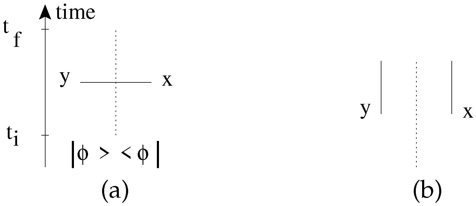
where the trace is obtained by summing over the stationary states of the full closed dynamics. The contributions come from excited bra and ke states, and , respectively. Hence this block of the propagator is non-vanishing only for positive energies states , c.f. Figure 1 and Equation (11). A similar argument applies to which is non-vanishing for negative energies. It is easy to see that this structure is inherited by the higher order Green function; in addition, is vanishing when the total energy flowing from the legs to is negative.
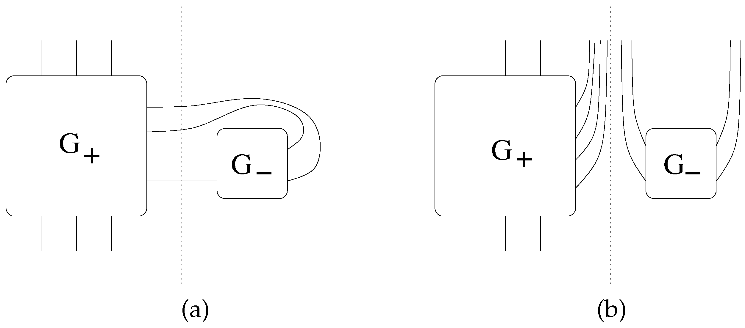
Such a restriction leads to a remarkable simplification of the interactive Green functions [51]. The CTP Feynman graphs can be grouped into three classes: the homogeneous graphs are where all external and internal lines belong to the same CTP copy. The external legs correspond to the same CTP copy but there are end points of the internal lines land at both copies in inhomogeneous graphs. Finally, the genuine CTP graphs have external legs attached to both copies. The homogeneous graphs are identical to the their STP counterparts and the genuine CTP graphs represent processes which generate excitations at the final time. The interesting question is whether the inhomogeneous graphs differ in STP and CTP. The answer to this question is negative if the excitations have positive energy, cf. Figure 2.
2.5. Open Interaction Vertices
The action of an open dynamics couples the field variables corresponding to the bra and the ket. We have seen that such a coupling must be non-local in time and the simplest classification of non-local action is the cluster expansion. The lowest order which incorporates the condition of positive energy excitations is the bilocal level,
The kernel of the first term is the inverse of the massless free propagator (11) and the conservative interaction is described by a local potential,
The open interactions are represented by a bilocal potential,
where . Though one could in principle extend the ansatz by allowing a non-trivial dependence in such a restriction is needed for the invariance with respect to the orthochronuos Lorentz group, the subgroup of the full Lorentz group which preserves the direction of the time. The symmetry with respect to time reversal of the open system dynamics is broken by the initial condition of the environment. The potentials are complex, , , the imaginary part is generated by the intermediate states of the Feynman diagrams according to the optical theorem and the time reversal invariance of the full closed dynamics requires . A closed theory is obtained by the choice , and vanishing higher orders, for .
We use below the truncation with ,
One has in principle and vertices but their evolution is of fourth order in the cluster expansion hence they are ignored in our second order truncation scheme. In the absence of energy conservation, the stability follows from the finiteness of the path integral which amounts to . Since we assume the triviality of the saddle point for the blocking the condition has to be imposed, too.
2.6. UV-IR Entanglement and Decoherence
A distinguished feature of an open quantum system is that the system-environment entanglement renders the system state mixed. A mixed state consists of several pure states, the eigenstates of the density matrix, corresponding to a probability which is given by the corresponding eigenvalue. It is crucial to note that different pure states do not enter into interference with each other in the expectation value of observables [53]. Such a restriction of the coherence is usually called decoherence [4,5], defined roughly as the suppression of the off-diagonal elements of the density matrix. Naturally, such a definition depends on the basis where the off-diagonal elements are taken. The decoherence is displayed below in the field diagonal basis by the help of the influence functional [20].
It is enlightening to employ the parameterization , by interpreting and as the classical field and the quantum fluctuations, respectively. This comes from the observation that the decoherence in the field’s diagonal basis arising in the classical limit suppresses and the expectation value of any functional of agrees with that of .
The quantum fluctuation is suppressed by the real part of the exponent in the path integral (2). Hence the generic suppression, present for , is driven by its -independent part,
where denotes the Fourier transform of . The finiteness of the life-time of the quasi-particles created by and in the closed dynamics is encoded by and in a frequency independent manner. Though these parameters appear in the closed part of the action they represent both closed and open interactions, the finite life-time formed in a closed system and the leaking of the quasi-particle state into the environment via the open interaction channels. The environment-induced decoherence appears exclusively as the modification of the quantum fluctuations owing to the interaction with the environment at positive energies, described by the parameters and . It is remarkable that decoherence may turn into recoherence depending on the sign of the parameters, the latter indicating the emergence of coherent structures due to the environment.
The -dependent part of for a given describes the decoherence and recoherence of the classical field configuration . Though the joint dynamics of both and is stable as long as the recoherence of a particular classical field becomes strong for
3. Gliding Cutoff
The central point of this work, the need for treating the mixed components of the vacuum state of a cutoff theory is discussed with the help of the functional renormalization group method within the CTP formalism, introduced in this section.
3.1. Euclidean Field Theory at Thermal Equilibrium
Lowering the cutoff is the simplest to cast in terms of the partition function of an Euclidean quantum field theory at finite temperature, written in a path integral form,
where the field is periodic in time with period length and the regularization procedure is considered a part of the action, , k denoting the gliding cutoff. The right hand side is considered to be a partition function of a d-dimensional classical statistical physical system with a Hamiltonian at unit temperature. The cutoff should be introduced only for the spatial components of the momentum to preserve the temperature.
The blocking of the bare dynamics consists of the decrease of the UV cutoff, with and the splitting the field variable into the sum , where and contains the IR () and the UV () modes, respectively. The blocked action of the thinned theory is found by integrating over the UV field [50],
One should in principle follow the cutoff-dependence of the generator functional for the connected Green functions,
to keep track of the cutoff-dependence of the dynamics. However, the presence of the IR field on both side of the blocking relation (21) allows us to follow the evolution of the dynamics in the blocked action directly. The initial condition for the renormalized trajectory is the bare action at the initial UV cutoff, .
3.2. Real Time Dynamics of Quantum Field Theories
The realization that the change of the cutoff can be treated in a similar manner in classical and quantum statistical physics had a strong impact on our way to handle many body systems. It arose from interpreting the in (21) either as the potential energy of a classical field theory in dimensions or as the action of an Euclidean d-dimensional quantum field theory. However there is a fundamental difference between the classical and the quantum dynamics, namely the entanglement, which forces us to follow a different route in the case of quantum systems.
We continue with an isolated, closed dynamics with the initial value of the cutoff. The blocked action (20) can be used in thermal equilibrium to obtain the reduced density matrix and the canonical partition function of the IR modes. However the IR-UV entanglement creates a problem when the real time effective dynamics is sought. The traditional use of (21) is to find the usual Green functions for the IR field, generated by
where denotes the vacuum of the closed cutoff theory with the initial cutoff . The problem with this expression is that it corresponds to a transition amplitude between pure states while the elimination of a dynamical degree of freedom generates a mixed state. In other words, the blocking takes us beyond the traditional STP formalism of quantum field theory and forces us to use the reduced density matrix to represent the state of the retained degrees of freedom. One can naturally construct the reduced density matrixes by convoluting Green functions with different final states with the density matrix of the full system. Rather than following such an involved scheme we turn to the CTP formalism where these final state sums are already build in to streamline the calculation and to have more transparent equations.
3.3. Changing the Cutoff in Open Quantum Systems
The generalization of the blocking (21) for CTP follows the steps of ref. [50], by starting with
and the continuing with the one-loop approximation,
The unexpected strength of this procedure is the emergence of a one-loop equation which is exact. In fact, the limit of infinitesimal blocking suppresses the higher loops contributions. To simplify the resulting evolution equation one assumes that the saddle point is trivial, . One arrives in this manner at the Fresnel integral
which yields the CTP form of the Wegner-Houghton equation
where the trace is over the UV field space and the dot stands for the derivative with respect to . The solution of the evolution equation is rendered unique by specifying the initial condition, the bare action at . The compactness Equation (24) hides the an essential element of the blocking in quantum systems: We seek the reduced density matrix (3) for the IR modes hence these are handled in the OTP formalism by the help of the blocked action. The elimination of the UV modes and the execution of the partial trace in (3), is carried out in the CTP formalism. The blocking is the placing of the modes to be eliminated from the OTP to the CTP scheme. Without the infinitesimal off-diagonal term of (11) in the free UV action the IR action remains additive and (24) represents the product of two independent STP amplitudes.
To make the solution of this evolution equation feasible we project it onto the functional space of the bilocal action (14). This step transforms the evolution Equation (27) into a set of coupled differential equations for the running parameters of the blocked action. These parameters are defined by evaluating the blocked action on a family of IR field configurations, , called subtraction point. The parameters of a cutoff theory characterize the physics at the cutoff scale, hence the subtraction point should be placed close to the gliding cutoff. The imaginary time theories are free of mass-shell singularities and one customarily places their subtraction point at the IR end, at a homogeneous field configuration , by hoping that the truncated gradient expansion can still reproduce the desired dynamics around the cutoff scale. The real time dynamics is dominated by the propagating quasi-particle modes hence the subtraction point should be placed into their kinematical region [54]. Thus, the evolution equation is evaluated at the subtraction point, defined by the IR field configuration where and
, being a cutoff-independent dimensionless parameter of the subtraction scheme. The parameter introduces a regular wave packet in time and a monochromatic subtraction point in the limit .
3.4. Evolution Equation
The contribution of the closed local part to the left hand side of the evolution equation at the subtraction points,
yields
The open part contributes by
with
The right hand side of the evolution equation contains the second functional derivative,
with . The inverse propagator,
yields the propagator
in the absence of the IR subtraction field. It contains the Feynman propagator with complex mass in the diagonal and the corresponding Lorentz-spread mass-shell condition in the off-diagonal matrix elements. The self energy is
with
The Neumann expansion of the right hand side of the evolution equation in the self energy,
is sufficient up to the quadratic order and the identification of the coefficients of the terms , produces the beta functions, the derivatives of the parameters with respect to t,
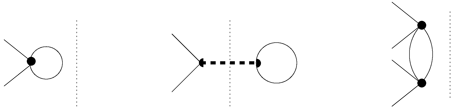
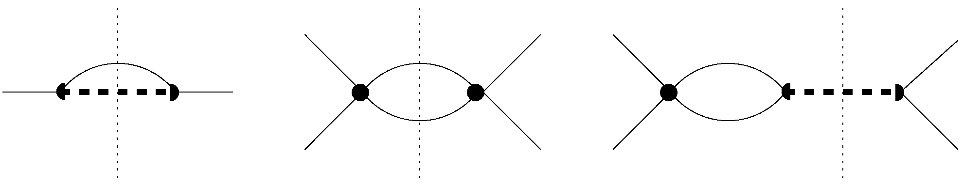
cf. Figure 3 and Figure 4 where the -dependent coefficients are
with and , . The higher than two-cluster contributions arising from the Neumann expansion have been ignored in deriving the beta functions. The integrations can been carried out analytically.
It is remarkable that the STP beta functions contain no open parameters; in other words, the STP parameters evolve as in the traditional STP formalism of Quantum Field Theory. This follows immediately from the equivalence of the inhomogeneous CTP and the STP graphs, mentioned in Section 2.4.
3.5. Separatrices and Phase Transition
A quantum phase transition corresponds to a separatrix of the renormalization group flow, indicating that small modifications of the theory in the UV lead to large changes in the IR. One cannot strictly establish a phase transition with the help of a truncated renormalization group flow but it is reasonable to assume that while stable flows of an appropriately truncated flow represent a good approximation of the exact case this does not hold for trajectories with IR singularity. In fact, the latter never occurs for the exact flow and suggests that important parameters are missed due to the limited ansatz space for the blocked action. Hence the trajectory on the border of the stable IR flow indicates a separatrix of the exact solution.
One can gain some qualitative insight into the scaling laws of the closed parameters by writing the first two equation of (39) as a single equation for ,
describing the complex trajectory of a one-dimensional damped motion with
in terms of the complex beta function parameters and . The quartic coupling is found by . It is instructive first to inspect this equation in simpler cases.
In an invariant Euclidean field theory the parameters are real and one finds at the subtraction point
and
The renormalized trajectory starting with the initial conditions , stretches toward negative . In the UV scaling regime, , , , and the evolution starting with positive velocity (towards decreasing t!) is slowed down by the friction. In the IR regime, , , , both the friction and the term continue to damp the evolution. However, for sufficiently negative the damped increase of may be slow enough to reach at . As this crossover is approached B diverges sending to zero and an IR singularity is generated.
In the real time theory with sharp momentum cutoff at the subtraction point one finds
and
The parameters remain real and the symmetry broken phase is recovered in a qualitatively similar manner as in the imaginary time case.
The evolution of the theory in Minkowski space-time defined by a plane wave subtraction point (28) with at the threshold, , is driven by
where
and the symmetry broken phase is recovered as well. The complex trajectory may avoid the singularity by having . A short enough finite life-time of the quasi particles may weaken the crossover singularity and render the simple ansatz for the action applicable in the IR region within the symmetry broken phase.
The evolution of the open parameters can be read off from the scale-dependence of satisfying the equation
corresponding to a one-dimensional particle of unit mass, moving under the influence of a friction force with Newton constant
and a potential
The real beta function parameters are -dependent, and . The other open parameter is given by . The trajectory starting in the vicinity of the Gaussian fixed point where with and . The dominant scale-dependence of C and D with finite is , which weakens the potential but keeps the friction stable and approximately scale invariant. The coordinate y rolls down on the potential in the positive direction reflecting the irreversible accumulation of the system-environment entanglement during the change of the cutoff. The entanglement is weak for short lived quasi particle excitations hence C and D decreases with increasing . Thus, the exponentially fast decreasing potential cannot destabilize the evolution for large enough . However, the lowering of strengthens the potential and the exponentially steep potential may make the trajectory divergent at finite scale, generating a separatrix for the flow of the open parameters. The evolution in the UV direction makes the instability stronger since .
4. Renormalization Group Flow
The issues we intend to comment on or clarify by the numerical integration of the evolution equations are (1) the phase structure of the theory, (2) the closed bare theory limit, (3) the relevance of the open parameters of the action and (4) the renormalizability. We do this by exploring the renormalization group flow restricted to initial conditions in the vicinity of the Gaussian fixed point.
4.1. Phase Structure
The closed parameters evolve independently from the open channels hence the usual phase transition between the symmetrical and the spontaneous broken phases takes place at the same place as in the closed theory. The singularity at is a spinodal instability indicating that the vacuum is in the symmetry broken phase [55,56,57,58,59]. The IR singularity of the open channels indicates that the theory may undergo a phase transition where the system-environment interactions increases abruptly for the IR modes.
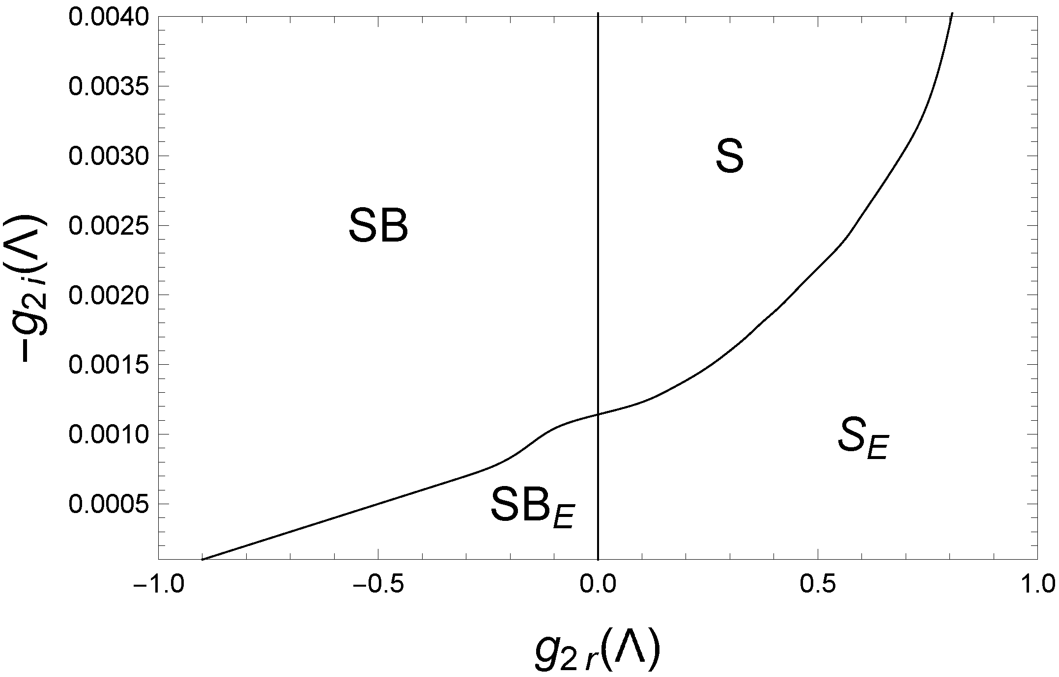
Such a phase structure is borne out by the integration of the evolution equations (39). The four phases are shown on the complex plane of Figure 5. The spontaneous breakdown of the symmetry is indicated within the framework of the local potential approximation by the divergence of the propagator, , followed by a spinodal instability as the cutoff is lowered. The transition between the symmetric and the symmetry broken phase is a slightly right bended vertical line. The phases with regular or divergent are separated by the curve which increases with .
When the quasi-particles are stable enough to interact with the environment, the theories below the curve, the evolution drives at finite cutoff. The large positive turns on the interactions with the environment indicating a large amount of system-environment entanglement generated by the lowering of the cutoff. Hence the phases under the curve are called symmetric or symmetry broken entangled phases. The exact renormalized trajectories are regular in the IR direction and the singularity in the entangled phase indicates the insufficiency of our ansatz to give account of the increased amount of entanglement. A safe conclusion, point (iii) of the introduction, is that the long range macroscopic dynamics turns suddenly non-perturbative in terms of the microscopical quasi-particles at the curve separating the upper and the lower phases. With an improved ansatz for the action which allows us to penetrate the entangled phase the lower end of the separation of the phases and should become visible since the STP parameters evolve independently from the open interactions.
The Lorentzian width of the subtraction point controls the energy interval around the where the contributions to the evolution of the running coupling constants are read off from the right hand side of Equation (27) and smaller width makes the propagating quasi-particles dominate. The general trend is that the entangled phase shrinks with the increase of , we need propagating quasi-particles to pick up the system-environment entanglement. The decrease of leads ultimately to numerical instabilities, c.f. Section 4.2. Among the initial conditions with reliable solution we found no example that the closed limit , cf. the inverse propagator (11), with would avoid the entangled phase.
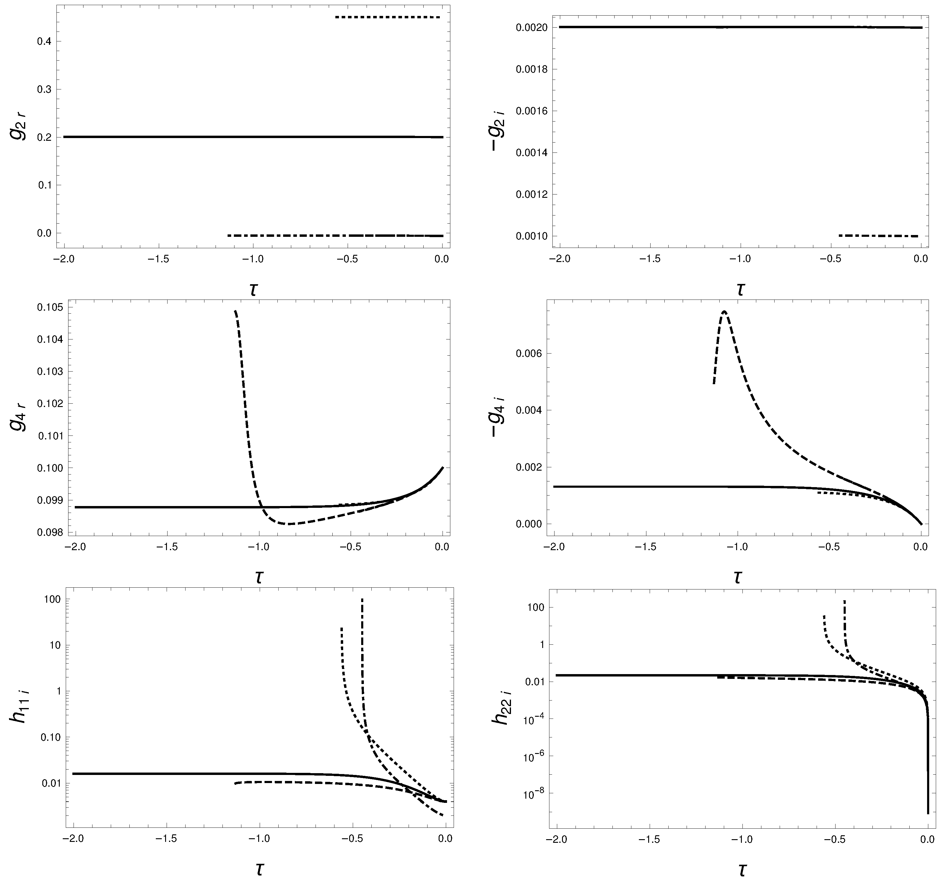
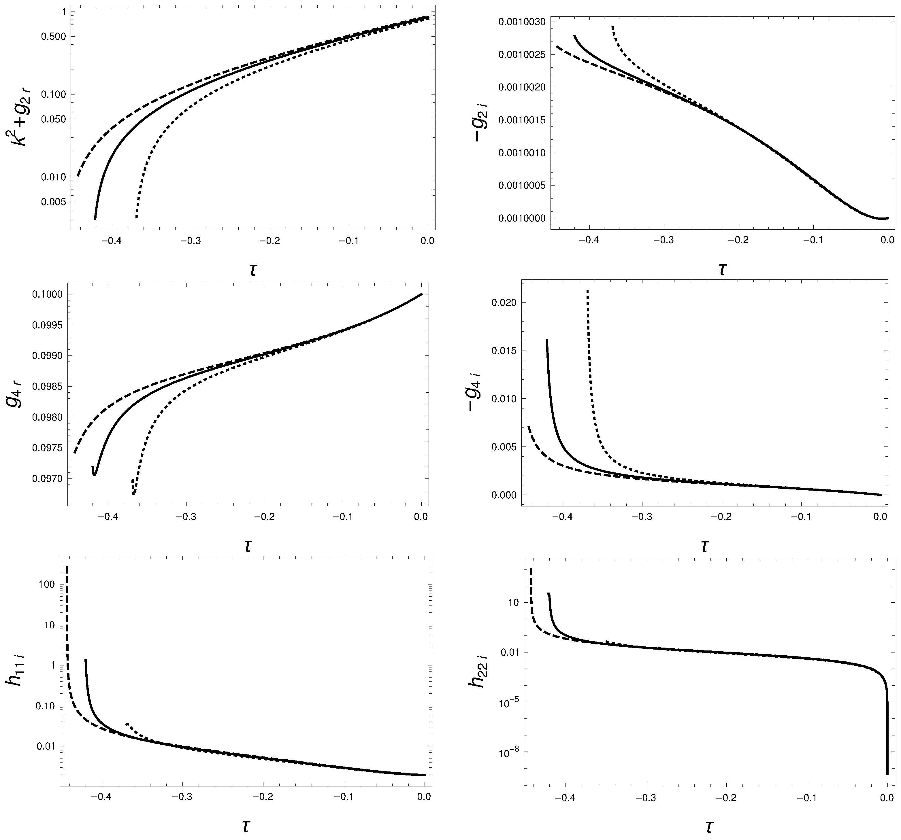
The typical trajectories, shown in Figure 6, indicate the presence of two independent phase transitions, one for the closed and the other for the open parameters. The left inequality of (19) is satisfied in the entangled phase indicating the presence of strong decoherence. A more detailed flow at the phase boundary is given in Figure 7. The strong increase of and in the phase before the evolution has to be halted indicates that the quasi particle become unstable at the onset of the spinodal instability. On the other side of the phase transition, in the phase, the singularity appears only in the open parameters.
4.2. Closed Initial Dynamics
The main message of this work is the necessity of using open quantum field theories and retaining the inevitable UV-IR entanglement during the renormalization; see point (i) in the Introduction. While it is well known that the system-environment entanglement plays a decisive role in open quantum dynamics this feature has not been followed in quantum field theory. One can already see from the qualitative picture of Section 3.5 that the movement with the cutoff either towards the IR or the UV direction leads to the accumulation of the entanglement contributions. A more detailed view of the generation of the mixed contributions to the blocked action can be found by inspecting the renormalization group flow in the limit of a closed initial theory, and .
Let us make a blocking step in a closed theory with infinitesimal when and consider the beta function of . The energy flowing through the third Feynman graph of Figure 3 is or . The integrand of the loop integral with integral variable contains two propagators with energies and in the second line of Equation (40). The imaginary Dirac-delta peaks of the propagators, written by the help of the identity , coincide for , at and generate an imaginary contribution to the beta function. The same holds for however the imaginary part drops to when . Such a threshold singularity renders the subtraction point dominated by the propagating particles, , difficult to use numerically.
One can avoid the threshold singularity by the use of a subtraction point with finite which is a wave packet rather that a monochromatic wave. The coinciding poles of the closed theory still generate imaginary contribution to the beta functions of and but the dependence on the subtraction point, on the parameter, is now regular. We could follow the trajectories down to with and being at least around 10 however the roundoff errors in the initial phase of the evolution arising from the incomplete cancellation between the partial fractions of the loop integral make the trajectory unreliable beyond this limit.
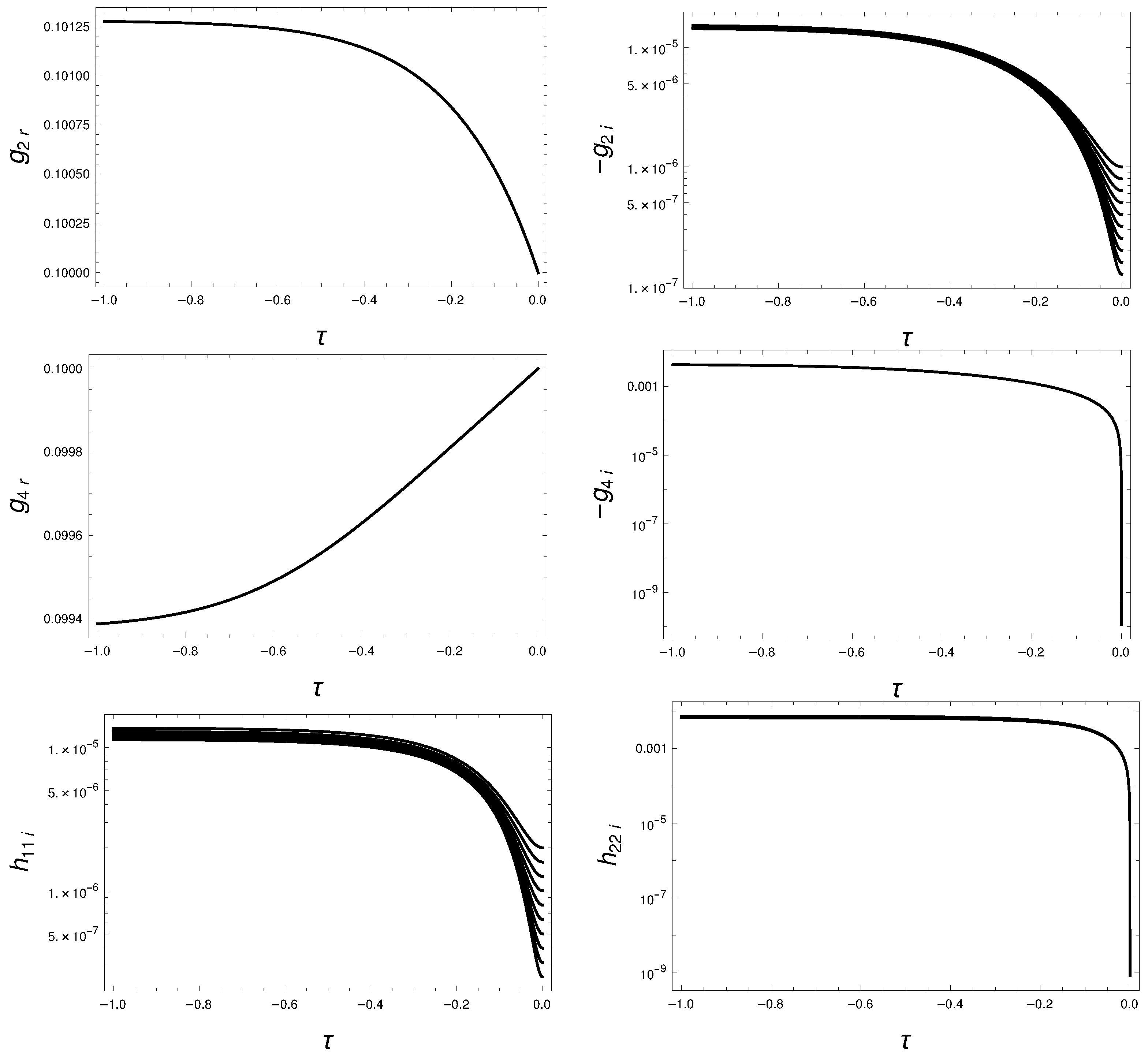
The renormalized trajectory of the symmetric non-entengled phase is shown as and is decreased in Figure 8. The limit is best tested by the convergence of or . The almost vertical evolution of and , the parameters with vanishing initial condition, is an artifact of the logarithmic plot. In terms of elementary processes, the second graph of Figure 4 drives a rapid increase of by starting in a closed theory which feeds back to accelerate the increase of the originally infinitesimal . These two processes are represented by the coefficient of the exponential function in the potential (51).
4.3. Relevance of Open Channels
The second quantitative point showing the importance of the open interaction channels consists of an estimate of their impact on the expectation values of physical quantities. Here we face the issue of the relevance of the IR-UV entanglement for observables defined at a scale far below the cutoff scale where the observed system and its environment are separated. A simple power counting argument indicates that the parameters and are renormalizable and therefore should be kept in the action.
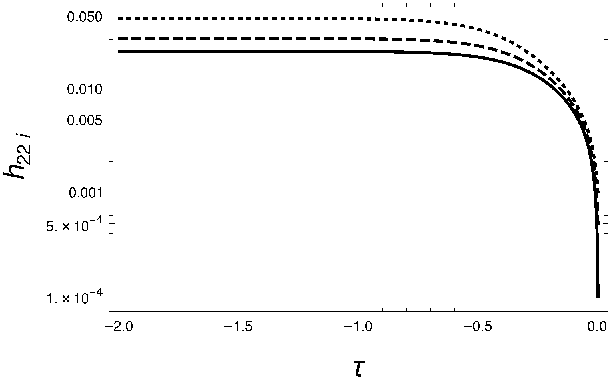
A more detailed view of the mixed contributions to the blocked action can be found by inspecting the renormalized trajectory. The open channels bring in new two parameters into the action, and . The former is relevant (super renormalizable) according to power counting. The latter is marginal and higher order contributions make it relevant or irrelevant (non-renormalizable). To see what happens, we followed the evolution of corresponding to initial conditions where only its initial condition was slightly changed around zero. The trajectories plotted on Figure 9 correspond to the initial conditions and their increasing separation in the UV scaling regime indicates the relevance of this coupling constant, as in point (ii) of the Introduction.
4.4. Towards the UV
Finally, a few words about the UV direction and the issue of renormalizability. The conditions of renormalizability can be imposed on four, increasingly restrictive, levels. (i) The cutoff can be sent to infinity without encountering divergences. The perturbative condition is given by power counting and the model of our ansatz belongs to this class. (ii) The renormalization conditions, a set of non-linear equations, are soluble for the bare parameters. These conditions are violated in non-asymptotically free theories which are restricted to free theories as the cutoff is removed. The simple qualitative view of the renormalization group flow of the open parameters, mentioned in Section 3.5, suggests an UV Landau pole for since the friction term with its “wrong”, unstable sign sends to infinity at finite scale. (iii) The last condition can be strengthened by requiring the stability of the dynamics. The stability is expressed in terms of inequalities for the imaginary parts of some running parameters, which are specially difficult to maintain. All the trajectories encountered in our numerical efforts to follow the theory in the UV direction led to a condensate, , or to the violation of the stability conditions. (iv) The cutoff is assumed to be very large in the multiplicative renormalization group scheme where the contributions, proportional to a negative powers of the cutoff, are neglected. This approximation is untenable in effective theories where the possibility of placing freely the cutoff to higher energy is assured by requiring the absence of the UV Landau pole. Since the functional renormalization group method handles all contribution within the restricted functional space it is better suited to test the renormalizability.
One can see without going into the details that the renormalization procedure and the interpretation of possible UV fixed points of open theories remains a challenging open question at the present time.
5. Summary
The functional renormalization group equation of the four-dimensional model is discussed here to clarify the importance of the open channels of a quantum field theory. The solution of the evolution equation is sought within a rather simple functional space for the action where the local vertices in space are kept up to fourth order in the field with the minimal necessary time dependence for the open channels. Furthermore, the absence of condensate is assumed in deriving the evolution equation.
It is argued that open interactions arise when the cutoff is moved either in the UV or the IR direction. Furthermore, it is found that the open parameters of the action are relevant around the Gaussian fixed point. Thus, closed theories are simply excluded from considerations by requiring an adjustable separation between the observed IR and the unresolved UV degrees of freedom.
Another result which is important in establishing a relation between the macroscpic and the microscopic physics is that our simple model exhibits a non-perturbative relation between the microscopic (UV) and the strongly decohered macroscopic (IR) degrees of freedom within a closed or almost closed system. Thus, one cannot take the correspondence principle between the classical and the quantum degrees of freedom for granted.
These results obviously raise further questions. An obvious issue is the systematic extension of the anstaz space for the action and the check of the stability of these results. This direction requires the use of multi-local actions [60] and the increase of the order of the truncation in the field amplitude. Another question is the boost invariance. The separation of the degrees of freedom into IR and UV classes is based on the de Broglie wavelength and is not boost invariant. Furthermore, there is a conflict between regulators and boost symmetry since the latter has infinite volume [61]. Hence the question arises whether Lorentz symmetry can be maintained in a quantum field theory at any scale. Furthermore, the obvious importance of the system-environment entanglement in open dynamics results in the spectacular success of quantum field theory, by ignoring the open interaction channels rather surprising. A revisiting of the renormalization program of realistic models is needed to locate the mechanism which operates in certain observations and suppresses the UV-IR entanglement.
Author Contributions
Conceptualization, S.N. and J.P.; writing—review and editing, S.N. and J.P. All authors have read and agreed to the published version of the manuscript.
Funding
This research received no external funding.
Institutional Review Board Statement
Not applicable.
Informed Consent Statement
Not applicable.
Conflicts of Interest
The authors declare no conflict of interest.
References
- Schwinger, J. Brownian motion of a quantum oscillator. J. Math. Phys. 1961, 2, 407–432. [Google Scholar] [CrossRef]
- Schwinger, J. Particles and Sources; Addison-Wesley: Cambridge, MA, USA, 1970; Volume 1–3. [Google Scholar]
- Keldysh, L.V. Diagram technique for nonequilibrium processes. Sov. Phys. JETP 1965, 20, 1018. [Google Scholar]
- Zeh, H.D. On the interpretation of measurement in quantum theory. Found. Phys. 1970, 1, 69–76. [Google Scholar] [CrossRef]
- Zurek, W.H. Pointer basis of quantum apparatus: Into what mixture does the wave packet collapse? Phys. Rev. D 1981, 24, 1516–1525. [Google Scholar] [CrossRef]
- Joos, E.; Zeh, H.D. The emergence of Classical Properties through Interaction with the Environment. Z. Phys. B 1985, 59, 223–243. [Google Scholar] [CrossRef]
- Zurek, W.H. Reduction of the Wavepacket: How Long Does it Take? In Frontiers of Nonequilibrium Statistical Physics; Moore, G.T., Scully, M.O., Eds.; Plenum Press: New York, NY, USA, 1986; pp. 145–150. [Google Scholar]
- Gell-Mann, M.; Hartle, J.B. Classical equations for quantum systems. Phys. Rev. D 1993, 47, 3345–3382. [Google Scholar] [CrossRef] [Green Version]
- Griffiths, R.B. Consistent Historoes and the Interpretation of Quantum Mechanics. J. Stat. Phys. 1984, 36, 219–272. [Google Scholar] [CrossRef]
- Omnès, R. Logical reformulation of quantum mechanics. I. Foundations. J. Stat. Phys. 1988, 53, 893–932. [Google Scholar] [CrossRef]
- Halliwell, J.J. A review of the decoherent histories approach to quantum mechanics. arXiv 1994, arXiv:gr-qc/9407040. [Google Scholar]
- Kamenev, A. Field Theory of Non-Equilibrium Systems; Cambridge University Press: Cambridge, UK, 2011. [Google Scholar]
- Rammer, J. Quantum Field Theory of Non-Equilibrium States; Cambridge University Press: Cambridge, UK, 2007. [Google Scholar]
- Weiss, U. Quantum Dissipative Systems; World Scientific: Singapore, 1993. [Google Scholar]
- Zaikin, A.D.; Golubev, D.S. Dissiative Quantum Mechanics of Nanostructures; Jenny Stanford: Singapore, 2019. [Google Scholar]
- Sieberer, L.M.; Buchhold, M.; Diehl, S. Keldysh field theory for open driven quantum systems. Rep. Prog. Phys. 2016, 79, 096001. [Google Scholar] [CrossRef]
- Bertini, B.; Heidrich-Meisner, F.; Karrasch, C.; Prosen, T.; Steinigeweg, R.; Žnidarič, M. Finite-temperature transprot in one-dimensional quantum lattice models. Rev. Mod. Phys. 2021, 93, 025003. [Google Scholar] [CrossRef]
- Umezawa, H.; Matsumoto, H.; Tachiki, M. Thermo Field Dynamics and Condensed States; North Holland: Amsterdam, The Netherlands, 1982. [Google Scholar]
- Calzetta, E.A.; Hu, B.L.A. Nonequilibrium Quantum Field Theory; Cambridge University Press: Cambridge, UK, 2008. [Google Scholar]
- Feynman, R.P.; Vernon, F.L. The Theory of a General Quantum System Interacting with a Linear Dissipative System. Ann. Phys. 1963, 24, 118–173. [Google Scholar] [CrossRef] [Green Version]
- Lombardo, F.; Mazzitelli, F.D. Coarse graining and decoherence in quantum field theory. Phys. Rev. D 1996, 53, 2001–2011. [Google Scholar] [CrossRef] [PubMed] [Green Version]
- Dalvit, D.A.R.; Mazzitelli, F.D. Exact CTP renormalization group equation for the coarse grained effective action. Phys. Rev. D 1996, 54, 6338–6346. [Google Scholar] [CrossRef] [Green Version]
- Anastopoulos, C. Coarse grainings and irreversibility in quantum field theory. Phys. Rev. D 1997, 56, 1009–1020. [Google Scholar] [CrossRef] [Green Version]
- Gezzi, R.; Pruschke, T.; Meden, V. Functional renormalization group for nonequilibrium quantum many-body problems. Phys. Rev. B 2007, 75, 045324. [Google Scholar] [CrossRef] [Green Version]
- Mitra, A.; Takei, S.; Kim, Y.B.; Millis, A.J. Nonequilibrium Quantum Criticality in Open Electronic Systems. Phys. Rev. Lett. 2006, 97, 236808. [Google Scholar] [CrossRef] [Green Version]
- Jakobs, S.G.; Meden, V.; Schoeller, H. Nonequilibrium Functional Renormalization Group for Interacting Quantum Systems. Phys. Rev. Lett. 2007, 99, 150603. [Google Scholar] [CrossRef] [Green Version]
- Zanella, J.; Calzetta, E. Renormalization group study of damping in nonequilibrium field theory. arXiv 2006, arXiv:hep-th/0611222. [Google Scholar]
- Zanella, J.; Calzetta, E. Inflation and nonequilibrium renormalization group. J. Phys. A 2007, 40, 7037–7041. [Google Scholar] [CrossRef] [Green Version]
- Calzetta, E.A.; Hu, B.L.; Mazzitelli, F.D. Coarse grained effective action and renormalization group theory in semiclassical gravity and cosmology. Phys. Rep. 2001, 352, 459–520. [Google Scholar] [CrossRef] [Green Version]
- Bergerhoff, B.; Reingruber, J. Thermal renormalization group equations and the phase transition of scalar O(N) theories. Phys. Rev. D 1999, 60, 105036. [Google Scholar]
- Canet, L.; Chaté, H. Non-perturbative Approach to Critical Dynamics. J. Phys. A 2007, 40, 1937–1950. [Google Scholar] [CrossRef] [Green Version]
- Mesterházy, D.; Stockemer, J.H.; Palhares, L.F.; Berges, J. Dynamic universality class of Model C from the functional renormalization group. Phys. Rev. B 2013, 88, 174301. [Google Scholar] [CrossRef] [Green Version]
- Sieberer, L.M.; Huber, S.D.; Altman, E.; Diehl, S. Dynamical Critical Phenomena in Driven-Dissipative Systems. Phys. Rev. Lett. 2013, 110, 195301. [Google Scholar] [CrossRef] [PubMed] [Green Version]
- Gasenzer, T.; Berges, J.; Schmidt, M.G.; Seco, M. Nonperturbative dynamical many-body theory of a Bose–Einstein condensate. Phys. Rev. A 2005, 72, 063604. [Google Scholar] [CrossRef] [Green Version]
- Berges, J.; Gasenzer, T. Quantum versus classical statistical dynamics of an ultracold Bose gas. Phys. Rev. A 2007, 76, 033604. [Google Scholar] [CrossRef] [Green Version]
- Sieberer, L.M.; Huber, S.D.; Altman, E.; Diehl, S. Nonequilibrium functional renormalization for driven-dissipative Bose–Einstein condensation. Phys. Rev. B 2014, 89, 134310. [Google Scholar] [CrossRef] [Green Version]
- Pawlowski, J.M.; Strodthoff, N. Real time correlation functions and the functional renormalization group. Phys. Rev. D 2015, 92, 094009. [Google Scholar] [CrossRef] [Green Version]
- Huelsmann, S.; Schlichting, S.; Scior, P. Spectral functions from the real-time functional renormalization group. Phys. Rev. D 2020, 102, 096004. [Google Scholar] [CrossRef]
- Kasper, V.; Hebenstreit, F.; Berges, J. Fermion production from real-time lattice gauge theory in the classical-statistical regime. Phys. Rev. D 2014, 90, 025016. [Google Scholar] [CrossRef] [Green Version]
- Zanella, J.; Calzetta, E. Renormalization group and nonequilibrium action in stochastic field theory. Phys. Rev. E 2002, 66, 036134. [Google Scholar] [CrossRef] [Green Version]
- Nagy, S.; Polonyi, J.; Steib, I. Quantum renormalization group. Phys. Rev. D 2016, 93, 025008. [Google Scholar] [CrossRef] [Green Version]
- Berges, J.; Hoffmeister, G. Nonthermal fixed points and the functional renormalization group. Nucl. Phys. B 2009, 813, 383–407. [Google Scholar] [CrossRef] [Green Version]
- Gasenzer, T.; Pawlowski, J. Towards far-from-equilibrium quantum field dynamics: A functional renormalisation-group approach. Phys. Lett. B 2008, 670, 135–140. [Google Scholar] [CrossRef] [Green Version]
- Gasenzer, T.; Kessler, S.; Pawlowski, J. Far-from-equilibrium quantum many-body dynamics. Eur. Phys. J. C 2010, 70, 423–443. [Google Scholar] [CrossRef] [Green Version]
- Corell, L.; Cyrol, A.K.; Heller, M.; Pawlowski, J.M. Flowing with the temporal renormalization group. Phys. Rev. D 2021, 104, 025005. [Google Scholar] [CrossRef]
- Baidya, A.; Jana, C.; Loganayagam, R.; Rudra, A. Renormalization in Open Quantum Field Theory I: Scalar field theory. JHEP 2017, 11, 204. [Google Scholar] [CrossRef] [Green Version]
- Baidya, A.; Jana, C.; Loganayagam, R.; Rudra, A. Renormalisation in Open Quantum Field theory II: Yukawa theory and PV reduction. arXiv 2019, arXiv:1906.10180. [Google Scholar]
- Ostrogradsky, M. Mémoires sur les équations différentielles, relatives au problème des isopérimètres. Mem. Acad. St. Petersbourg 1850, 6, 385–517. [Google Scholar]
- Woodard, R.P. Ostrogradsky’s theorem on Hamiltonian instability. Scholarpedia 2015, 10, 32243. [Google Scholar] [CrossRef]
- Wegner, F.J.; Houghton, A. Renormalization group equation for critical phenomena. Phys. Rev. A 1973, 8, 401–412. [Google Scholar] [CrossRef]
- Polonyi, J. Classical and quantum effective theories. Phys. Rev. D 2014, 90, 065010. [Google Scholar] [CrossRef] [Green Version]
- Polonyi, J. Spontaneous Breakdown of the Time Reversal Symmetry. Symmetry 2016, 8, 25. [Google Scholar] [CrossRef] [Green Version]
- Polonyi, J.; Rachid, I. Equilibrium particle states in weakly open dynamics. arXiv 2019, arXiv:1904.06338. [Google Scholar]
- Steib, I.; Nagy, S.; Polonyi, J. Renormalization in Minkowski space-time. Int. J. Mod. Phys. A 2021, 36, 2150031. [Google Scholar] [CrossRef]
- Tetradis, N.; Wetterich, C. The high temperature phase transition for ϕ4 theories. Nucl. Phys. B 1993, 398, 659–696. [Google Scholar] [CrossRef]
- Caillol, J.M. The non-perturbative renormalization group in the ordered phase. Nucl. Phys. B 2012, 855, 854–884. [Google Scholar] [CrossRef] [Green Version]
- Paláez, M.; Wschebor, N. Ordered phase of the O(N) model within the nonperturbative renormalization group. Phys. Rev. E 2016, 94, 042136. [Google Scholar] [CrossRef] [Green Version]
- Alexandre, J.; Branchina, V.; Polonyi, J. Instability Induced Renormalization. Phys. Lett. B 1999, 445, 351–356. [Google Scholar] [CrossRef] [Green Version]
- Pangon, V.; Nagy, S.; Polonyi, J.; Sailer, K. Symmetry breaking and the functional RG scheme. Int. J. Mod. Phys. A 2011, 26, 1327–1345. [Google Scholar] [CrossRef] [Green Version]
- Nagy, S.; Polonyi, J.; Steib, I. Euclidean scalar field theory in the bi-local approximation. Phys. Rev. D 2018, 97, 085002. [Google Scholar]
- Polonyi, J. Boost invariant regulator for field theories. Int. J. Mod. Phys. A 2019, 34, 1950017. [Google Scholar] [CrossRef]
Figure 1.
A solid line stands for the propagator in a CTP Feynman graph. The vertical dotted line separates the ket and the bra sectors where the field variable and are used, respectively. The time runs upward. (a) The Wightman function connects the bra and the ket components. (b) An alternative representation of the Wightman function where the lines follow the world lines of the excitations until the final time when the trace operation carried out in (6) connect them. These excited states are on-shell.

Figure 2.
An inhomogeneous Feynman graph contributing to a sixth order Green function of the field . The subgraphs and belong to ket and bra excitations, respectively. (a) The sum of the energies flowing into is vanishing hence at least on of the line carries negative energy and the graph is vanishing. (b) The alternative representation with the lines indicating the excitations contributing to the trace. This process is suppressed if the energy is vanishing at the initial time.

Figure 3.
The Feynman graphs contributing to the STP parameters. The horizontal dashed line connects the two clusters of the bi-local vertices which couple the bra and the ket.
Figure 3.
The Feynman graphs contributing to the STP parameters. The horizontal dashed line connects the two clusters of the bi-local vertices which couple the bra and the ket.

Figure 4.
The Feynman graphs contributing to the CTP parameters. The time inverted version of the last graph enters, as well.
Figure 4.
The Feynman graphs contributing to the CTP parameters. The time inverted version of the last graph enters, as well.

Figure 5.
The phase structrure on the complex plane at , , and , S: symmetrical phase, SB: symmetry broken phase and the entengled phases with the subscript E.
Figure 5.
The phase structrure on the complex plane at , , and , S: symmetrical phase, SB: symmetry broken phase and the entengled phases with the subscript E.

Figure 6.
Typical trajectories at , , in the phases S (, continuous line), (, dashed line), (, dotted line) and (, dashed-dotted line), .
Figure 6.
Typical trajectories at , , in the phases S (, continuous line), (, dashed line), (, dotted line) and (, dashed-dotted line), .

Figure 7.
Zooming into the phase boundary. The trajectories in the (dotted line) and (dashed line) phases together with the separatrix (continuous line) belong to the initial conditions (dashed line), (solid line), (dotted line), , , , and .
Figure 7.
Zooming into the phase boundary. The trajectories in the (dotted line) and (dashed line) phases together with the separatrix (continuous line) belong to the initial conditions (dashed line), (solid line), (dotted line), , , , and .

Figure 8.
The closed limit, , followed in the interval in the symmetric phase at , , , , .

Figure 9.
Scaling of the open parameters at , , , (solid line), (dashed line), (dotted line), .

Publisher’s Note: MDPI stays neutral with regard to jurisdictional claims in published maps and institutional affiliations. |
© 2022 by the authors. Licensee MDPI, Basel, Switzerland. This article is an open access article distributed under the terms and conditions of the Creative Commons Attribution (CC BY) license (https://creativecommons.org/licenses/by/4.0/).
Share and Cite
MDPI and ACS Style
Nagy, S.; Polonyi, J. Renormalizing Open Quantum Field Theories. Universe 2022, 8, 127. https://doi.org/10.3390/universe8020127
AMA Style
Nagy S, Polonyi J. Renormalizing Open Quantum Field Theories. Universe. 2022; 8(2):127. https://doi.org/10.3390/universe8020127
Chicago/Turabian StyleNagy, Sandor, and Janos Polonyi. 2022. "Renormalizing Open Quantum Field Theories" Universe 8, no. 2: 127. https://doi.org/10.3390/universe8020127
Note that from the first issue of 2016, this journal uses article numbers instead of page numbers. See further details here.