
A 2D Lithospheric Magnetic Anomaly Field over Egypt Using Gradient Data of Swarm Mission

1
Physics Department, Faculty of Science, Fayoum University, Fayoum 63514, Egypt
2
National Research Institute of Astronomy and Geophysics (NRIAG), Helwan 11421, Egypt
3
Institute of Geophysics and Geoinformatics, TU Bergakademie Freiberg, 09599 Freiberg, Germany
*
Author to whom correspondence should be addressed.
Universe 2022, 8(10), 530; https://doi.org/10.3390/universe8100530
Submission received: 23 August 2022
/
Revised: 8 October 2022
/
Accepted: 9 October 2022
/
Published: 12 October 2022
(This article belongs to the Section Space Science)
Abstract
:The current work makes use of the geometrical configuration of the two lower-altitude Swarm satellites (Swarm A and C), moving side by side with a longitudinal distance of 1.4°, to estimate a two-dimensional (2D) model of the lithospheric magnetic anomaly field over Egypt using gradient data. The gradient in both the north–south and the east–west directions have been inverted using the weighted damping least-squares fit technique to estimate the best model coefficients of the 2D model. The best model coefficients have been obtained under the expansion of the Legendre polynomial from degree n = 7 to n = 56. Results showed that the gradient of the field in the north–south direction is always much smoother than that in the east–west direction. The noise in the east–west direction is attributed to the different environmental conditions surrounding both satellites. The modeled field always showed smoother variations than the observed data, even for the horizontal components (Bx and By).
1. Introduction
The lithosphere is the crust and the upper layer of the mantle. It consists of rocks that can be broken into plates and causes plate tectonics [1]. These rocks are characterized by different magnetic susceptibilities [2]. Their magnetism depends on their mineral compositions. The magnetic field from these rocks is denoted as the lithospheric magnetic anomaly field [3,4,5]. The separation of the lithospheric magnetic anomaly field requires good-quality magnetic data because the magnetic field observed on the Earth’s surface is an ensemble made up of different sources (the Earth’s core, lithosphere, and external fields due to the currents of the ionosphere and the magnetosphere) [6]. The main goal of modelling the lithospheric magnetic field is achieving a high-resolution model free of (external) noise to map the subsurface geological structure [7,8]. To obtain a high-resolution model, there are different approaches for separating the lithospheric magnetic field using ground-based and space-based magnetic data [9]. These approaches are divided into local/regional and global modelling techniques. The most common global models that separate the lithospheric magnetic field are CHAOS [10], MF [11], and the comprehensive model (CM) [9,12,13]. The CHAOS series is one of the most updated models. It collects data from ground-based observatories, Ørsted, CHAMP [14], SAC-C, CryoSat-2, and Swarm satellites [15]. CHAOS calculates the main, lithosphere, and external fields during quiet periods. It uses a sophisticated selection criterion to reduce external noise [16]. This model has been derived using the quietest data when the Sun is at least 10° below the horizon. The spherical harmonic degrees of the CHAOS model reach 130 and 133 at the altitudes of 400 km and 300 km, respectively [11,17]. The coefficients of the CHAOS model are regularly updated every 4 to 6 months, according to the observed data of Swarm satellite [10]. The spherical harmonic expansion of the CHAOS model, up to degree 133, corresponds to a spatial resolution of 300 km [18]. The CM model is derived from data collected from ground-based observatories and the Ørsted, SAC-C, CHAMP, and Swarm satellites. The CM model calculates oceanic tidal magnetic sources, ionospheric quiet-time fields, and the induction fields of both the ionosphere and the magnetosphere, in addition to internal and external fields [9,12,13]. The lithospheric field is expanded up to spherical harmonic degree 120, corresponding to the resolution of 333 km [13]. The magnetic anomaly field with short-scale wavelength is not applicable to the global models because it requires a high degree of expansion that makes the computation intensive. Therefore, regional approaches have been used for modelling the lithospheric field, such as spherical cap harmonic analysis (SCHA) [19], 2D models, and rectangular harmonic analysis (RHA) [20,21]. However, these models give accurate anomaly field data in a short-scale wavelength with a lower order than global models. There are shortcomings regarding the use of these local field models. The first problem with the SCHA model is the difficulty in separating the internal and external fields from each other [22] because both are expanded in terms of the potential function at the surface of the cap. Second, in order to reach a high spatial resolution, we must use a small cap (dense grid); subsequently, a large expansion must be implemented. Therefore the computation is very intense and requires a long time to reach convergence [23]. Third, the edge effect problem is considered a common issue in all local models that could be overcome by enlarging the area under study [24]. Additionally, RHAs produce unrealistic values when expanding non-cyclic data [25,26]. This problem could be overcome through expanding the lithospheric field data to a polynomial [26].
The current work makes use of 8 years of magnetic data recorded by Swarm A and C to model the lithospheric magnetic anomaly field over Egypt and its surroundings, using a 2D model built on Legendre polynomials. Unlike [27], we use gradient magnetic data to obtain an accurate model because gradient data is less affected by external noise [17]. The results presented by [28] neglect the analysis of the lithospheric anomaly of the component because this component was very noisy, more than the Bx component. Therefore, in the current work, we have tried to model the whole components using the gradient data from the lower-altitude Swarm satellites. The structure of the current work is as follows: Section 2 presents the data set and the selection criteria in addition to a theoretical discussion of the modelling techniques. Section 3 presents the results of our method in weighted and non-weighted inverted means. Finally, Section 4 presents our conclusions.
2. Data Set and Methodology
2.1. Data Set and Selection Criterion
The Swarm mission consists of three satellites (Alpha, Bravo, and Charlie) used to study the Earth’s geomagnetic field [28,29]. The mission was launched on 25 November 2013 to study the ionospheric current systems and model the Earth’s magnetic field [30]. Swarm A and C are flying side-by-side, separated by 1.4° (~150 km) at an altitude of 400 km, while Swarm B is flying at an altitude of 520 km with a higher inclination angle than Swarm A and C [6]. Our study depends on the Swarm A and C satellites. We have used MAGx_LR Level 1b Swarm data, which is available on the European Space Agency (ESA) website (https://swarm-diss.eo.esa.int/ (accessed on 31 December 2021)). We have used the quiet-time magnetic data recorded by the two lower-altitude Swarm satellites, A and C, from January 2014 until August 2021. These data have been used to model the lithospheric magnetic anomaly field over Egypt and its surroundings. The quiet-time Swarm magnetic data has been selected according to the following criteria:
- 1)
- Local nighttime data ().
- 2)
- Kp 1.
- 3)
- The interplanetary magnetic field (IMF) within .
- 4)
- The disturbance storm time index within −20 < Dst < 20 daily values.
- 5)
- The regional data observed within [] latitude and [] longitudes with observational error < 0.3 nT.
The geomagnetic indices and solar wind parameters were obtained from the Omni website (https://omniweb.gsfc.nasa.gov/form/dx4.html (accessed on 31 December 2021)). Figure 1 illustrates the relationship between the altitude and the number of data points within each 2 km. It shows that the maximum number of data points are collected at an altitude of about 440 km. Therefore, we have selected observations where the satellite is located within km. These altitudinal limits have also been chosen to overcome the altitudinal variation of the lithospheric magnetic anomaly field.
The gradient data from these satellites (Swarm A and C) have been calculated in the north–south (N–S) and the east–west (E–W) directions. It is worth noting that, we have first subsampled the 1 s into a 10 s time resolution. We have avoided subsampling it to 30 s in order to overcome gaps because the resolution of our plotted maps is 1° × 1° (latxlon). Subsequently, we have followed the same criteria set as [17] in calculating the gradient data by confirming that the time lag between the two satellites (Swarm A and C) does not exceed the 50 s. Therefore, any path where Swarm A and Swarm C lagged by more than 50 s was excluded from the analysis. The N–S gradient data were calculated by subtracting two points separated by 15 s as observed by the same satellite [17]. Therefore, the amount of N–S gradient data is twice as large as the amount of E–W gradient data.
2.2. Modeling Techniques
The lithospheric magnetic anomaly field () was calculated after the subtraction of the core () and the external ( CHAOS fields from the observed data (), which is represented mathematically according to Equation (1):
where is a vector of the lithospheric magnetic anomaly field in the three (x, y, z) geographic coordinates according to the coordinates of the observed data. Subsequently, we subtracted the lithospheric magnetic anomaly field between Swarm A and Swarm C, which represents the E–W gradient data. In addition, we subtracted the lithospheric magnetic anomaly field between two points separated by 15 s along the path of the same satellite, which represents the N–S gradient data. The three vector components of the gradient data through this work will be mathematically represented in the forms , , and . To model the gradient magnetic field data in two dimensions, we expanded it in terms of the Legendre polynomial function (). According to [27,31], the 2D model can be represented mathematically according to Equation (2):
where is the index of the data points, and is any vector of gradient magnetic anomaly field data. Each observed point (i) has and , denoting the latitude and longitude, respectively, where and are the intermediate coordinates between any two points used for calculating the gradient data. The mathematical representation of both and is defined by Equations 3.1 and 3.2 of [31]. It is worth noting that the selection of an intermediate location between any two points used for deriving gradient data, or even the location of either of these points, does not change the final results. Parameter is defined as the coefficients of the 2D model. These model coefficients could be represented mathematically as vector and are defined as . In this work, we have used the orders of expansion of the Legendre polynomials n = 7–56. More details regarding the determination of the limits of expansion of the Legendre polynomial are explained within the context of the current work. Equation (2) can be written in a mathematical, compact form using the matrix , as shown in Equation (3):
where is the operator matrix of the Legendre polynomial as defined in [27].
The weighted damped least-squares fit method used to estimate the model coefficients can be represented mathematically according to Equation (4):
where is the weight matrix that has diagonal elements equal to , and is the standard deviation of the gradient data [17]. More details regarding the calculation of the standard deviation of the analyzed data are given in the context of the current work. Parameter is the damping parameter, and is a unitary diagonal matrix.
The resolution matrix (R) of the weighted damped least-squares fit method is given by Equation (5):
Figure 2 illustrates the relationship between the norm of the model coefficients (m) and the standard deviation of the misfit of the N–S gradient [32,33]. The misfit has been calculated according to [17]. The black, red, blue, and green lines correspond to the trade-off curves of , , and , respectively, where is the gradient of the total lithospheric magnetic field. The values of the damping parameters for each trade-off curve are in the order We have chosen the damping parameter , which locates at the knee of the trade-off curves [32,33].
Figure 3 shows the diagonal elements of the resolution matrix R with respect to the parameter numbers of of the N–S gradient data at the best damping parameter (). It shows that the diagonal element of the resolution matrix approaches unity, which demonstrates the great description of the model for the data. The increase of R at higher orders could be interpreted in terms of the dominance of the noise at higher orders of expansion [27,33].
In order to truncate the model to a certain degree, we have studied the spectrum of the model [] as shown in Figure 4a. It shows that the spectrum increases from degree 0 to degree 7 and then decreases again from 7 to 60. Figure 4b is similar to Figure 4a but on a logarithmic scale. The horizontal dashed line in Figure 4b corresponds to the spectrum of value equal to zero at degree 56. According to [15], the initial degrees from 0 to 7 correspond to fields from a source region other than the lithospheric magnetic field, while the degrees from 7 to 56 correspond to the lithospheric magnetic field. Therefore, we have expanded our data from degree 7 up to 56, and subsequently, the vector model coefficients become of length 1625.
3. Results and Discussions
Figure 5 shows the standard deviation of the N–S gradient field components. The standard deviation data binned to regions of the surface area of 2.5 degrees. For each binned area, the standard deviation has been calculated as shown in Figure 5 for the component. It shows regions of higher standard deviation corresponding to large errors in the data. The same calculations have been performed for the other vector field components, , , and , respectively. According to Equation (4), each data point located within a specific binned region has been divided by its corresponding standard deviation. This process has been implemented by several users to reduce the effect of outlier points [34,35].
The non-gradient lithospheric magnetic field data presented by [27] is more affected by external sources/noise. It exhibited N–S stripes in the X-component, especially at higher altitudes. To reduce this noise, we used gradient data from a Swarm satellite [36].
Figure 6 shows the E–W gradient data calculated from Swarm A and C. Rows from top to bottom correspond to the , , , and components, respectively. Columns from left to right correspond to observed, modeled, and weighted modeled gradient data, respectively. The observed and are noisier than and . The noise in the horizontal components ( and ) could be attributed to external sources. In addition, we can interpret it in terms of the sensitivity of the data sets onboard the Swarm A and Swarm C satellites. In order to reduce this noise, we have implemented the weighted damped least-squares technique as shown in the most right column of Figure 6. It is worth noting that the magnetic anomaly in the component was excluded from [27] because the non-gradient data are strongly affected by external and lithospheric activities (e.g., Earthquakes, ionospheric dynamos, etc.). However, using the gradient data is a powerful technique in removing external noise in comparison with [27], which is strongly affected by external ionospheric and magnetospheric noise. The weighted damping least-squares fit technique of the gradient data has the capability to emphasize a lithospheric magnetic anomaly in a much smoother form, especially in the and components. The weighted damped modeled data in the and components illustrated magnetic anomalies that could not clearly be seen in the observed gradient data in most left panels. The most clearly enhanced anomalies under the weighted damping technique are shown in the northwest and in the middle of the map of the component. The field strength of these regions is enhanced under the action of the damping technique in comparison with the observed lithospheric gradient data.
Figure 7 is similar to Figure 6, but for the N–S gradient; data was observed from both Swarm A and Swarm C. The upper, middle, and lower rows correspond to the N–S , , and components, respectively. Columns from left to right correspond to the observed, modeled, and weighted modeled data, respectively. It is clearly shown that both the and components show no significant differences between the observed gradient data and our weighted modeled data, while both the and modelled (weighted and non-weighted) components have a smoother variation than the observed data. Additionally, Figure 7 shows that the observed N–S gradient data does not contain N–S strips, as appeared in the E–W data, which means the N–S gradient is generally less affected by external fields in comparison with the E–W gradient data.
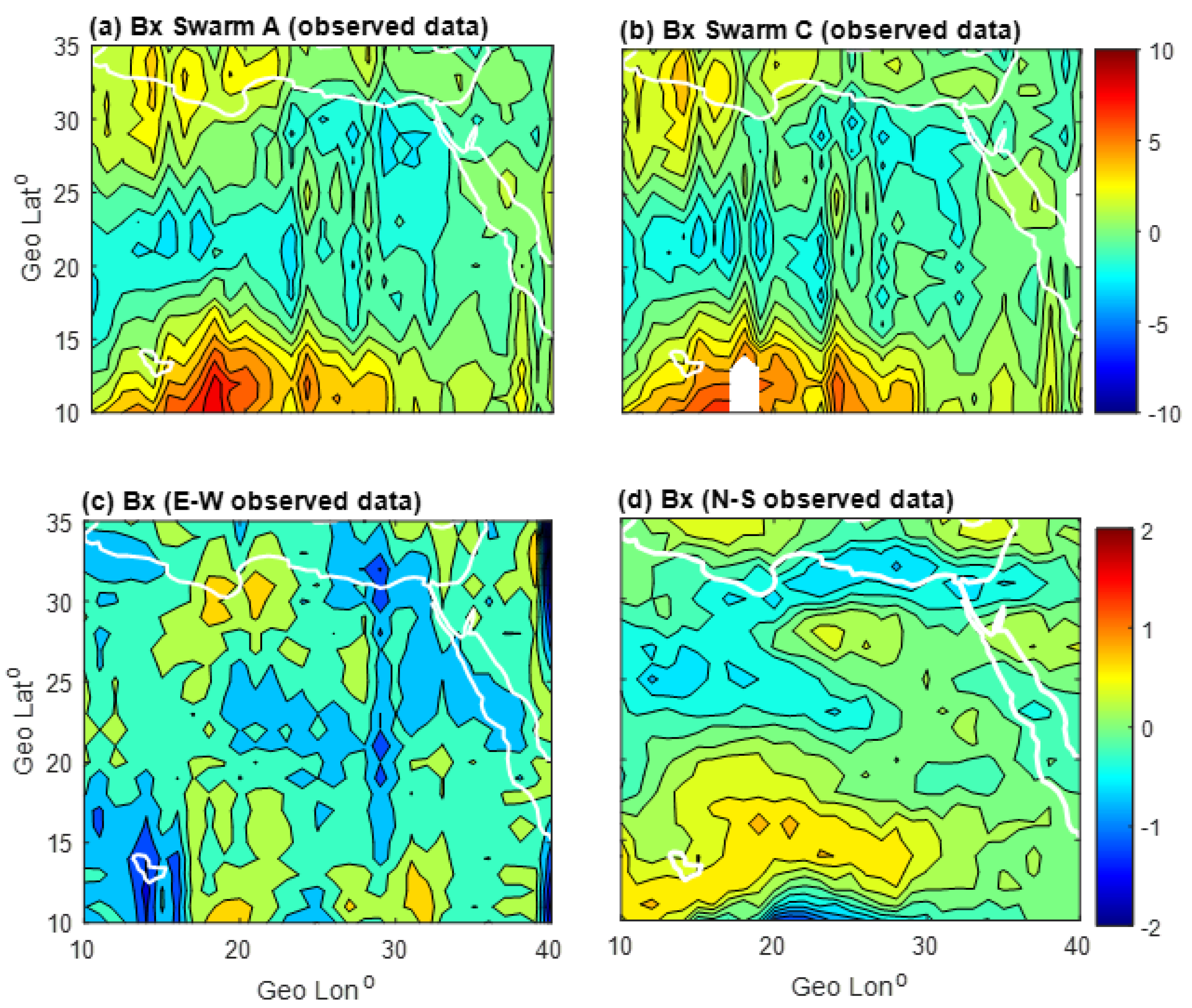
In order to emphasize the capability of the gradient technique in overcoming external noise, especially that which exists in the horizontal components (), we have conducted a comparison between the gradient data in the N–S and E–W directions, as shown in Figure 8c,d, respectively. Figure 8a,b clearly shows that the non-gradient data observed by Swarm A shows differences in comparison with the non-gradient data observed by Swarm C; in addition, both satellites have N–S strips. However, the satellites contain the same exact data sets; these differences could be interpreted in terms of the difference in environmental conditions surrounding the satellites because Swarm A and Swarm C are separated horizontally by 150 km distance in longitude. The N–S gradient data is less affected by this problem (different environmental conditions) because we have subtracted two points observed by the same satellite, so the mechanical and electronical noise, in addition to the environmental conditions, is canceled through the subtraction process. So, subtracting Swarm A and Swarm C magnetic data to obtain the E–W gradient resulted in noisy maps, in comparison with the N–S gradient data, as is clearly shown by comparing the images in Figure 8c,d.
4. Conclusions
The current work makes use of 8 years (from January 2014 to August 2021) of magnetic field data observed by two lower-altitude satellites (Swarm A and C) of the Swarm constellation to model the lithospheric magnetic anomaly field over Egypt and the surrounding area. The data selected according to our criteria of quiet-time conditions and within km of the altitude of 440 km have been chosen to overcome the altitudinal variation of the field. To make use of the geometrical configuration of the two lower-altitude satellites, the gradients of the field in the N–S and the E–W directions have been calculated. The observed E–W gradient data, derived from the differences between Swarm A and C, exhibited a noisier map than did the N–S gradient data. This could be attributed to the different environmental conditions surrounding the two satellites (Swarm A and C), as the satellites are separated by ~150 km distance in longitude.
In order to reduce the noise of the observed data, a weighted damped least-squares fit technique of a 2D model has been adopted. In this model, we have implemented the Legendre polynomial to model the gradient of the lithospheric magnetic anomaly data. To solve this model, we have expanded the field in terms of the Legendre polynomial from degree 7 to degree 56. These limits of expansion degrees have been chosen according to the spectrum of the model at the best damping parameter. The best damping parameter at the knee of the trade-off curve for our solved model equals . The weighted damped least-squares fit method of the 2D model has greatly reduced the effects of ionospheric and magnetospheric noise sources in both the N–S gradient and E–W gradient directions. The anomaly model derived starting from gradient data is of higher quality than the one reported by [27], which is based on non-gradient data.
Author Contributions
Conceptualization, E.G. and A.F.; methodology, A.A. and A.F.; software, A.A. and A.F.; validation, A.A., E.G., M.S. and A.F.; formal analysis, A.A. and A.F.; investigation, E.G. and A.F.; resources, A.A.; data curation, A.A. and A.F.; writing—original draft preparation, A.A. and A.F.; writing—review and editing, A.A., E.G., M.S. and A.F. All authors have read and agreed to the published version of the manuscript.
Funding
This research received no external funding.
Data Availability Statement
Swarm magnetic data has been downloaded from the following website: (https://swarm-diss.eo.esa.int/) accessed date is 31 December 2021, and the magnetic activity data has been downloaded from the following website: (https://omniweb.gsfc.nasa.gov/form/dx4.html) accessed date is 31 December 2021.
Acknowledgments
We would like to thank the European Space Agency (ESA) for providing us with the low-resolution magnetic data observed by the Swarm satellite (https://swarm-diss.eo.esa.int/ (accessed on 31 December 2021)) and the Omni website (https://omniweb.gsfc.nasa.gov/form/dx4.html (accessed on 31 December 2021)) for providing us with the geomagnetic indices and solar wind parameters.
Conflicts of Interest
The authors declare no conflict of interest.
References
- Cawood, P.A.; Kroner, A.; Pisarevsky, S. Precambrian plate tectonics: Criteria and evidence. GSA Today 2006, 16, 4. [Google Scholar] [CrossRef] [Green Version]
- Mandea, M.; Korte, M. Geomagnetic Observations and Models; Springer: Berlin/Heidelberg, Germany, 2010; Volume 5. [Google Scholar]
- Milligan, P.; Petkovic, P.; Drummond, B. Potential-field datasets for the Australian region: Their significance in mapping basement architecture. Spec. Pap. Geol. Soc. Am. 2003, 372, 129–140. [Google Scholar]
- Hemant, K.; Maus, S. Geological modeling of the new CHAMP magnetic anomaly maps using a geographical information system technique. J. Geophys. Res. Solid Earth 2005, 110, 1–23. [Google Scholar] [CrossRef]
- Maus, S. An ellipsoidal harmonic representation of Earth’s lithospheric magnetic field to degree and order 720. Geochem. Geophys. Geosystems 2010, 11. [Google Scholar] [CrossRef] [Green Version]
- Olsen, N.; Friis-Christensen, E.; Floberghagen, R.; Alken, P.; Beggan, C.D.; Chulliat, A.; Doornbos, E.; Da Encarnação, J.T.; Hamilton, B.; Hulot, G. The Swarm satellite constellation application and research facility (SCARF) and Swarm data products. Earth Planets Space 2013, 65, 1189–1200. [Google Scholar] [CrossRef]
- Bloxham, J.; Jackson, A. Time-dependent mapping of the magnetic field at the core-mantle boundary. J. Geophys. Res. Solid Earth 1992, 97, 19537–19563. [Google Scholar] [CrossRef]
- Jackson, A.; Jonkers, A.R.; Walker, M.R. Four centuries of geomagnetic secular variation from historical records. Philos. Trans. R. Soc. London. Ser. A Math. Phys. Eng. Sci. 2000, 358, 957–990. [Google Scholar] [CrossRef]
- Sabaka, T.J.; Olsen, N.; Purucker, M.E. Extending comprehensive models of the Earth’s magnetic field with Ørsted and CHAMP data. Geophys. J. Int. 2004, 159, 521–547. [Google Scholar] [CrossRef]
- Finlay, C.C.; Kloss, C.; Olsen, N.; Hammer, M.D.; Tøffner-Clausen, L.; Grayver, A.; Kuvshinov, A. The CHAOS-7 geomagnetic field model and observed changes in the South Atlantic Anomaly. Earth Planets Space 2020, 72, 1–31. [Google Scholar] [CrossRef]
- Thébault, E.; Lesur, V.; Kauristie, K.; Shore, R. Magnetic Field Data Correction in Space for Modelling the Lithospheric Magnetic Field. Space Sci. Rev. 2017, 206, 191–223. [Google Scholar] [CrossRef]
- Sabaka, T.J.; Olsen, N.; Langel, R.A. A comprehensive model of the quiet-time, near-Earth magnetic field: Phase 3. Geophys. J. Int. 2002, 151, 32–68. [Google Scholar] [CrossRef]
- Sabaka, T.J.; Tøffner-Clausen, L.; Olsen, N.; Finlay, C.C. CM6: A comprehensive geomagnetic field model derived from both CHAMP and Swarm satellite observations. Earth Planets Space 2020, 72, 1–24. [Google Scholar] [CrossRef]
- Reigber, C.; Lühr, H.; Schwintzer, P. CHAMP mission status. Adv. Space Res. 2002, 30, 129–134. [Google Scholar] [CrossRef]
- Olsen, N.; Lühr, H.; Finlay, C.C.; Sabaka, T.J.; Michaelis, I.; Rauberg, J.; Tøffner-Clausen, L. The CHAOS-4 geomagnetic field model. Geophys. J. Int. 2014, 197, 815–827. [Google Scholar] [CrossRef]
- Russell, J.; Shiells, G.; Kerridge, D. Reduction of Well-Bore Positional Uncertainty Through Application of a New Geomagnetic In-Field Referencing Technique. In Proceedings of the SPE Annual Technical Conference and Exhibition, Dallas, TX, USA, October 1995. [Google Scholar]
- Olsen, N.; Ravat, D.; Finlay, C.C.; Kother, L.K. LCS-1: A high-resolution global model of the lithospheric magnetic field derived from CHAMP and Swarm satellite observations. Geophys. J. Int. 2017, 211, 1461–1477. [Google Scholar] [CrossRef] [Green Version]
- Alken, P.; Maus, S.; Chulliat, A.; Manoj, C. NOAA/NGDC candidate models for the 12th generation International Geomagnetic Reference Field. Earth Planets Space 2015, 67, 1–9. [Google Scholar] [CrossRef] [Green Version]
- De Santis, A.; Battelli, O.; Kerridge, D. Spherical cap harmonic analysis applied to regional field modelling for Italy. J. Geomagn. Geoelectr. 1990, 42, 1019–1036. [Google Scholar] [CrossRef]
- Alldredge, L. Rectangular harmonic analysis applied to the geomagnetic field. J. Geophys. Res. Solid Earth 1981, 86, 3021–3026. [Google Scholar] [CrossRef]
- Nakagawa, I.; Yukutake, T. Rectangular harmonic analyses of geomagnetic anomalies derived from MAGSAT data over the area of the Japanese Islands. J. Geomagn. Geoelectr. 1985, 37, 957–977. [Google Scholar] [CrossRef] [Green Version]
- Haines, G. Computer programs for spherical cap harmonic analysis of potential and general fields. Comput. Geosci. 1988, 14, 413–447. [Google Scholar] [CrossRef]
- Thébault, E.; Schott, J.; Mandea, M.; Hoffbeck, J. A new proposal for spherical cap harmonic modelling. Geophys. J. Int. 2004, 159, 83–103. [Google Scholar] [CrossRef]
- Jiang, T.; Li, J.; Dang, Y.; Zhang, C.; Wang, Z.; Ke, B. Regional gravity field modeling based on rectangular harmonic analysis. Sci. China Earth Sci. 2014, 57, 1637–1644. [Google Scholar] [CrossRef]
- Malin, S.; Düzgit, Z.; Baydemir, N. Rectangular harmonic analysis revisited. J. Geophys. Res. Solid Earth 1996, 101, 28205–28209. [Google Scholar] [CrossRef]
- Düzgit, Z.; Baydemir, N.; Malin, S. Rectangular polynomial analysis of the regional geomagnetic field. Geophys. J. Int. 1997, 128, 737–743. [Google Scholar] [CrossRef] [Green Version]
- Fathy, A.; Ghamry, E. A two-dimensional lithospheric magnetic anomaly field model of Egypt using the measurements from swarm satellites. Geod. Geodyn. 2021, 12, 229–238. [Google Scholar] [CrossRef]
- Olsen, N.; Haagmans, R.; Sabaka, T.J.; Kuvshinov, A.; Maus, S.; Purucker, M.E.; Rother, M.; Lesur, V.; Mandea, M. The Swarm End-to-End mission simulator study: A demonstration of separating the various contributions to Earth’s magnetic field using synthetic data. Earth Planets Space 2006, 58, 359–370. [Google Scholar] [CrossRef] [Green Version]
- Friis-Christensen, E.; Lühr, H.; Hulot, G. Swarm: A constellation to study the Earth’s magnetic field. Earth Planets Space 2006, 58, 351–358. [Google Scholar] [CrossRef] [Green Version]
- Alken, P. Observations and modeling of the ionospheric gravity and diamagnetic current systems from CHAMP and Swarm measurements. J. Geophys. Res. Space Phys. 2016, 121, 589–601. [Google Scholar] [CrossRef] [Green Version]
- Zhang, J.; Yang, X.; Yan, J.; Wu, X. An analysis of the characteristics of crustal magnetic anomaly in China based on CHAMP satellite data. Geod. Geodyn. 2018, 9, 328–333. [Google Scholar] [CrossRef]
- Holme, R.; Bloxham, J. The magnetic fields of Uranus and Neptune: Methods and models. J. Geophys. Res. Planets 1996, 101, 2177–2200. [Google Scholar] [CrossRef] [Green Version]
- Gubbins, D.; Bloxham, J. Geomagnetic field analysis—III. Magnetic fields on the core—mantle boundary. Geophys. J. Int. 1985, 80, 695–713. [Google Scholar] [CrossRef]
- Kotsiaros, S.; Finlay, C.; Olsen, N. Use of along-track magnetic field differences in lithospheric field modelling. Geophys. J. Int. 2015, 200, 880–889. [Google Scholar] [CrossRef]
- Morschhauser, A.; Lesur, V.; Grott, M. A spherical harmonic model of the lithospheric magnetic field of Mars. J. Geophys. Res. Planets 2014, 119, 1162–1188. [Google Scholar] [CrossRef] [Green Version]
- Kotsiaros, S.; Olsen, N. The geomagnetic field gradient tensor. GEM-Int. J. Geomath. 2012, 3, 297–314. [Google Scholar] [CrossRef]
Figure 1.
The number of data points with altitude, with the maximum data point concentrated at an altitude of 440 km.
Figure 1.
The number of data points with altitude, with the maximum data point concentrated at an altitude of 440 km.
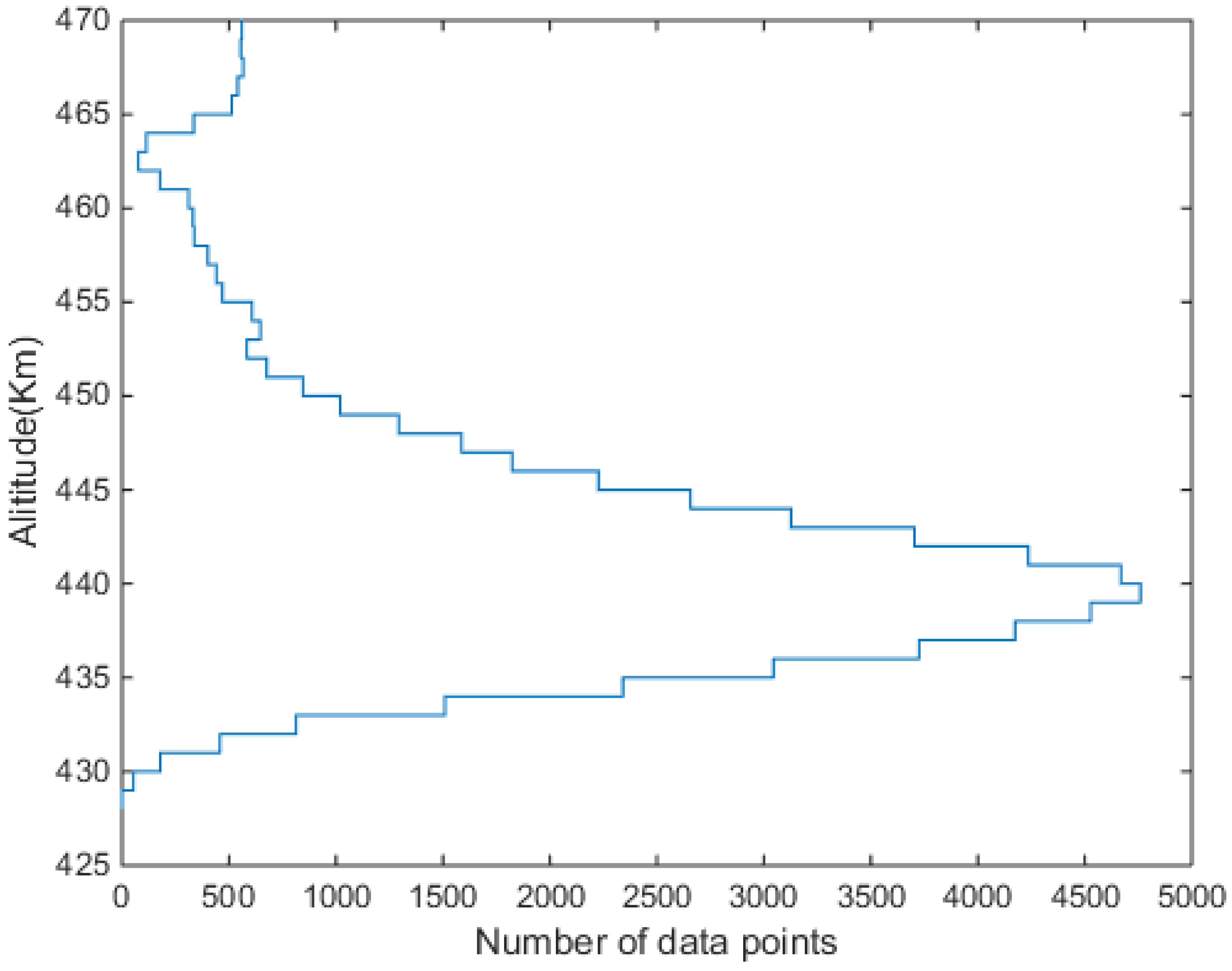
Figure 2.
The trade-off curve of the north–south , , , and . The variation of the norm (m) with respect to the standard deviation () of the misfit shows that the knee of the curve is located at the damping parameter, equaling .
Figure 2.
The trade-off curve of the north–south , , , and . The variation of the norm (m) with respect to the standard deviation () of the misfit shows that the knee of the curve is located at the damping parameter, equaling .
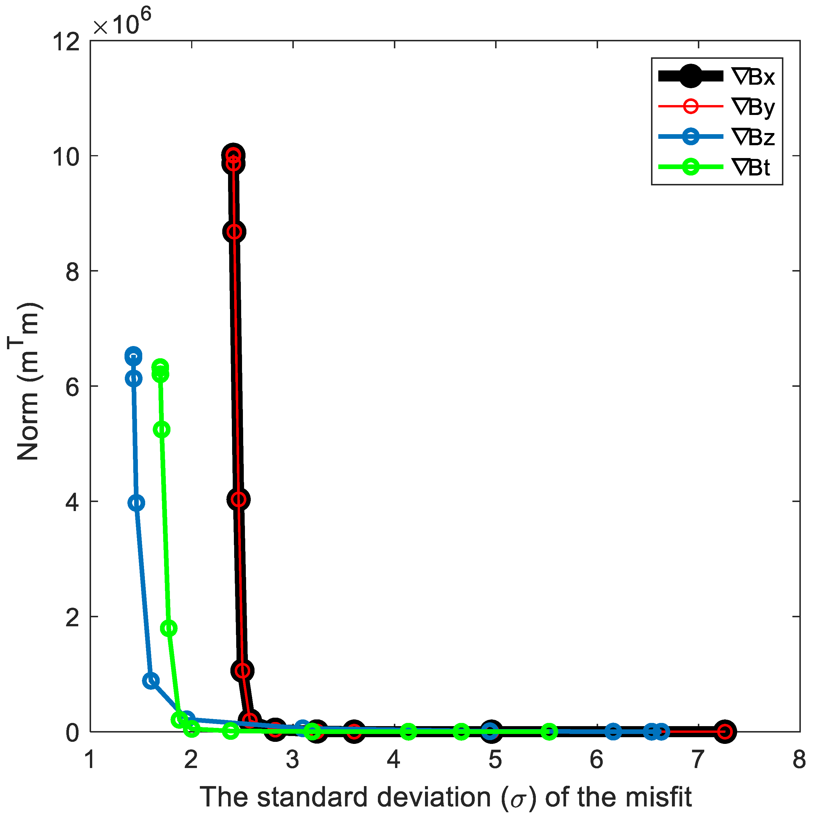
Figure 3.
The diagonal elements of the resolution matrix at damping parameter with respect to the parameter numbers.
Figure 3.
The diagonal elements of the resolution matrix at damping parameter with respect to the parameter numbers.
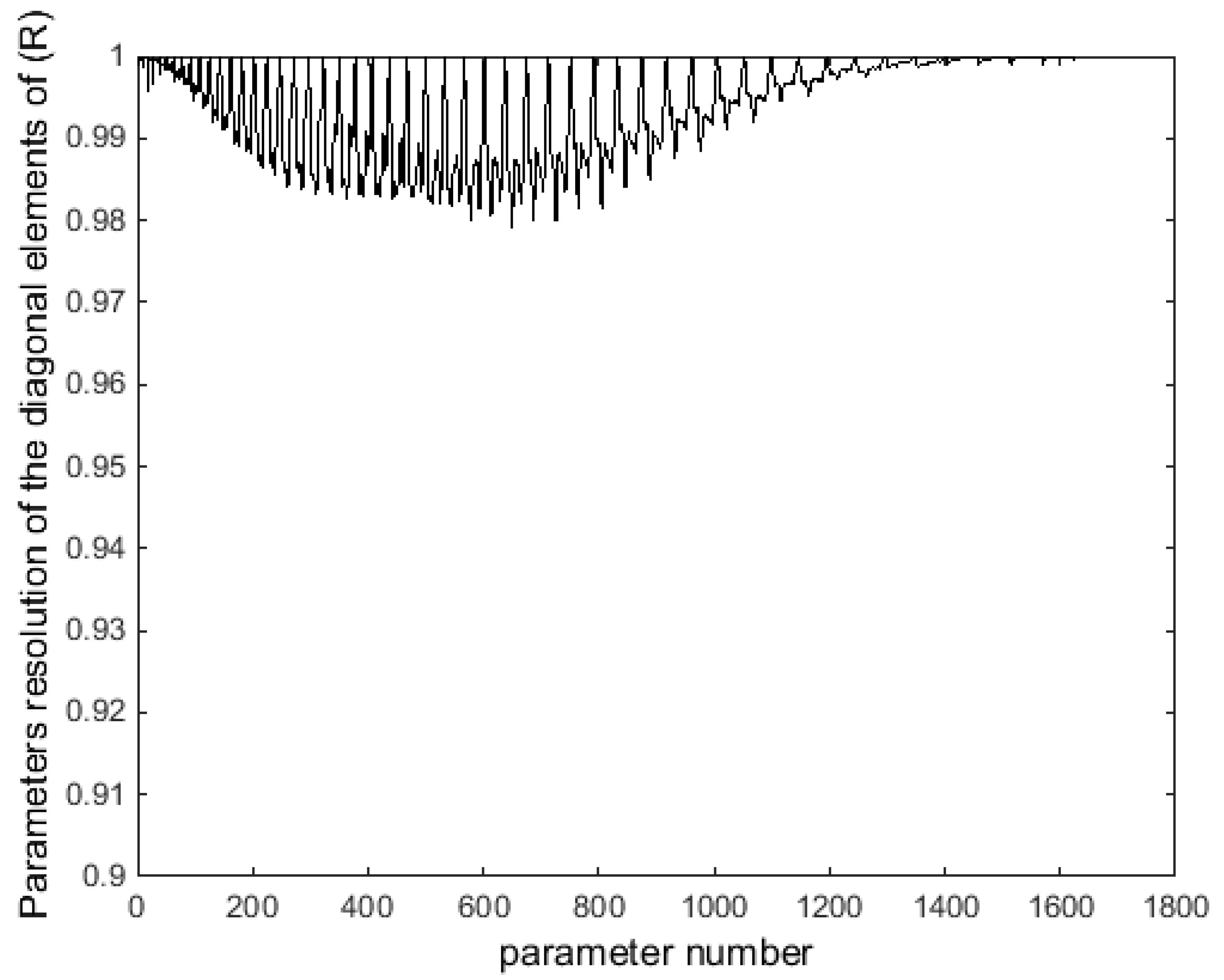
Figure 4.
The power spectrum of the model with respect to the degree (n), (a) in a linear scale and (b) in a logarithmic scale.
Figure 4.
The power spectrum of the model with respect to the degree (n), (a) in a linear scale and (b) in a logarithmic scale.
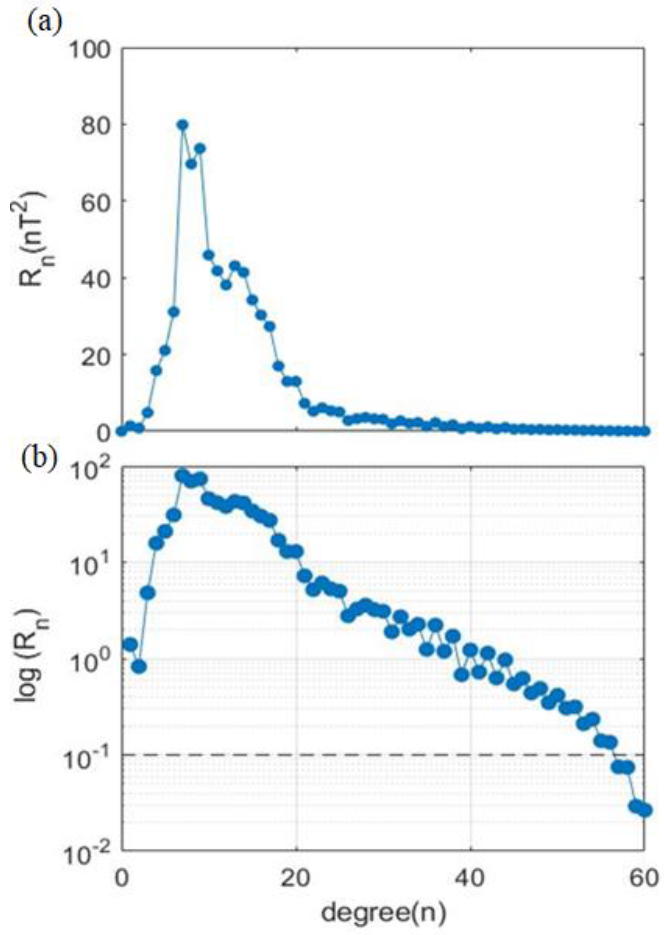
Figure 5.
The standard deviation of the N–S gradient field component binned to regions of the surface area of 2.5 degrees.
Figure 5.
The standard deviation of the N–S gradient field component binned to regions of the surface area of 2.5 degrees.
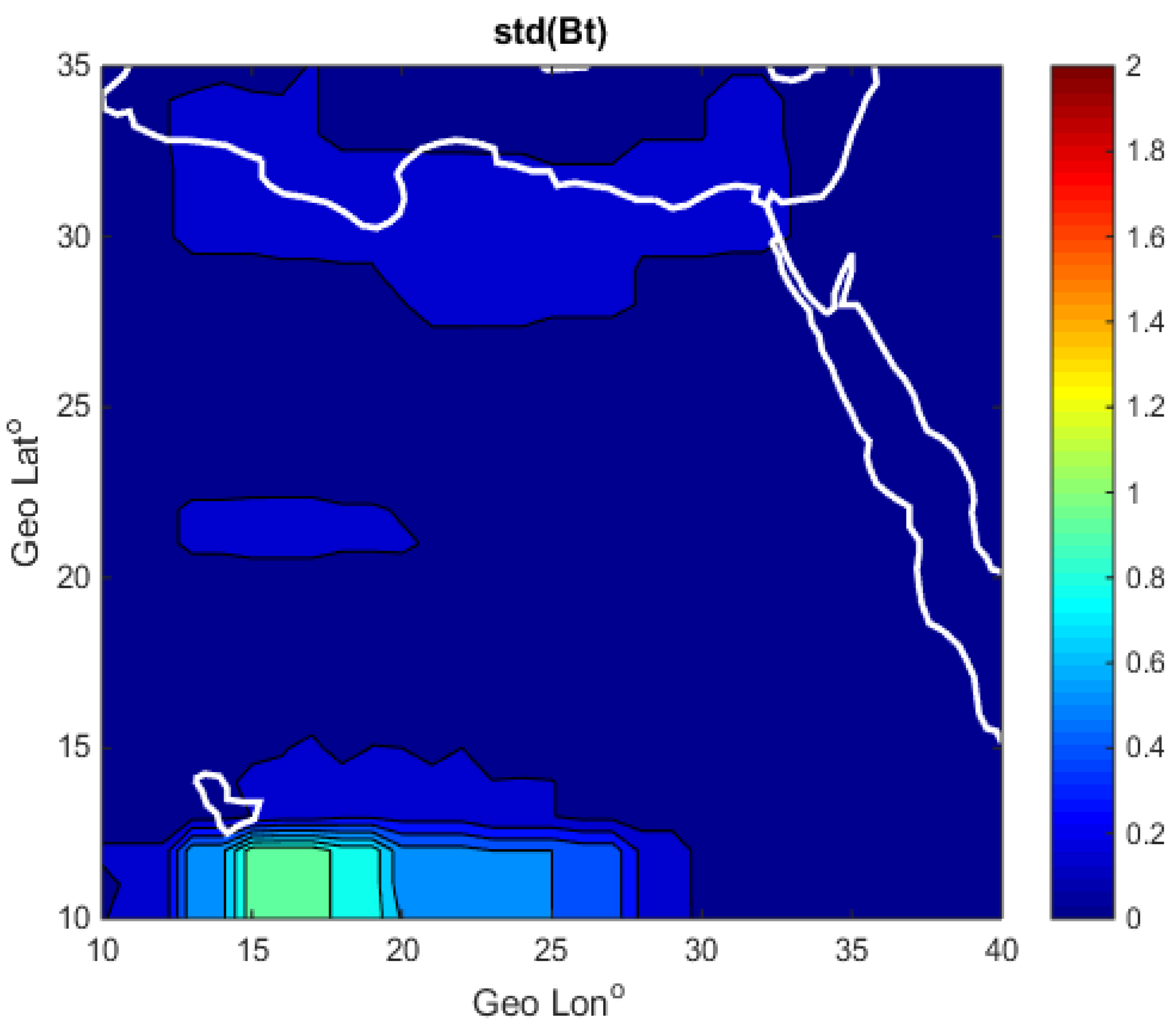
Figure 6.
The , , and components of E–W direction for the observed, modeled, and weighted modeled.

Figure 7.
Same like Figure 6 but for N-S direction.
Figure 7.
Same like Figure 6 but for N-S direction.
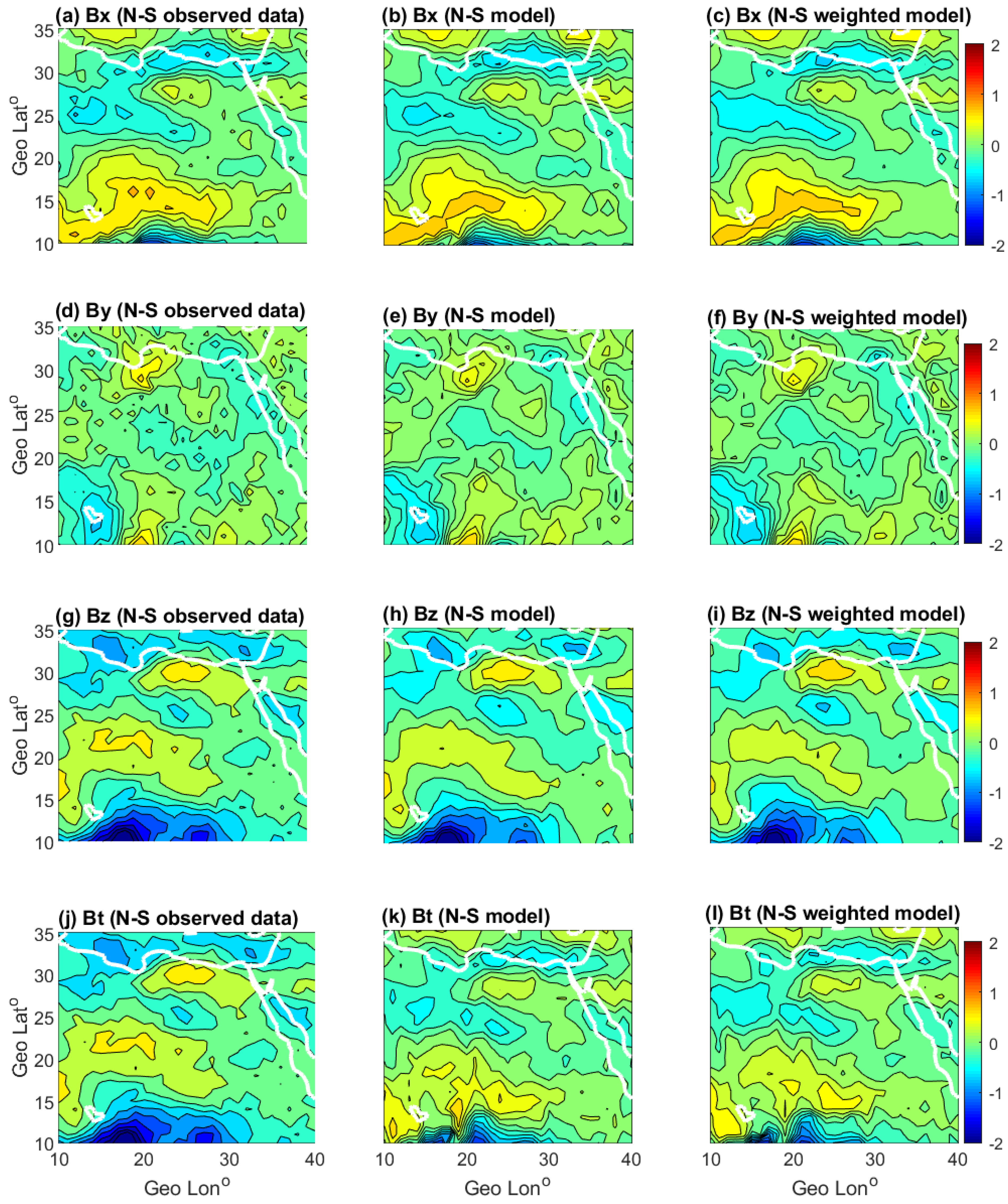
Figure 8.
The lithospheric magnetic anomaly field of the Bx component (a) observed by Swarm A, (b) observed by Swarm C, (c) gradient in the E–W direction, and d) gradient in the N–S direction.
Figure 8.
The lithospheric magnetic anomaly field of the Bx component (a) observed by Swarm A, (b) observed by Swarm C, (c) gradient in the E–W direction, and d) gradient in the N–S direction.
Publisher’s Note: MDPI stays neutral with regard to jurisdictional claims in published maps and institutional affiliations. |
© 2022 by the authors. Licensee MDPI, Basel, Switzerland. This article is an open access article distributed under the terms and conditions of the Creative Commons Attribution (CC BY) license (https://creativecommons.org/licenses/by/4.0/).
Share and Cite
MDPI and ACS Style
Abdellatif, A.; Ghamry, E.; Sobh, M.; Fathy, A. A 2D Lithospheric Magnetic Anomaly Field over Egypt Using Gradient Data of Swarm Mission. Universe 2022, 8, 530. https://doi.org/10.3390/universe8100530
AMA Style
Abdellatif A, Ghamry E, Sobh M, Fathy A. A 2D Lithospheric Magnetic Anomaly Field over Egypt Using Gradient Data of Swarm Mission. Universe. 2022; 8(10):530. https://doi.org/10.3390/universe8100530
Chicago/Turabian StyleAbdellatif, Asmaa, Essam Ghamry, Mohamed Sobh, and Adel Fathy. 2022. "A 2D Lithospheric Magnetic Anomaly Field over Egypt Using Gradient Data of Swarm Mission" Universe 8, no. 10: 530. https://doi.org/10.3390/universe8100530
Note that from the first issue of 2016, this journal uses article numbers instead of page numbers. See further details here.