
Analogue Hawking Radiation in Nonlinear LC Transmission Lines


1
Graduate School of Advanced Science and Engineering, Hiroshima University, Higashihiroshima, Hiroshima 739-8521, Japan
2
Collage of Science and Technology, Nihon University, Chiyoda-ku, Tokyo 101-8308, Japan
*
Author to whom correspondence should be addressed.
†
These authors contributed equally to this work.
Universe 2021, 7(9), 334; https://doi.org/10.3390/universe7090334
Submission received: 16 July 2021
/
Revised: 1 September 2021
/
Accepted: 2 September 2021
/
Published: 8 September 2021
(This article belongs to the Special Issue Analogue Gravity)
Abstract
:Analogue systems are used to test Hawking radiation, which is hard to observe in actual black holes. One such system is the electrical transmission line, but it suffers the inevitable issue of excess heat that collapses the successfully generated analogue black holes. Soliton provides a possible solution to this problem due to its stable propagation without unnecessary energy dissipation in nonlinear transmission lines. In this work, we propose analogue Hawking radiation in a nonlinear LC transmission line including nonlinear capacitors with a third-order nonlinearity in voltage. We show that this line supports voltage soliton that obeys the nonlinear Schrödinger equation by using the discrete reductive perturbation method. The voltage soliton spatially modifies the velocity of the electromagnetic wave through the Kerr effect, resulting in an event horizon where the velocity of the electromagnetic wave is equal to the soliton velocity. Therefore, Hawking radiation bears soliton characteristics, which significantly contribute to distinguishing it from other radiation.
1. Introduction
Hawking radiation [1] is the flux of particles with a thermal spectrum radiated from a black hole where even light cannot escape. Since it involves processes whereby the virtual particles with a positive frequency, which are quantum-mechanically pair-generated from the vacuum near the event horizon of curved spacetime, are embodied as real particles, Hawking radiation is considered to be an extremely significant consequence of quantum mechanics and general relativity. Therefore, the observation of Hawking radiation is a touchstone for evaluating possible unified theories of quantum mechanics and general relativity, i.e., quantum gravity. Unfortunately, it is unlikely to be measured from a real black hole because it is much weaker than the background radiation.
In 1981, Unruh [2] opened the possibility of observing analogue Hawking radiation in the laboratory by using a sonic horizon that separates a subsonic and a supersonic current in a moving fluid. Inspired by his seminal work, there have been proposals to test predictions of gravity and cosmology in various systems with analogies, such as liquid helium [3], Bose–Einstein condensates [4], and optical fibers [5]. Among them, some proposals have been made using electric circuits that promise the advantage of being much easier to control, amplify, and detect electromagnetic waves with current technology [6,7,8,9,10].
In an electric circuit, an event horizon is introduced with the same idea as Unruh [2] by spatially modifying the velocity of electromagnetic waves propagating in the circuit, although the roles of moving fluid and (Hawking) phonons in sonic systems are reversed [10]. The velocity of electromagnetic waves per unit cell length a in the transmission line is given by with inductance L and capacitance C. Therefore, we need to introduce spatial changes in the inductance or capacitance for generating analogue black holes. Schützhold and Unruh [6] proposed an analogue black hole in electric circuits for the first time. In their method, the velocity of the electromagnetic waves in LC transmission lines is modulated through the changes in capacitance by applying the laser light along the waveguide at a fixed velocity. This proposal has not been implemented yet because a lot of excess environmental photons are induced by laser-based illumination, leading to heating problems that make the observation of Hawking radiation difficult [11]. One of the solutions to this issue is to use superconducting devices. Nation et al. [7] proposed an analogue black hole in an array of direct current superconducting interference devices (dc SQUIDs) in which the external magnetic flux is applied to their superconducting system at a fixed velocity, which changes the velocity of electromagnetic waves spatially through its inductance. However, the pulse current for generating the external magnetic field generally corrupts with time due to wavenumber dispersion. Therefore, stable analogue black holes are unlikely to be formed in their system.
Another possible approach to overcome these problems is to generate an analogue black hole using solitons. A soliton is a solitary wave created by balancing dispersion and nonlinearity of the nonlinear dispersive media that propagates stably after the collisions with other solitons [12,13,14]. This unique property has led to applications to information communication, such as optical solitons [15], and has provided a fundamental concept for understanding nonlinear physical phenomena in a variety of systems. In electrical circuits, the existence of the Toda (voltage) solitons [16] obeying the Korteweg-de Vries (KdV) equation is well known in the nonlinear LC circuit with nonlinear capacitors, which gives the basic concept of soliton theory and its use for signal transmissions.
In this paper, we propose an analogue black hole in nonlinear LC transmission lines with nonlinear capacitors. We can obtain a soliton obeying the nonlinear Schrödinger equations, unlike the KdV equation, by focusing on the third order of the nonlinearity in the discrete reductive perturbation method [17,18,19,20,21,22]. The obtained voltage soliton modulates the velocity of the electromagnetic waves through nonlinear capacitance, resulting in the generation of an analogue black hole. We also derive the Hawking temperature to evaluate whether Hawking radiation is detectable in our system.
2. Model and Methods
Let us consider the propagation of electromagnetic waves in the nonlinear transmission lines shown in Figure 1. The fundamental elements of electric circuits are the LC circuits consisting of inductors and capacitors. In the LC circuit, electromagnetic waves are generated due to changes in the electric and magnetic fields. The LC transmission lines are formed by connecting them. Assume that inductance L and capacitance C are constant, the circuit equation is derived as follows. From Faraday’s law, the voltage applied to the nth inductor with inductance L is derived by
where is the voltage applied to the nth capacitor and is the current flowing through the nth inductor. We obtain
by taking the difference with the equation for the th inductor. From Kirchhoff’s law, we obtain
The circuit equation is given by
by substituting Equation (3) for Equation (2). This equation is equivalent to the equation for lattice vibration with a linear coupling constant. We can apply it to the continuum approximation under the condition of unit cell length and perform Taylor expansion as
to obtain the wave equation. Equation (4) leads to
where the velocity of the electromagnetic waves propagating in the transmission lines is given by . Substituting the plane wave solution , the dispersion relation in these transmission lines is derived as
where and k are the frequency and wavenumber, respectively. The phase velocity and the group velocity are the same , and then there is no dispersion in the linear LC transmission lines.
In this paper, we consider the LC circuit with nonlinear capacitors depending on the voltage , as [23],
where and are the characteristic capacitance and voltage. The nonlinear capacitance can also be expanded as
where and are positive parameters.
Now, let us derive the circuit equation as described above. This is done by replacing the capacitance C with the nonlinear capacitance in Equation (4), and the circuit equation reads
In continuum approximation, the circuit equation leads to
where the velocity of the electromagnetic wave depends on the position expressed as .
3. Results
3.1. Nonlinear Schrödinger Soliton
Now, let us explore the waves hidden in our circuit using the discrete reductive perturbation method [17,18,19,20,21,22], which allows us to extract the waves balancing the nonlinearity and the dispersion from the circuit Equation (10). The discrete reductive perturbation method is used to find nonlinear evolution equations by introducing the stretched variables, as
where is a small dimensionless parameter and represents the group velocity. These transformations extract slowly varying waves in co-moving frames with group velocities from the circuit equations. We also expand the voltage, as [24],
where the rapidly varying phase preserves the discrete character of the system even in slow varying frames. We restrict our analysis to the so-called rotating-wave approximation that consists essentially of neglecting higher harmonics:
Substituting Equations (12) and (14) into Equation (10) (the circuit equation), we obtain some important formulae for each order as described in Appendix A. For the order, the dispersion relation in our system is obtained as
as shown in Figure 2. For the order, the group velocity that matches the expression from the definition is also derived as
with . As a result, our system has a normal dispersion, since the phase velocity
is always larger than the group velocity in our system, as shown in Figure 3. Finally, we also obtain the desired nonlinear evolution equation, the so-called nonlinear Schrödinger equation, for the order, as
where
The coefficient P represents the group velocity dispersion and has the well-known relation expressed as
The nonlinear Schrödinger equation has the soliton solutions depending on the sign of the product . The bright soliton
is formed when and the dark soliton
is obtained when , where is the amplitude and u is the relative velocity of the soliton in the coordinates, as shown in Figure 4. In our system, the product is given by
so the sign is always negative , and then the dark solitons are admitted. The soliton width is written by , where . This will be used later to evaluate the validity of the continuum approximation.
3.2. Analogue Black Hole
Here, let us present the analogue black hole generated by the voltage soliton in our system. We first explain the fundamental idea of the analogue black hole. Imagine carp trying to swim up a waterfall. The flow of the waterfall is faster downstream than upstream, i.e., the flow velocity changes in space, while the carp can swim at a constant velocity against still water. The carp can swim freely upstream because the flow is slower than the carp. However, the carp cannot climb when the speed of the flow is faster than the carp. This region corresponds to the black hole from where light cannot escape. The event horizon is formed where the speed of the flow and the carp are the same. In short, analogue black holes can be generated in laboratories by spatially varying the velocity.
Here, we show that the velocity of the electromagnetic waves changes in space due to the voltage solitons in our system. The non-dispersive part of the velocity of the electromagnetic waves propagating in the LC transmission lines is given by , which depends on the inductance and the capacitance. Therefore, the non-dispersive part of the velocity is modulated if either the inductance or capacitance is not constant. In our system with a nonlinear capacitance depending on voltage, the non-dispersive part of the velocity depends on the voltage soliton and varies spatially, as
where is the comoving frame with the soliton.
The propagation of electromagnetic waves within the proposed transmission line is similar to that in the Painlevé -Gullstrand coordinates as described by the following metric. In the comoving frame with the velocity , the wave Equation (11) leads to
Therefore, the metric is given as
with the metric tensor
Note that the spatial dependence of the velocities of the background flow and the electromagnetic waves is exchanged for that of a sound black hole [2]. As is well known, the event horizon occurs where .
In dispersive media, the phase velocity depends on the frequency or the wavenumber, and the wave packet composed of waves with various frequencies moves with the group velocity. The phase velocity Equation (17) becomes
by incorporating the dispersion and nonlinear effects. Note that we need to consider the group velocity in the dispersive system instead of the phase velocity for the generation of the analogue black hole. The group velocity for the linear waves in Equation (16) is modified by the nonlinearity of capacitance as follows:
The group velocity also changes spatially. Substituting Equations (23) and (25), Equation (30) leads to
Figure 5 shows the correlation diagram of the voltage soliton (b) and the group velocity of the electromagnetic waves (c) in the nonlinear LC transmission lines (a). The ratio of the width of the voltage soliton to the unit cell length is determined by , as discussed above. The ratio is about 7, which is enough to apply the continuum approximation to the voltage soliton when in Figure 5. The horizon occurs where the velocity of the electromagnetic waves is equal to that of the soliton, i.e., . Therefore, the soliton velocity is restricted in the range between the minimum and maximum of for the generation of the event horizon, i.e., . The position of the event horizon is derived as
3.3. Hawking Temperature
Next, we evaluate the Hawking temperature in our system, which is described by [8]
The gradient of the electromagnetic-wave velocity is given as
Together with Equations (32) and (34), the Hawking temperature is given as
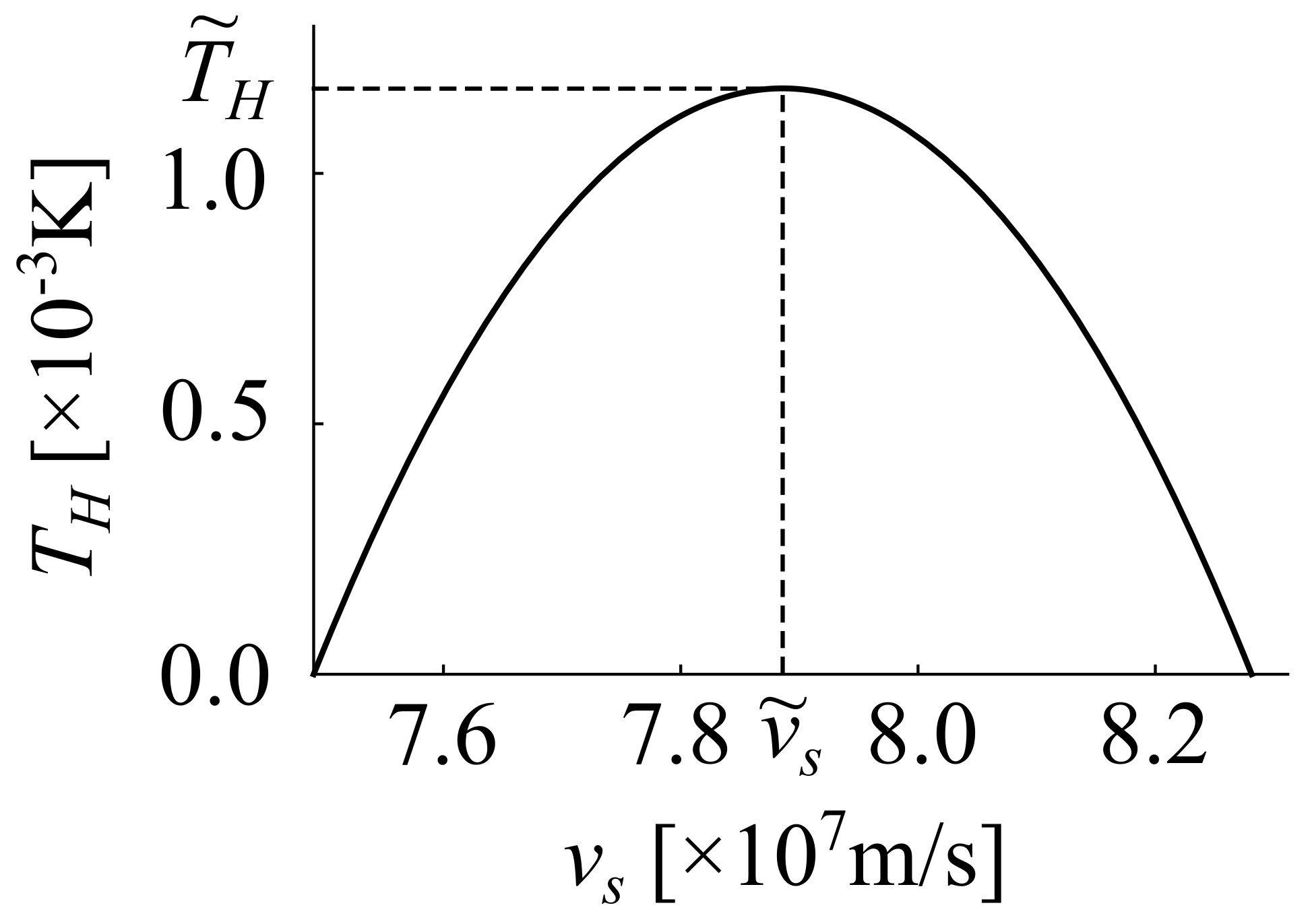
The Hawking temperature depends on the soliton velocity, as shown in Figure 6, and reaches the maximum where the gradient of the electromagnetic-wave velocity at the horizon is the largest. The soliton velocity , which gives the maximum Hawking temperature, is derived by
Solving this equation, we obtain
and
which means that the order of magnitude of the Hawking temperature is dominated by . The Hawking temperature reaches the milli-Kelvin order with experimentally feasible circuit parameters, as shown in Figure 6. This demonstrates that Hawking radiation is observable in our system.
4. Discussion
We have proposed the analogue black hole in LC transmission lines with nonlinear capacitors and shown that the voltage dark soliton obeying a nonlinear Schrödinger equation exists in the LC transmission lines by using discrete reductive perturbation methods. The voltage soliton can propagate through the transmission line without causing any unnecessary heat generation, and it spatially modifies the capacitance owing to the nonlinearity of the capacitor, leading to the spatial change of the electromagnetic-wave velocity in the transmission line. These spatial changes in the electromagnetic-wave velocity lead to the generation of the analogue black holes. This analogue black hole is dual to the one in Josephson transmission lines with nonlinear inductors [8], where the velocity of electromagnetic waves is spatially modulated through the nonlinear Josephson inductance.
We also evaluated the Hawking temperature using the conventional formula based on the gradient of surface gravity. Using the existing available circuit parameters, we found the Hawking temperature to be on the order of milli-Kelvin, by which we can conclude that Hawking radiation is observable in the transmission lines. We also identified the observed radiation as Hawking radiation by evaluating the soliton-velocity dependence of the Hawking temperature, as it depends on the soliton velocity.
We can extend our analogue black hole to the theory of black hole lasers in future work. There have been proposals of black hole lasers composed of two horizons behaving like a resonator for amplifying Hawking radiation [25,26,27,28,29]. However, as yet there has been no proposal of the black hole lasers in electric circuits. Two horizons need to be combined to produce the resonator. We believe that this can be achieved by pairing solitons and anti-solitons that correspond to black holes and white holes, respectively [10]. This will be discussed in our forthcoming paper.
Author Contributions
Conceptualization, H.K., N.H. and K.-i.M.; methodology, H.K., N.H. and K.-i.M.; software, H.K., N.H. and K.-i.M.; validation, H.K., N.H. and K.-i.M.; formal analysis, H.K., N.H. and K.-i.M.; investigation, H.K., N.H. and K.-i.M.; resources, H.K., N.H. and K.-i.M.; data curation, H.K., N.H. and K.-i.M.; writing—original draft preparation, H.K., N.H. and K.-i.M.; writing—review and editing, H.K., N.H. and K.-i.M.; visualization, H.K., N.H. and K.-i.M.; supervision, H.K., N.H. and K.-i.M.; project administration, H.K., N.H. and K.-i.M.; funding acquisition, H.K., N.H. and K.-i.M.. All authors have read and agreed to the published version of the manuscript.
Funding
This work was supported by JSPS KAKENHI Grant Number JP21J22333.
Institutional Review Board Statement
Not applicable.
Informed Consent Statement
Not applicable.
Data Availability Statement
Data available on reasonable request to the authors.
Acknowledgments
The authors thank T. Fujii for the insightful discussions.
Conflicts of Interest
The authors declare no conflict of interest.
Appendix A. Discrete Reductive Perturbation Method
Here we derive the nonlinear Schrödinger equation from circuit Equation (10) by using discrete reductive perturbation methods. We substitute Equations (12) and (14) into circuit Equation (10) and obtain the fundamental relations in our system for each order.
For the order, we obtain
This leads to the dispersion relation, as expressed in Equation (15).
For the order, the following relation holds:
This yields the group velocity, as expressed in Equation (30).
For the order, we satisfy
This results in our desired nonlinear evolution equation, the so-called nonlinear Schrödinger equation, Equation (18).
References
- Hawking, S.W. Particle creation by black holes. Commun. Math. Phys. 1975, 43, 199–220. [Google Scholar] [CrossRef]
- Unruh, W.G. Experimental Black-Hole Evaporation? Phys. Rev. Lett. 1981, 46, 1351–1353. [Google Scholar] [CrossRef]
- Jacobson, T.A.; Volovik, G.E. Event horizons and ergoregions in 3He. Phys. Rev. D 1998, 58, 064021. [Google Scholar] [CrossRef] [Green Version]
- Garay, L.J.; Anglin, J.R.; Cirac, J.I.; Zoller, P. Sonic Analog of Gravitational Black Holes in Bose-Einstein Condensates. Phys. Rev. Lett. 2000, 85, 4643–4647. [Google Scholar] [CrossRef] [Green Version]
- Philbin, T.G.; Kuklewicz, C.; Robertson, S.; Hill, S.; König, F.; Leonhardt, U. Fiber-Optical Analog of the Event Horizon. Science 2008, 319, 1367–1370. [Google Scholar] [CrossRef] [Green Version]
- Schützhold, R.; Unruh, W.G. Hawking Radiation in an Electromagnetic Waveguide? Phys. Rev. Lett. 2005, 95, 031301. [Google Scholar] [CrossRef] [Green Version]
- Nation, P.D.; Blencowe, M.P.; Rimberg, A.J.; Buks, E. Analogue Hawking Radiation in a dc-SQUID Array Transmission Line. Phys. Rev. Lett. 2009, 103, 087004. [Google Scholar] [CrossRef] [Green Version]
- Katayama, H.; Hatakenaka, N.; Fujii, T. Analogue Hawking radiation from black hole solitons in quantum Josephson transmission lines. Phys. Rev. D 2020, 102, 086018. [Google Scholar] [CrossRef]
- Katayama, H.; Ishizaka, S.; Hatakenaka, N.; Fujii, T. Solitonic black holes induced by magnetic solitons in a dc-SQUID array transmission line coupled with a magnetic chain. Phys. Rev. D 2021, 103, 066025. [Google Scholar] [CrossRef]
- Katayama, H. Designed Analogue Black Hole Solitons in Josephson Transmission Lines. IEEE Trans. Appl. Supercond. 2021, 31, 1–5. [Google Scholar] [CrossRef]
- Nation, P.D.; Johansson, J.R.; Blencowe, M.P.; Nori, F. Colloquium: Stimulating uncertainty: Amplifying the quantum vacuum with superconducting circuits. Rev. Mod. Phys. 2012, 84, 1–24. [Google Scholar] [CrossRef] [Green Version]
- Russell, J.S. Report on waves. In Proceedings of the the Fourteenth Meeting of the British Association for the Advancement of Science, York, UK, September 1844; pp. 311–390. [Google Scholar]
- Zabusky, N.J.; Kruskal, M.D. Interaction of “Solitons” in a Collisionless Plasma and the Recurrence of Initial States. Phys. Rev. Lett. 1965, 15, 240–243. [Google Scholar] [CrossRef] [Green Version]
- Gardner, C.S.; Greene, J.M.; Kruskal, M.D.; Miura, R.M. Method for Solving the Korteweg-deVries Equation. Phys. Rev. Lett. 1967, 19, 1095–1097. [Google Scholar] [CrossRef]
- Hasegawa, A.; Tappert, F. Transmission of stationary nonlinear optical pulses in dispersive dielectric fibers. I. Anomalous dispersion. Appl. Phys. Lett. 1973, 23, 142–144. [Google Scholar] [CrossRef]
- Toda, M. Vibration of a Chain with Nonlinear Interaction. J. Phys. Soc. Jpn. 1967, 22, 431–436. [Google Scholar] [CrossRef]
- Taniuti, T.; Yajima, N. Perturbation Method for a Nonlinear Wave Modulation. I. J. Math. Phys. 1969, 10, 1369–1372. [Google Scholar] [CrossRef]
- Kengne, E. and Bame, C. Dynamics of Modulated Wave Trains in a Discrete Nonlinear-dispersive Dissipative Bi-inductance Transmission Line. Czechoslov. J. Phys. 2005, 55, 609–630. [Google Scholar] [CrossRef]
- Kengne, E.; Lakhssassi, A. Analytical study of dynamics of matter-wave solitons in lossless nonlinear discrete bi-inductance transmission lines. Phys. Rev. E 2015, 91, 032907. [Google Scholar] [CrossRef]
- Kengne, E.; Lakhssassi, A. Analytical studies of soliton pulses along two-dimensional coupled nonlinear transmission lines. Chaos Solitons Fractals 2015, 73, 191–201. [Google Scholar] [CrossRef]
- Kengne, E.; Liu, W.M. Transmission of rogue wave signals through a modified Noguchi electrical transmission network. Phys. Rev. E 2019, 99, 062222. [Google Scholar] [CrossRef]
- Abdoulkary, S.; English, L.; Mohamadou, A. Envelope solitons in a left-handed nonlinear transmission line with Josephson junction. Chaos Solitons Fractals 2016, 85, 44–50. [Google Scholar] [CrossRef]
- Ghafouri-Shiraz, H.; Shum, P. Narrow pulse formation using nonlinear LC ladder networks. Fiber Integr. Opt. 1996, 15, 305–323. [Google Scholar] [CrossRef]
- Taniuti, T. Reductive Perturbation Method and Far Fields of Wave Equations. Prog. Theor. Phys. Suppl. 1974, 55, 1–35. [Google Scholar] [CrossRef] [Green Version]
- Corley, S.; Jacobson, T. Hawking spectrum and high frequency dispersion. Phys. Rev. D 1996, 54, 1568–1586. [Google Scholar] [CrossRef] [Green Version]
- Corley, S. Computing the spectrum of black hole radiation in the presence of high frequency dispersion: An analytical approach. Phys. Rev. D 1998, 57, 6280–6291. [Google Scholar] [CrossRef] [Green Version]
- Corley, S.; Jacobson, T. Black hole lasers. Phys. Rev. D 1999, 59, 124011. [Google Scholar] [CrossRef] [Green Version]
- Steinhauer, J. Observation of self-amplifying Hawking radiation in an analogue black-hole laser. Nat. Phys. 2014, 10, 864–869. [Google Scholar] [CrossRef]
- Gaona-Reyes, J.L.; Bermudez, D. The theory of optical black hole lasers. Ann. Phys. 2017, 380, 41–58. [Google Scholar] [CrossRef] [Green Version]
Figure 1.
Nonlinear LC transmission line consisting of constant inductance L and nonlinear capacitance depending on voltage . The unit cell length is denoted by a. The current and the voltage on the nth unit cell are and , respectively.
Figure 1.
Nonlinear LC transmission line consisting of constant inductance L and nonlinear capacitance depending on voltage . The unit cell length is denoted by a. The current and the voltage on the nth unit cell are and , respectively.
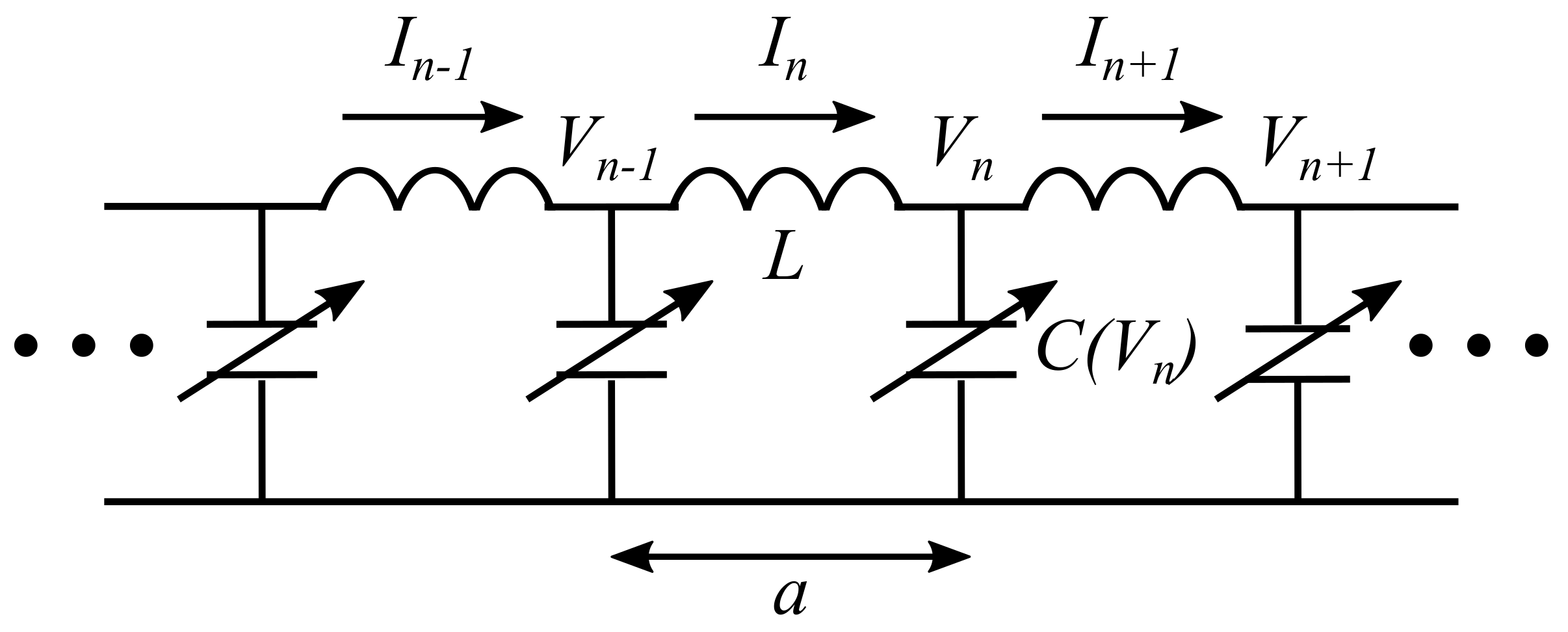
Figure 2.
Diagram of dispersion relation in our system. We set the circuit parameters to m, H, and F.
Figure 2.
Diagram of dispersion relation in our system. We set the circuit parameters to m, H, and F.
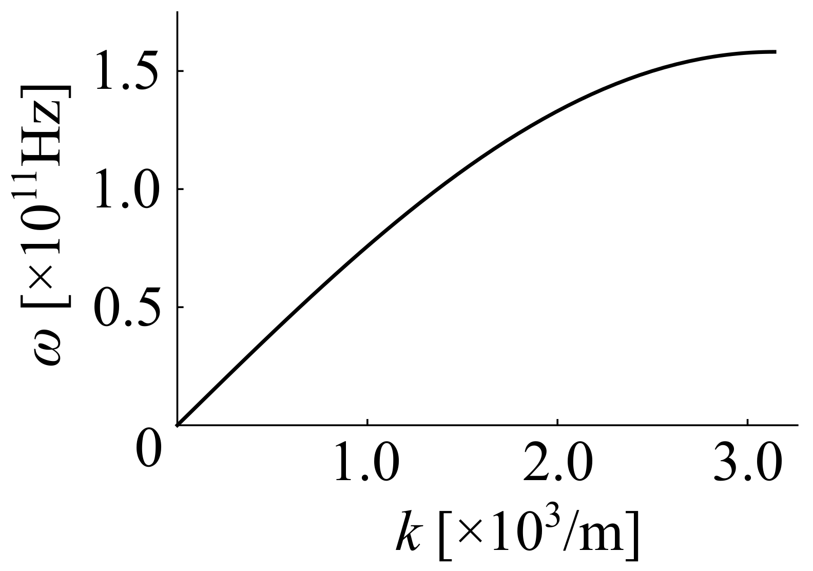
Figure 3.
Phase velocity (solid line) and group velocity (dashed line) as a function of wavenumber k. The circuit parameter values are the same as in Figure 2. The phase velocity is always larger than the group velocity.
Figure 3.
Phase velocity (solid line) and group velocity (dashed line) as a function of wavenumber k. The circuit parameter values are the same as in Figure 2. The phase velocity is always larger than the group velocity.
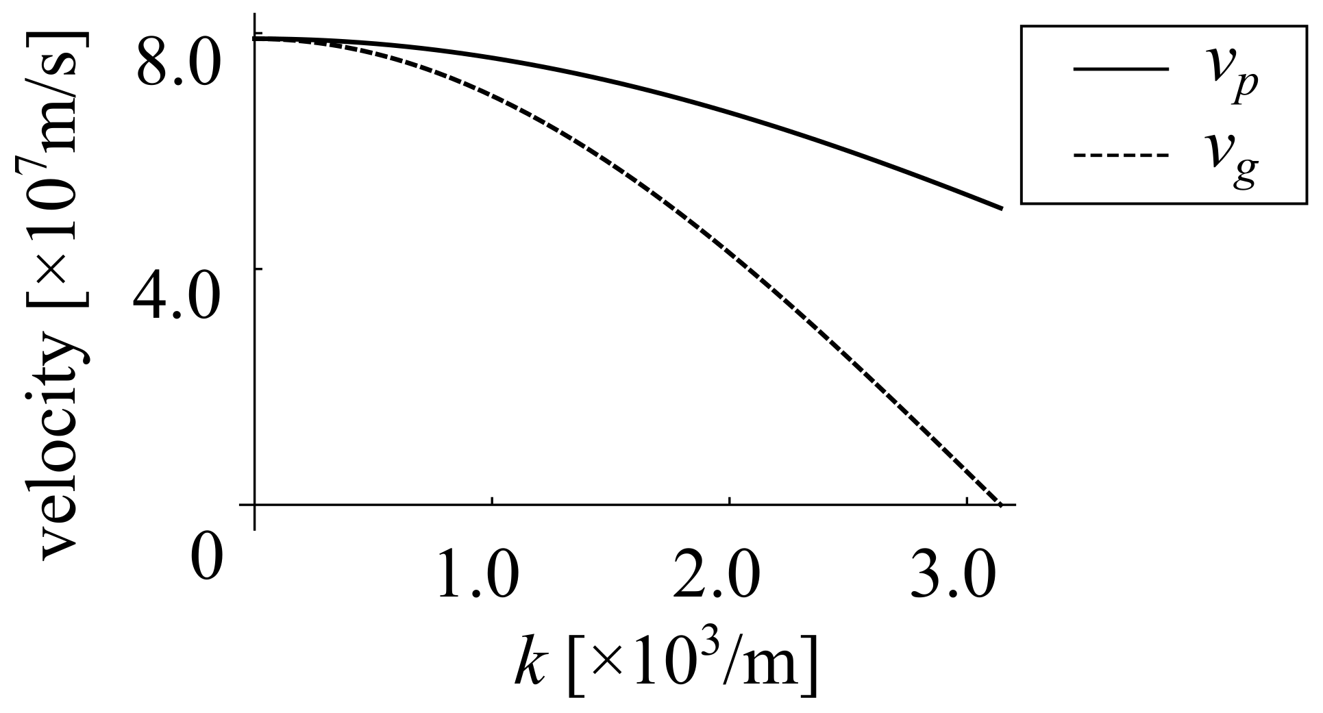
Figure 4.
Schematic diagram of (a) a bright soliton and (b) a dark soliton in co-moving frame described by Equations (22) and (23), respectively. The amplitude is represented by .

Figure 5.
(a) Schematic diagram of nonlinear transmission lines. (b) A voltage soliton in the co-moving frame . We set V and V, with the other circuit parameters the same as those in Figure 2. The soliton width is about . (c) The spatially varying group velocity of the electromagnetic waves in the co-moving frame for the wavenumber /m with the same circuit parameters. The horizontal dashed line represents the soliton velocity . The event horizon is formed at , where .
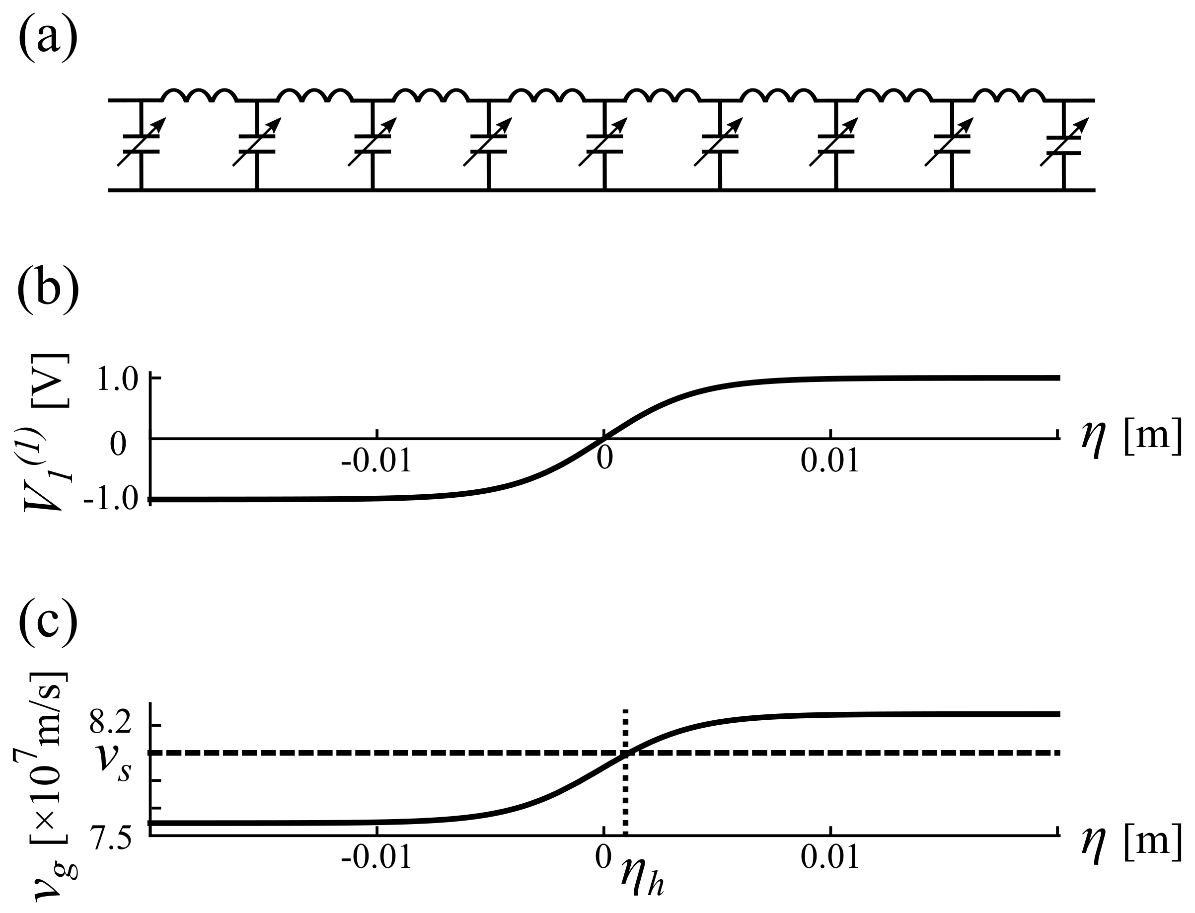
Figure 6.
Dependence of Hawking temperature on soliton velocity. The Hawking temperature reaches the maximum at the soliton velocity . The circuit parameters are the same as in Figure 5.
Figure 6.
Dependence of Hawking temperature on soliton velocity. The Hawking temperature reaches the maximum at the soliton velocity . The circuit parameters are the same as in Figure 5.
Publisher’s Note: MDPI stays neutral with regard to jurisdictional claims in published maps and institutional affiliations. |
© 2021 by the authors. Licensee MDPI, Basel, Switzerland. This article is an open access article distributed under the terms and conditions of the Creative Commons Attribution (CC BY) license (https://creativecommons.org/licenses/by/4.0/).
Share and Cite
MDPI and ACS Style
Katayama, H.; Hatakenaka, N.; Matsuda, K.-i. Analogue Hawking Radiation in Nonlinear LC Transmission Lines. Universe 2021, 7, 334. https://doi.org/10.3390/universe7090334
AMA Style
Katayama H, Hatakenaka N, Matsuda K-i. Analogue Hawking Radiation in Nonlinear LC Transmission Lines. Universe. 2021; 7(9):334. https://doi.org/10.3390/universe7090334
Chicago/Turabian StyleKatayama, Haruna, Noriyuki Hatakenaka, and Ken-ichi Matsuda. 2021. "Analogue Hawking Radiation in Nonlinear LC Transmission Lines" Universe 7, no. 9: 334. https://doi.org/10.3390/universe7090334
Note that from the first issue of 2016, this journal uses article numbers instead of page numbers. See further details here.