Article

Constraints on Dark Energy Models from Galaxy Clusters and Gravitational Lensing Data

by
Alexander Bonilla
1,2,* and
Jairo E. Castillo
2
1
Departamento de Física, Universidade Federal de Juiz de Fora, 36036-330 Juiz de Fora, MG, Brazil
2
Grupo de Investigación en Física, Matemáticas y Computación, Línea de Cosmología y Astrofísica, Facultad Tecnológica, Unversidad Distrital Francisco José de Caldas, Carrera 7 No. 40B-53, Bogotá, Colombia
*
Author to whom correspondence should be addressed.
Universe 2018, 4(1), 21; https://doi.org/10.3390/universe4010021
Submission received: 19 September 2017 / Revised: 8 January 2018 / Accepted: 9 January 2018 / Published: 22 January 2018
(This article belongs to the Special Issue Progress in Cosmology in the Centenary of the 1917 Einstein Paper)

Abstract

:
The Sunyaev–Zel’dovich (SZ) effect is a global distortion of the Cosmic Microwave Background (CMB) spectrum as a result of its interaction with a hot electron plasma in the intracluster medium of large structures gravitationally viralized such as galaxy clusters (GC). Furthermore, this hot gas of electrons emits X-rays due to its fall in the gravitational potential well of the GC. The analysis of SZ and X-ray data provides a method for calculating distances to GC at high redshifts. On the other hand, many galaxies and GC produce a Strong Gravitational Lens (SGL) effect, which has become a useful astrophysical tool for cosmology. We use these cosmological tests in addition to more traditional ones to constrain some alternative dark energy (DE) models, including the study of the history of cosmological expansion through the cosmographic parameters. Using Akaike and Bayesian Information Criterion, we find that the w C D M and Λ C D M models are the most favoured by the observational data. In addition, we found at low redshift a peculiar behavior of slowdown of the universe, which occurs in dynamical DE models when we use data from GC.

1. Introduction

Several authors have used the Sunyaev–Zel’dovich (SZ) effect, X-rays and Strong Gravitational Lens (SGL) data from galaxies and galaxy clusters (GC) to provide independent estimations of cosmological parameters. The combination of X-rays and the SZ data leads to two useful cosmological tests, namely angular diameter distance d A [1] and gas mass fraction f g a s of the GC [2]. Both tests have been used in the literature to investigate dark energy (DE) [3] and modified gravity (see [4] and reference therein). Additionally, the SGL observations also can be used to probe the dark matter (DM) and DE properties [3]. Therefore, to use the GC measures constitutes an independent and complementary test to probe cosmological models. Now, from the phenomenological point of view, the Λ C D M (Cosmological constant + Cold Dark Matter) model is the most accepted to date, which predicts that the universe consists of approximately 4 % of baryonic matter, 26 % of CDM and about 70 % is a exotic component known as DE, which is mainly responsible for the accelerated expansion of the Universe nowadays. In the concordance model ( Λ C D M ), it is assumed that CDM is made up of collisionless non baryonic particles and DE is driven by cosmological constant Λ , which has an equation of state (EoS) w = 1 . From this perspective, the concordance model is in excellent agreement with the observations of Supernova Ia (SNIa), cosmic microwave background (CMB) anisotropies and baryonic acoustic oscillations (BAO). However, Λ C D M model has some unresolved fundamental issues about the nature of the of DM and DE [5,6]. With respect to DE, there are different theoretical arguments against Λ . The first is the coincidence problem, which establishes the question of: why do the values of DE and DM density have the same order of magnitude today? Another important issue is related to “fine tuning” of the value of the cosmological constant to the present, which is in complete disagreement with quantum field theory and particle physics [7,8]. In this way, several DE models with a dynamical EoS have been proposed to try to solve the so-called “cosmological constant problem” [6,8].
Our main aim in this paper is to impose the constraints on some well established cosmological models in the literature with the use of GC and SGL in the frame of Friedmann–Lemaître–Robertson– Walker (FLRW) cosmology.
This paper is organized as follows. In Section 2, we introduce the cosmological tests and the statistical analysis. In Section 3, we describe cosmological models of DE, including the main results. The history of expansion is analyzed in Section 4. In Section 5, we provide the summary and the discussion.

2. Galaxy Clusters

The GC are the biggest gravitational structures in the Universe. They are in the transition between the linear and nonlinear regimes of the structure formation. Gravitational lensing of background sources produced by these systems are used to infer the shape of matter distributions in the Universe. Nevertheless, some lensing results such as high Navarro–Frenk–White concentration parameters and the predictions of the Einstein radii distributions are in tension with the standard Λ CDM model [9]. Therefore, the study of GC is very important for cosmology because it offers information that can be used to develop cosmological tests that help to distinguish between different models of DE present in the literature. In what follows, we describe briefly three different data sets that will be used in the development of these cosmological tests: the GC (SZ/X-ray, f g a s ) and SGL.

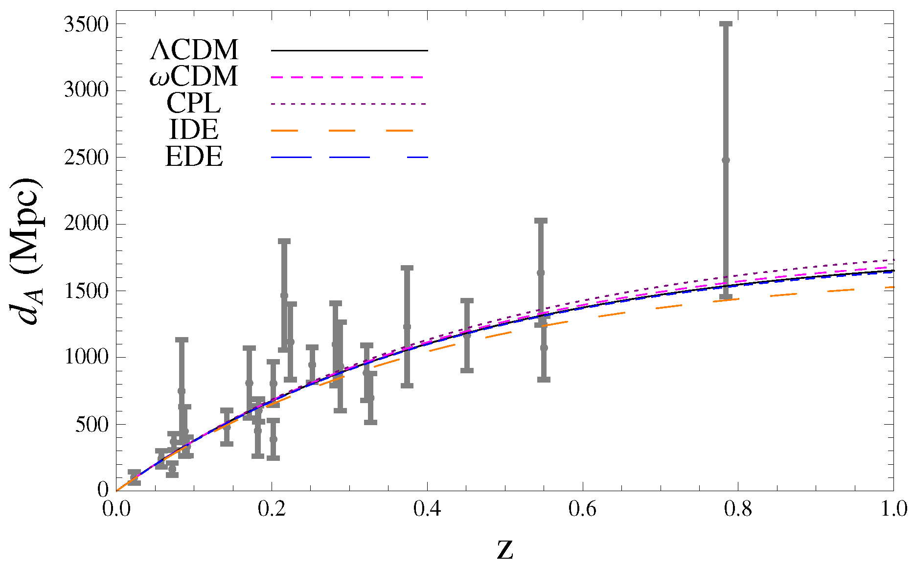
2.1. Angular Diameter Distance Using the SZ/X-Ray Method

The thermal SZ effect is a small distortion in cosmic microwave background (CMB) spectrum due to the inverse Compton scattering of the CMB photons when they pass through the hot gas of electrons in GC [10,11]. This small fluctuation in CMB temperature is characterized by Δ T s z / T c m b = f ( ν , T e ) y ( n e , T e ) , where
y ( n e , T e ) = l o s n e k B T e m e c 2 σ T d l ,
which is known as the Compton parameter, such that T c m b = 2.726 K, n e and T e are the temperature of CMB, electron number density and temperature of the hot gas, respectively. σ T is the Thomson cross section, k B is the Boltzmann constant, m e c 2 is the rest mass of the electron and the integration is along the line of sight (los). The dependence with the frequency of the thermal SZ effect is given through the term f ( ν , T e ) , which also introduces relativistic corrections (see [12] for more details and [13] for a more recent update).
On the other hand, gas in GC can reach temperatures of 10 7 10 8 K and densities of the order of 10 1 10 5 cm 3 , so they emit high amounts of energy in X-rays. The primary emission mechanisms of X-rays for a diffuse intra-cluster medium are collisional processes such as: free–free (Bremsstrahlung), free–bound (recombination) or bound–bound (mainly emission lines), with luminosities of the order of 10 44 erg/s or even higher and spatial extensions of several arcmin or larger, even at high redshift. X-rays’ observations currently offer a powerful technique for building catalogs of galaxy clusters, which are very important for modern cosmology [14]. The X-ray GC emission is given by
S x = 1 4 π ( 1 + z ) 4 n e 2 Λ e H ( μ e / μ H ) d l ,
where Λ e H is the X-ray cooling function, μ is the molecular weight given by μ i = ρ / ( n i m p ) and z is the cluster redshift [1,2]. Then, combining Equations (1) and (2) through n e , we can obtain experimental cosmological distance with triaxial symmetry, given by
D c | e x p e l l = Δ T S Z 0 2 S x 0 m e c 2 k B T e 2 g ( β ) g ( β / 2 ) 2 θ c , p r o j Λ e H ( μ e / μ H ) 4 π 3 / 2 f ( ν , T e ) 2 T c m b 2 σ T 2 ( 1 + z ) 4 ,
where Δ T S Z 0 and S x 0 are the central temperature decrement and the central surface brightness, respectively, which include all the physical constants and the terms resulting from the los integration, such that Δ T S Z 0 d A ( z ) , S x 0 d A ( x ) and d A ( z ) = D c | e x p e l l h 3 / 4 ( e p r o j / e 1 e 2 ) 1 / 2 , h is a function of GC shape and orientation, e p r o j is axial ratio of the major to minor axes of the observed projected isophotes and θ c , p r o j is the projection on the plane of the sky (pos) (see Appendix A for some useful relationships and Table A1 for some data used in these methods). The expression in Equation (3) is an observational quantity that depends basically on the physical and geometrical properties of the cluster (see [1] for more information about the astrophysical details). That method for measuring distances is completely independent of other techniques and is valid at any redshift. We use 25 measurements of angular diameter distances from GC obtained through SZ/X-ray method by De Filippis et al. (see Figure A2). In our analysis, we follow the standard procedure and minimize the χ 2 function
χ d i s 2 ( z i , Θ ) = i = 1 25 D c | e x p e l l ( z i ) d A ( z ) 2 σ D c 2 ,
where d A ( z ) is the angular diameter distance in a FLRW universe and σ D c 2 are the errors associated with D c | e x p e l l ( z i ) (see Table A1 in Appendix).

2.2. The Gas Mass Fraction f g a s

Another independent cosmological technique is to derive d A using the gas mass fraction data from GC. In order to use f g a s as a cosmological test, we need to assume that there is a proportion between the baryonic fraction of the GC and the global fraction of baryonic matter and DM. Moreover, it is necessary to assume that the baryonic fraction from clusters does not depend on the redshift [15]. This assumption is valid if one considers that these clusters are formed approximately by the same time.1 (see [16] for more details). Thus, the gas mass fraction can be defined as f g a s M g a s / M t o t , where M g a s is the X-ray’s gas mass and M t o t is the total gravitational mass of GC respectively. To relate f g a s with the parameters of a particular cosmological model, we can write M g a s and M t o t in terms of d A ( z ) as follows [17],
f g a s Λ C D M ( z ) b 1 + α Ω b Ω 0 m d A Λ C D M ( z ) d A ( z ) 3 / 2 ,
where d A ( z ) is the angular diameter distance for a given cosmological model and d A Λ C D M ( z ) is the angular diameter distance for a reference model; in this case, let us assume the Λ C D M model. Here, Ω b and Ω 0 m are the baryonic density parameter and the DM density parameter, respectively. The parameter b is the depletion factor that relates the baryonic fraction in clusters to the mean cosmic value. The constant α is the ratio between optically luminous baryonic mass in galaxies (stellar mass) to the baryonic X-ray gas mass in intracluster medium, and its value is given by α 0.19 h [16]. The factor h is the normalized Hubble constant, that is, h = H 0 / 100 km s 1 Mpc 1 . Let us use the f g a s measurements from 42 GC obtained in [18]. The χ 2 is defined as
χ f g a s 2 ( z i , Θ ) = i = 1 42 [ f g a s Λ C D M ( z i , Θ ) f g a s ( z i , Θ ) ] 2 σ f g a s 2 + Ω b h 2 0.0214 0.0020 2 + h 0.72 0.08 2 + b 0.824 0.089 2 ,
where f g a s is observational gas mass fraction data [18] and σ f g a s are the systematic errors. In the analysis, we have considered b = 0.824 [16].

2.3. Gravitational Lensing

The gravitational lens effect is one of the queen’s tests of General Relativity. Strong gravitational lensing occurs when the light rays of a source are strongly deflected by the lens producing multiples images. The position of these images depend on the properties of the lens mass distribution [19]. Because the Einstein radii, θ E , also depends on a cosmological model, the SL observations can be used as an additional method to probe the nature of the DE [3,20]. In this work, we use the method that consists of comparing the ratio D of angular diameter distances between lens and source, d A ( z l , z s ) , and between observer and lens, d A ( 0 , z s ) , with its observable counterpart D o b s given by
D ( z l , z s ) = d A ( z l , z s ) d A ( 0 , z s ) = z l z s d z / E ( z , Θ ) 0 z s d z / E ( z , Θ ) ,
D o b s = c 2 θ E 4 π σ S I S 2 ,
where σ S I S is the Singular Isothermal Sphere (SIS) velocity dispersion and E ( z , Θ ) H ( z , Θ ) / H 0 , H ( z , Θ ) being the Hubble function. In order to put constraints on cosmological parameters through E ( z , Θ ) , the Einstein radius θ E and the dispersion velocity σ S I S (exactly its central velocity dispersion σ 0 ) must be obtained by astrometric and spectroscopic means, respectively. In the first case, it depends on the lens modelling (either SIS, Singular Isothermal Ellipsoid (SIE) or Navarro–Frenk–White density profiles). In the second case, the velocity dispersion σ S I S of the mass distribution and the observed stellar velocity dispersion σ 0 need not be the same, since the halos of DM can have a greater speed of dispersion than the visible stars [21]. These effects can be taken into account through the following relationship σ S I S = f E σ 0 , where the parameter f E emulates the systematic errors in the RMS due to the difference between σ S I S and σ 0 ; the rms error caused by assuming the SIS model, since the observed image separation does not directly correspond to θ E and softened SIS potentials which tend to decrease the typical image separations [22]. In the present work we assume the best-fit reported in [20] (and references therein), where f E 1 , which has been properly marginalized. On the other hand, GC can also act as sources to produce strong gravitational lensing showing giant arcs around GC. This phenomenon can be used to constrain the astrophysical properties of the cluster (projected mass) and cosmology [23]. If we assume the condition of hydrostatic equilibrium 2 and an approximation of spherical symmetry 3 [24], then a theoretical surface density can be described as
Σ t h = 3 2 G μ m p k B T X β X d A ( 0 , z l ) θ c ,
where k B , m p , μ = 0.6 and β X are, respectively, the Boltzmann constant, the proton mass, the mean molecular weight and the slope of the β m o d e l [25]. Although the hydrostatic equilibrium and isothermal hypotheses are very strong, the total mass density obtained under such assumption may lead to good estimates, even in dynamically active GC with irregular morphologies in X-rays. Then, combining this with the critical surface mass density for lensing Σ o b s [26], We can get a Hubble constant independent ratio as
D o b s = d A ( z l , z s ) d A ( 0 , z s ) = μ m p c 2 6 π 1 k B T X β X θ t 2 + θ c 2 ,
where the parameters T X , β X and θ c can be obtained from X-ray observational data. The position of tangential critical curve θ t = ϵ θ a r c , where θ a r c is the observational arc position and ϵ = ( 1 / 1.2 ) ± 0.04 quantifies the slight difference with arc radius angle (See [27,28] for more details about the priors and 10 galaxy clusters used as sample).
In the present work we use a sample of 80 strong lensing systems by [20], which contains 70 data points from SLACS and LSD and 10 data points from GC. Again, the fit of the theoretical models to strong lensing observations can be found by the minimization of
χ S L 2 = i = 1 80 D i o b s D i t h 2 σ D , i 2 ,
where the sum is over the sample and σ D , i 2 denotes the variance of D i o b s .
Additionally to these data sets defined in the Section 2.1, Section 2.2 and Section 2.3, we will use 580 Supernovae data (SNIa) from Union 2.1 [29], the CMB shift parameter [30] (Planck 2013), as well as data from BAO (BOSS, WiggleZ, SDSS, 6dFGS) observations, adopting the three measurements of A ( z ) obtained from [31,32], and using the covariance among these data given in [33]. Each χ 2 function is constructed in a way analogous to the other tests considered above (see Appendix B).

2.4. Statistic Analysis

The procedure of finding a set of parameters for a given statistic is known as Maximum likelihood L m a x , that is, given a probability distribution this is maximum for the corresponding data set. The maximum likelihood estimate for the best fit parameters p i m is given by
L m a x ( p i m ) = e x p 1 2 χ m i n 2 ( p i m ) .
If L m a x ( p i m ) has a Gaussian errors distribution, then χ m i n 2 ( p i m ) = 2 ln L m a x ( p i m ) , which is our case [34]. In order to find the best values of the free parameters of the model, let us consider
χ t o t a l 2 = χ S N I a 2 + χ C M B 2 + χ B A O 2 + χ d A 2 + χ f g a s 2 + χ S G L 2 .
The Fisher matrix is used in the analysis of the constraint of cosmological models for different observational test [35,36]. It contains the Gaussian uncertainties σ i 2 of the different parameters p i m . Given the best fit χ m i n 2 ( p i m , σ i 2 ) for a set of parameters p i m with uncertainties σ i 2 , the Fisher matrix is
F i j = 1 2 2 χ m i n 2 p i m p j m
for each model m. The inverse of the Fisher matrix provides an estimate of the covariance matrix through C c o v = F 1 . Its diagonal elements are the squares of the uncertainties in each parameter marginalizing over the others, while the off-diagonal terms yield the correlation coefficients between parameters. The uncertainties obtained in the propagation of errors are given by σ i = D i a g C c o v i j . Notice that the marginalized uncertainty is always greater than (or at most equal to) the non-marginalized one: marginalization can’t decrease the error, and only has no effect if all other parameters are uncorrelated with it 4. Previously known uncertainties on the parameters, known as priors, can be trivially added to the calculated Fisher matrix. This is manifestly the case for us: a lot of standard cosmological datasets provide priors on our previously defined cosmological parameters. The analysis with the Fisher matrix is used to evaluate the errors on the best-fit parameters.
In our results, let us consider different cosmological models. Thus, a way to quantify which model best fit the data is consider a Bayesian comparison. We adopted the Akaike and Bayesian information criterion (AIC and BIC, respectively), which allows us to compare cosmological models with different degrees of freedom, with respect to the observational evidence and the set of parameters [37,38]. The AIC and BIC can be calculated as
A I C = 2 ln L m a x + 2 d ,
B I C = 2 ln L m a x + d ln N ,
where L m a x is the maximum likelihood of the model under consideration ( L m a x = e x p 1 2 χ m i n 2 ), d is the number of parameters and N the number of data points. The BIC imposes a strict penalty against extra parameters for any set with N data. The prefered model is that which minimizes the AIC and BIC. However, the absolute values of them are not of interest, only the relative values between the different models [39]. Therefore, the “strength of evidence” can be characterized in the form Δ A I C = A I C i A I C m i n , Δ B I C = B I C i B I C m i n , where the subindex i refers to value of A I C ( B I C ) for model i and A I C m i n ( B I C m i n ) is the minimum value of A I C ( B I C ) among all the models [40]. We give the judgements for both critera as follows: (i) If Δ A I C ( Δ B I C ) 2 , then the concerned model has substantial support with respect to the reference model (i.e., it has evidence to be a good cosmological model), (ii) if 4 Δ A I C ( Δ B I C ) 7 , it is an indication for less support with respect to the reference model, and, finally, (iii) if Δ A I C ( Δ B I C ) 10 , then the model has no observational support. Thus, if we have a set of models of DE, first we should estimate the best fit χ 2 and then we can apply the A I C and B I C to identify which model is the preferred one by the observations. We also apply the reduced chi-square to see how well the model fit the data, which is defined as χ r e d 2 = χ m i n 2 / ν , where ν is the degrees of freedom usually given by N d . Then, the total number of data points is: SNIa (580), CMB (3), BAO (7), d A (25), f g a s (42), SGL (80), so N = 737. Priors used in the present analysis are standard and the most conservative possible and combining GC data with independent constraints from CMB, BAO and SNIa removes the need of priors for Ω b , and h leads to tighter constraints over Ω m , Ω k and the parameters that characterize the DE density for different cosmological models. On the other hand, SGL offers a great opportunity to constrain DE features without prior assumptions on the fiducial cosmology. In what follows, we present our main results.

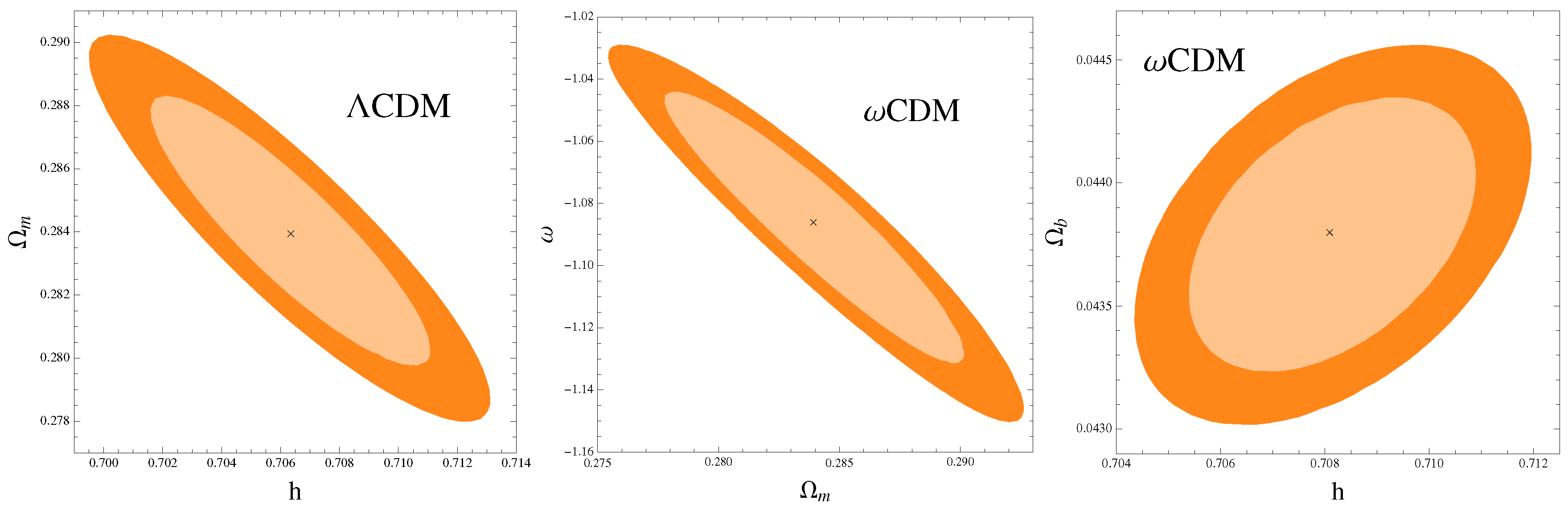
3. Dark Energy Models and Results

In order to put constraints on DE models using GC ( d A , f g a s ) and SGL, we need to compute the angular diameter distance of the model and compare it with observational data. In addition, to investigate whether a cosmological model can predict an accelerated expansion phase of the Universe, we must study the behavior of the deceleration parameter q ( z ) . The angular diameter distance for a FLRW universe, from a source at redshift z, is given by
d A ( z , Θ ) = 3000 h 1 ( 1 + z ) 1 Ω k sin ς 0 z Ω k E ( z , Θ ) d z ,
where h is dimensionless Hubble parameter ( H 0 = h 100 km s 1 Mpc 1 ) and the function sin ς ( x ) is defined such that it can be sinh ( x ) for Ω k > 0 , sin ( x ) for Ω k < 0 and x for Ω k = 0 [41]. In the standard FLRW cosmology, the expansion rate as a function of the scale factor H ( a ) is given by the Friedmann equation as
E 2 ( a , Ω i ) = Ω r a 4 + Ω m a 3 + Ω k a 2 + Ω X e 3 a 1 d a a 1 + w ( a ) ,
where H ( a ) / H 0 = E ( a , Ω i ) , H 0 is the current value of the expansion rate and the scale factor is related to redshift as 1 + z = a 1 , such that a 0 = 1 at present. In Equation (18), Ω i is a dimensionless energy densities relative to critical ( ρ c r i = 3 H 0 2 / 8 π G ) in the form of the ith component of the fluid density of: radiation ( Ω r ), matter ( Ω m ), curvature ( Ω k ) and DE ( Ω X ). Ω r 0 ( h ) = Ω γ ( h ) ( 1 + 0.2271 N e f f ) , where Ω γ ( h ) = 2.469 × 10 5 h 2 is the density of photons and N e f f = 3.046 is the effective number of neutrino species [42]. ω ( a ) = p ( a ) / ρ ( a ) is the EoS for DE, where p ( a ) is the fluid pressure. This EoS divides our models into two cases: when the energy density of the fluid is constant and the energy density of the fluid is dynamic. In all cosmological models, Ω k is a free parameter. A vector of parameters is considered for each DE model as Θ i m o d e l = θ i , Ω i , where θ i = h , Ω b for the analysis of the present work.

3.1. Λ C D M

Our analysis starts with standard cosmological model, where DE density is provided by the cosmological constant Λ . The expansion rate within Λ C D M context is given by
E 2 ( z , Θ ) = Ω r ( 1 + z ) 4 + Ω m ( 1 + z ) 3 + Ω k ( 1 + z ) 2 + Ω Λ ,
where Ω r , Ω m and Ω Λ = 1 Ω m Ω k Ω r , are the density parameters for radiation, matter and DE component, respectively. Here, the free parameter vector is Θ = h , Ω b , Ω m , Ω k . We find the best fit of parameters at 1 σ confidence level (CL), whose results are shown in Table 1.
In Table 1, we can see the impact of adding the GC and SGL tests to the more traditional ones (CMB + BAO + SNIa), which evidently improves the constraints on the parameters of the model (see Figure 1).

3.2. w C D M Model

The most simple extension of the Λ C D M model is to consider that the EoS remains constant but its value can be w 1 . In this case, the expansion rate for FLRW cosmology reads as
E 2 ( z , Θ ) = Ω r ( 1 + z ) 4 + Ω m ( 1 + z ) 3 + Ω k ( 1 + z ) 2 + Ω X ( 1 + z ) 3 ( 1 + w ) ,
where Ω X = ( 1 Ω m Ω k Ω r ) . In this model, the set of free parameters is Θ = h , Ω b , Ω k , Ω m , w . As in the case of Λ CDM model, first we estimate the best fit values using the data from S N I a + C M B + B A O and then, we use the full data set S N I a + C M B + B A O + d A + f g a s + S G L . The best fit values at 1 σ CL for this case is shown in the Table 2.
Notice that in both cases the EoS has a phantom behavior and the standard model is excluded at least up to 2 σ CL (see Figure 1). As the case of Λ CDM model, the curvature parameter changes from negative to positive (Table 2).

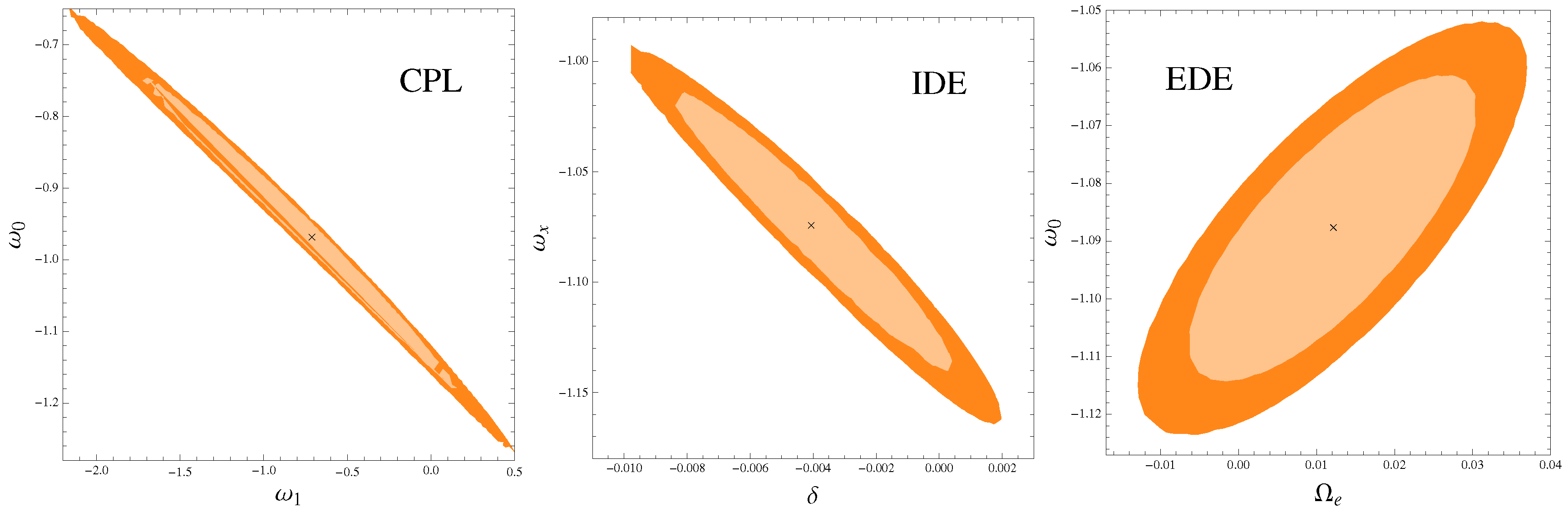
3.3. Chevalier–Polarski–Linder Model

Another simple extension to the Λ C D M model is to allow for the EoS of the DE varies with the redshift. Several parameterizations have been considered in the literature. Here, let us consider the popular Chevallier–Polarski–Linder (CPL) model [43,44]
w ( z ) = w 0 + w 1 z 1 + z ,
where w 0 is the value of the DE state equation at the present and the parameter w 1 evaluates the dynamic character of DE. The FLRW E ( z ) for CPL parametrization is given by
E 2 ( z ) = Ω r ( 1 + z ) 4 + Ω k ( 1 + z ) 2 + Ω m ( 1 + z ) 3 + Ω X X ( z ) ,
where Ω X = 1 Ω k Ω m Ω r and
X ( z ) = ( 1 + z ) 3 ( 1 + w 0 + w 1 ) exp 3 w 1 z 1 + z .
The free parameters are Θ = h , Ω b , Ω k , Ω m , w 0 , w 1 . The best fit values at 1 σ CL using C M B + B A O + S N I a and full data set are summarized in Table 3.
We can see that, for both the combined analyses, the CPL model allows a quintessential DE at the current time. The curvature parameter Ω k remains negative. The standard model remains within the 1 σ and 2 σ of CL for the present analysis (see Figure 1).

3.4. Interacting Dark Energy Model

Cosmological models, where DM and DE are non minimally coupled throughout the evolution history of the universe, have been considered to solve the problem of the cosmic coincidence as well as the problem of the cosmological constant (models where DM interacts with vacuum energy or Interacting Dark Energy (IDE) Models—see [45,46] for general review). It has recently been shown that the current observational data can favor the late-time interaction in the dark sector [47,48,49,50,51,52]. In general, we assume that DM and DE interact via a coupling function Q given by
ρ m ˙ + 3 H ρ m = Q ρ m , ρ x ˙ + 3 H 1 + w x ρ x = Q ρ m ,
where ρ m and ρ x are the DM and DE density, respectively, with w x the EoS for DE. Here, Q = δ H characterizes the strength of the interacting through the dimensionless coupling term δ , which establishes a transfer of energy from DE to DM for δ > 0 , whereas for δ < 0 the energy transfer is the opposite. This model was originally introduced in [53], and then investigated in various contexts [54,55,56]. The expansion rate of the Universe for this model is given by
E 2 ( z , Θ ) = Ω r ( 1 + z ) 4 + Ω k ( 1 + z ) 2 + Ω m Ψ ( z ) + Ω X ( 1 + z ) 3 ( 1 + w x ) ,
where Ω X = ( 1 Ω m Ω k Ω r ) and
Ψ ( z ) = δ ( 1 + z ) 3 ( 1 + w x ) + 3 w x ( 1 + z ) 3 δ δ + 3 w x .
This model is characterized by the following set of parameters Θ = h , Ω b , Ω k , Ω m , w x , δ . We show the best fit values of these parameters in Table 4.
Is interesting to note that, in both cases, EoS has a phantom behavior at present and the standard model is practically discarded at 1 σ CL. The curvature parameter Ω k is positive. We can also notice that the case δ = 0 (absence of interaction) is excluded at least to 2 σ CL for the present analysis, where we can appreciate that for both data sets the transfer of energy is from DM to DE (see see Figure 1).

3.5. Early Dark Energy Model

In early dark energy (EDE) scenarios, the DE density can be significant at high redshifts. This may be so if DE fluid tracks the dynamics of the background fluid density [57]. Here, we present the EDE model proposed by [58]. The FLRW equation for this model is
E 2 ( z , Θ ) = Ω r ( 1 + z ) 4 + Ω m ( 1 + z ) 3 + Ω k ( 1 + z ) 2 1 Ω X ,
where Ω X is given by
Ω X = Ω X 0 Ω e 1 ( 1 + z ) 3 w 0 Ω X 0 + f ( z ) + Ω e 1 ( 1 + z ) 3 w 0
and
f ( z ) = Ω m ( 1 + z ) 3 w 0 + Ω r ( 1 + z ) 3 w 0 + 1 + Ω k ( 1 + z ) 3 w 0 1 ,
such that Ω X 0 = 1 Ω m Ω k Ω r is the current DE density, Ω e is the asymptotic early DE density and w 0 is the present DE EoE. Here, we have six free parameters Θ = h , Ω b , Ω k , Ω m , Ω e , w 0 . The best fit values of the model parameters are summarized in Table 5.
For this model, the EoS keeps a phantom behavior at the present time and the standard model is discarded at least to 2 σ CL (see see Figure 1). Ω k is positive in both cases.

3.6. Statistical Discrimination Models

In Table 6, we present the values for the analysis of the information criterion with respect to the five cosmological models presented above, for used data set, namely CMB + BAO + SNIa + d A + f g a s s + SGL. As we can see, Δ A I C and Δ B I C are in favor of ω C D M and Λ C D M , respectively (approximately or less than two), and, hence, these models are in very good agreement with observations, which is also true for CPL, IDE and EDE models only with respect to Δ A I C . For models CPL, IDE and EDE, the value of Δ B I C is approximately equal to seven and therefore, according to this criterion, present less observational support.

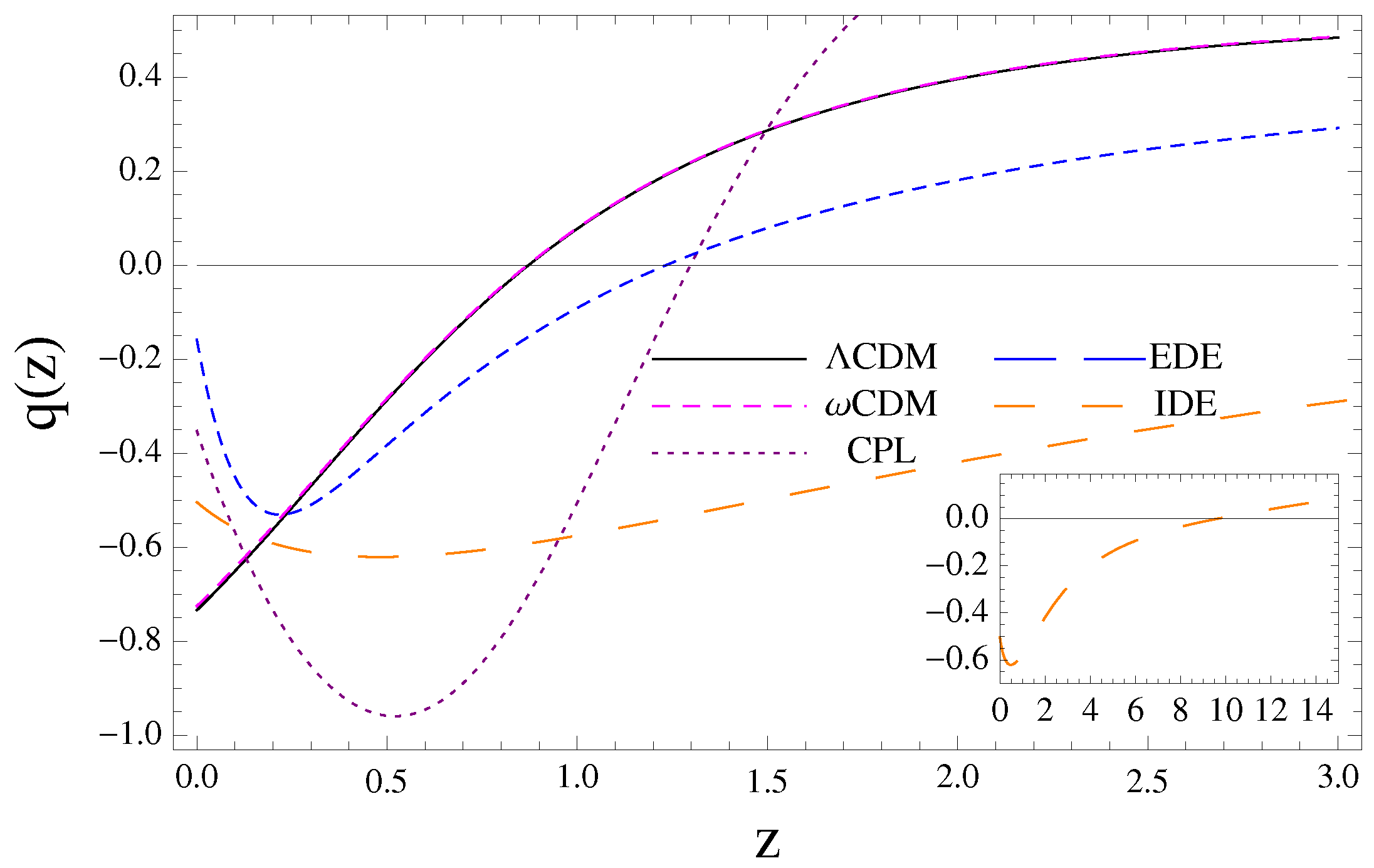
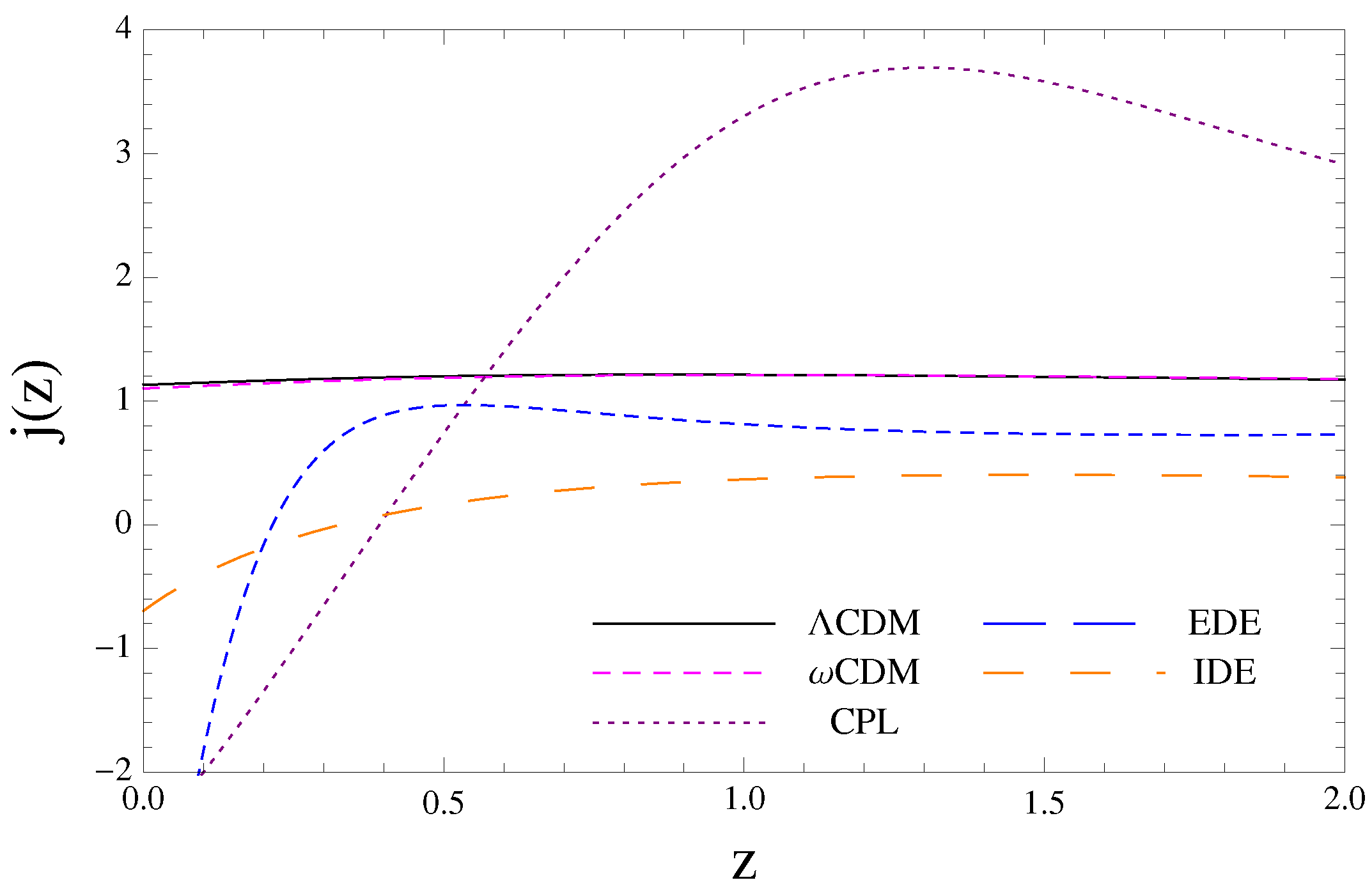
4. History of the Expansion and Cosmography

The kinematics of the universe can be described through the Hubble parameter H ( t ) and its dependence on time, i.e., the deceleration parameter q ( t ) [59] . Following [60], the scale factor a ( t ) can be expanded in Taylor series around the current time ( t 0 ) as:
a ( t ) a ( t 0 ) = 1 + H 0 1 ! t t 0 q 0 2 ! H 0 2 t t 0 2 + j 0 3 ! H 0 3 t t 0 3 + ,
where in general we can have a kinematic description of the cosmic expansion through the set of parameters:
H ( t ) 1 a d a d t ; q ( t ) 1 a d 2 a d t 2 H ( t ) 2 ; j ( t ) 1 a d 3 a d t 3 H ( t ) 3 ,
where the last term is know as jerk parameter j(t). The great advantage of this method is that we can investigate the cosmic acceleration without assuming any modification of gravity theory or DE model, due mainly to its geometric approximation. Although more terms of the series can be analyzed, we are only interested in the first three terms for the present work. The deceleration and jerk parameter are obtained as
q ( z ) = 1 + ( 1 + z ) H ( z ) d H ( z ) d z
and
j ( z ) = q 2 + ( 1 + z ) 2 H ( z ) d 2 H ( z ) d z 2 .
The history of expansion is fit through deceleration parameter, which characterize whether the universe is currently accelerated or decelerated
q ( z ) a ¨ ( z ) a ( z ) H ( z ) 2 .
If q ( z ) > 0 , a ¨ ( z ) < 0 , then the expansion decelerates as expected due to gravity produced by DM, baryonic matter or radiation. The discovery that the universe today presented an accelerated expansion already has about one decade and a half old [61,62]. A simple explanation for this phenomenon is the cosmological constant Λ , which, however, does not offer a consistent theoretical explanation based on physical foreground. The information about the dynamics of the expansion can be obtained through Equations (32) and (33), which directly depends on the cosmological model. In general, if Ω X 0 is sufficiently large (i.e., Ω X > Ω m ), then q ( z ) < 0 and a ¨ ( z ) > 0 , which translates into an accelerated expansion as it is shown by the observations. If the accelerated expansion is driven by a new type of fluid, then is important to identify if fluid energy density is constant or dynamic.
In the present cosmographic analysis, we use of data from GC ( d A + f g a s ), where we can see that these do not provide a tight constraint on curvature and DE parameters, mainly due to the degeneracy presented between these parameters and the large systematic errors of the samples (see Table 7), which can lead to large discrepancies with respect to the standard model. Despite this, we are more interested in the analysis of the behavior of low redshift of each cosmological model with respect to these data sets. Figure 2 shows the plot of the deceleration parameter q ( z ) and, as expected, the models studied give q ( z ) < 0 at late times and q ( z ) > 0 at earlier epoch. All cosmological models present a redshift of transition ( z t ) between the two periods; however, all models of dynamical DE present an interesting behavior of slowing down of acceleration at low redshift (late times), which can be characterized through the change of sign of the parameter j ( z ) (CPL: j ( z l o w ) 0 , when z l o w 0.50 ; IDE: j ( z l o w ) 0 , when z l o w 0.41 ; EDE: j ( z l o w ) 0 , when z l o w 0.23 ). We can interpret j ( z ) as the slope at each point of q ( z ) , which indicates a change in acceleration. This result is consistent with the one presented by Barrow, Bean and Magueijo [63], in which arises the possibility of a scenario with accelerated expansion of the universe and that does not imply an eternal accelerated expansion. In [60], an extensive analysis of this possibility is made (see also [64]), which includes a cosmographic analysis like the one presented in the current work. This transient accelerating phase can be also a clear behavior of dynamical DE at low redshift for models with variation of the density of DE over time.

5. Summary and Discussion

In the present work, we compared alternative cosmological models of DE using data obtained from GC and SGL in addition to more traditional ones, getting the best-fit value of parameters for each one. On the other hand, applying the Akaike and Bayesian information criteria, we determine which of these models is the most favored by current observational data. Our analysis shows that ω C D M and Λ C D M DE models are preferred by Δ A I C and Δ B I C , respectively. For the first time, we report that the ω C D M model is favored by observational data at least with Δ A I C ; however, the Λ C D M model remains the best fit for Δ B I C . In see Figure 1, we can see that Λ C D M model is excluded at least 2 σ CL for ω C D M , IDE and EDE models, combining all data sets (see also Table 2, Table 4 and Table 5). Models such as CPL, IDE and EDE, although they are penalized given their large number of free parameters, have a good fit with the observational data.
On the other hand, we carried out the study of the history of cosmic expansion through the H ( z ) , q ( z ) and j ( z ) parameters with data from GC ( d A , c l u s t e r s + f g a s ). We find new evidence showing anomalous behavior of the deceleration parameter q(z) in later times ( z l o w < 0.5 ), suggesting that the expansion of the universe could decelerate in the near future (Figure 2), which was pointed out in previous works with SNIa (for CPL [65,66]), f g a s (for CPL and different parameterizations of w(z) [67,68]) and BAO (for CPL, IDE and EDE [69]). Other types of mechanisms were also taken into account to explain this phenomenon (see, for example, [70]). This perspective raises the possibility that an accelerated expansion does not imply the eternal expansion, even in the presence of DE [71]. This cosmic slowing down of acceleration only appears in dynamic models of DE (CPL, IDE and EDE), which in principle can be an indication of the need for a scalar field such as quintessence or phantom (see, for example, [72]). Finally, in Figure 3, we show the results for jerk parameter j ( z ) obtained from our kinematic analysis, where we can appreciate a considerable deviation from Λ C D M (black curve) in late times ( z < 0.5 ) for CPL, IDE and EDE models. A more careful study might give insight into this anomalous behavior, which may also represent a challenge for alternative models to DE including modified gravity models.
As we can see, the fit of observational data acquires slightly larger values of χ m i n 2 with respect to Λ C D M , when GC and SGL data are added to the more traditional ones as CMB + BAO + SNIa, which may be mainly due to their large systematic errors (GC + SGL) (see Table 1, Table 2, Table 3, Table 4 and Table 5). However, the potential of these data sets as cosmological tests is very high, since, for example, the increase in the number of data points and the reduction of systematic errors leads to better constraints in parameters such as DE, which is of fundamental interest for modern cosmology.

Acknowledgments

Alexander Bonilla and Jairo E. Castillo wish to acknowledge to the Universidad Distrital Francisco José de Caldas and FIZMAKO group for their academic support. Alexander Bonilla also wishes to thank to the Departamento de Física of the Universidade Federal de Juiz de Fora for his academic support and to Rafael Nunes for constructive and fruitful discussions.

Author Contributions

Alexander Bonilla developed the calculations with observational data and analyzed the statistical results; Alexander Bonilla and Jairo Castillo wrote the paper.

Conflicts of Interest

The authors declare no conflict of interest.

Appendix A

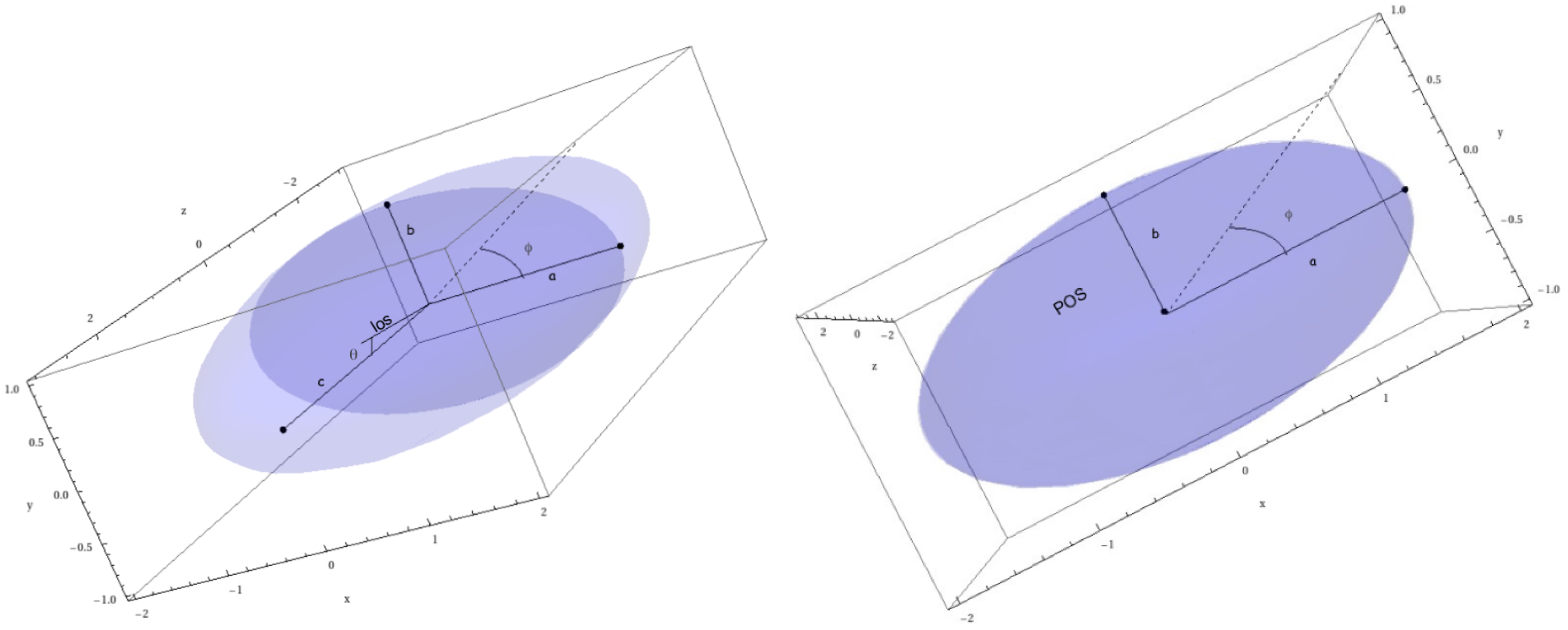
Appendix A.1. β-Model and Triaxial Ellipsoids

In the distribution described by an ellipsoidal triaxial β -model, the electron density of the intracluster gas is assumed to be constant on a family of similar, concentric, coaxial ellipsoids. In a coordinate system relative to GC, the electron density distribution is
n e = n e 0 1 + i = 1 3 v i 2 x i , i n t 2 r c 2 3 β / 2 ,
where x i , i n t is the intrinsic orthogonal coordinate system centred on GC’s barycenter, r c is characteristic length scale distribution at core radius, v i is the inverse of the corresponding core core radius, and n e 0 is the central electron density. If we take the axial ratios e 1 v 1 / v 2 , e 2 v 2 / v 3 , r c 3 = r c / v 3 and taking into account that
x a + y b + z c = r e l l p
such that x 1 = x , x 2 = y , x 3 = z and v 1 = a 1 , v 2 = b 1 , v 3 = c 1 (see Figure A1), we can obtain
n e = n e 0 1 + e 1 2 x 1 , i n t 2 + e 2 2 x 2 , i n t 2 + x 3 , i n t 2 r c 2 3 β / 2
with
β = ν m p σ v 2 k B T e .
Then, the electron density distribution is described by five parameters in a ellipsoidal triaxial β -model: n e 0 , β , e 1 , e 2 and r c 3 .
The projection along the los of the electron density distribution, to a generic power m in the observer coordinate system is given by
l o s n e m ( l ) d l = n e 0 m π Γ ( 3 m β 1 / 2 ) Γ ( 3 m β 2 ) d A θ 3 h 1 + θ 1 2 + e p r o j 2 θ 2 2 θ c , p r o j 2 1 / 2 3 β / 2 ,
where d A is the angular diameter distance in an FRW universe, θ i x i , o b s / d A e p r o j is the projected angular position on the plane of the sky (pos) of the intrinsic orthogonal coordinate system x i , o b s and h is a function of the GC shape and orientation:
h = e 1 2 s i n 2 θ E u s i n 2 φ E u + e 2 2 s i n 2 θ E u c o s 2 φ E u + c o s 2 θ E u ,
such that θ E u and φ E u are the Euler angles in the GC coordinate system (see Figure A1) and
θ c , p r o j θ c 3 e p r o j e 1 e 2 1 / 2 h 1 / 4 .
If we assume that the intracluster medium is described by an isothermal triaxial β -model distribution with m = 1, we obtain
Δ T S Z = Δ T S Z 0 1 + θ 1 2 + e p r o j 2 θ 2 2 θ c , p r o j 2 1 / 2 3 β / 2 ,
where Δ T S Z 0 is the central temperature decrement of SZ effect, which is given by
Δ T S Z 0 T c m b f ( ν , T e ) k B T e m e c 2 n e 0 π d A θ c , p r o j h 4 / 3 e 1 e 2 e p r o j g β 2
and
g α Γ ( 3 α 1 / 2 ) Γ ( 3 α ) .
e p r o j is the axial ratio of the major to minor axes of the observed projected isophotes and θ c , p r o j is the projection on the (pos).
On the other hand, the X-ray surface brightness for intracluster medium with m = 2, is given by
S x = S x 0 1 + θ 1 2 + e p r o j 2 θ 2 2 θ c , p r o j 2 1 / 2 3 β / 2 ,
where the central surface brightness S x 0 is
S x 0 Λ e H ( μ e / μ H ) 4 π ( 1 + z ) 4 n e 0 d A θ c , p r o j h 4 / 3 e 1 e 2 e p r o j g β ,
with μ i ρ / ( n i m p ) the molecular weight.
Figure A1. Ellipsoid coefficients a, b and c, with the los making an angle θ with the z-axis (up). View of the pos with the los oriented along the z-axis (down).
Universe 04 00021 g0a1

Appendix A.2. Galaxy Clusters Data

Table A1 shows us the experimental cosmological distance with triaxial symmetry from De Filippis et al. obtained by the method SZ/X-ray [1]. Column 1 shows the cluster identification name, column 2 gives the corresponding redshift, column 3 is gas temperature, column 4 is central temperature decrement, column 5 is the term of dependence with frequency with relativistic corrections and column 6 show us the experimental cosmological distance. Figure A2 shows us the angular diameter distance vs. redshift and the data sample from De Filippis et al.
Table A1. Galaxy Cluster data set from De Filippis et al. for 25 data points (SZ/X-ray). See [1] for complementary observational information.
Cluster z i k B T e (keV) Δ T SZ 0 ( μ K) f ( ν , T e ) D c | exp ell (Mpc)
MS 1137.5 + 66250.784 5.7 0.7 + 1.3 818 113 + 98 2.00 2479 ± 1023
MS 0451.6 − 03050.550 10.4 0.8 + 1.0 1431 105 + 98 1.87 1073 ± 238
Cl 0016 + 16090.546 7.55 0.58 + 0.72 1242 ± 105 1.89 1635 ± 391
RXJ1347.5 − 11450.451 9.3 0.6 + 0.7 3950 ± 350 1.91 1166 ± 262
A 3700.374 6.6 0.5 + 0.7 785 ± 118 1.96 1231 ± 441
MS 1358.4 + 62450.327 7.48 0.42 + 0.50 784 ± 90 1.88 697 ± 183
A 19950.322 8.59 0.67 + 0.86 1023 + 83 1.91 885 ± 207
A 6110.288 6.6 ± 0.6 853 140 + 120 1.76 934 ± 331
A 6970.282 9.8 ± 0.7 1410 180 + 160 1.89 1099 ± 308
A 18350.252 8.21 0.17 + 0.19 2502 175 + 150 1.93 946 ± 131
A 22610.224 8.82 0.32 + 0.37 1697 ± 200 1.87 1118 ± 283
A 7730.216 9.29 0.36 + 0.41 1260 ± 160 1.76 1465 ± 407
A 21630.202 12.2 0.7 + 1.1 1900 ± 140 1.90 806 ± 163
A 5200.202 8.33 40 + 0.46 662 ± 95 1.93 387 ± 141
A 16890.183 9.66 20 + 0.22 1729 120 + 105 1.86 604 ± 84
A 6650.182 9.03 0.31 + 0.35 728 ± 150 1.87 451 ± 189
A 22180.171 7.05 0.21 + 0.22 731 100 + 125 1.95 809 ± 263
A 14130.142 7.54 0.16 + 0.17 856 ± 110 1.88 478 ± 126
A 21420.091 7.0 ± 0.2 437 ± 25 1.87 335 ± 70
A 4780.088 8.0 ± 0.2 375 ± 28 1.91 448 ± 185
A 16510.084 8.4 ± 0.7 247 ± 30 1.75 749 ± 385
A 4010.074 6.4 ± 0.2 338 ± 20 1.78 369 ± 62
A 3990.072 9.1 ± 0.4 164 ± 21 1.81 165 ± 45
A 22560.058 9.7 ± 0.8 243 ± 29 1.96 242 ± 61
A 16560.023 6.6 ± 0.2 302 ± 48 1.96 103 ± 42
Figure A2. Angular diameter distance vs. redshift for different models with the best fit values from joint analysis (CMB + BAO + SNIa + d A + f g a s s + SGL) and a set of 25 data points from De Filippis et al. (Gray) [1].
Universe 04 00021 g0a2

Appendix B

Appendix B.1. SNIa

We use the Union 2.1 compilation, which contains a sample of 580 data points. We can get the luminosity distance through the relation d L ( z ) = ( 1 + z ) 2 d A ( z ) , then to fit cosmological model by minimizing the χ 2 value defined by
χ S N I a 2 = A B 2 C ,
where
A = i = 1 580 [ μ t h ( z i , p i ) μ o b s ( z i ) ] 2 σ μ i 2 ,
B = i = 1 580 μ t h ( z i , p i ) μ o b s ( z i ) σ μ i 2 ,
C = i = 1 580 1 σ μ i 2 ,
where μ ( z ) 5 log 10 [ d L ( z ) / Mpc ] + 25 is the theoretical value of the distance modulus, and we have marginalized over the nuisance parameter μ 0 and μ o b s .

Appendix B.2. CMB

A standard observational test is the angular scale of sound horizon ( r s ) at the time of decoupling ( z c m b ∼1090), which is encoded in the location of the first peak of the CMB power spectrum l 1 T T . We include CMB information of Planck 13 data [42], whose minimization is given by
χ C M B 2 = X P l a n c k 13 T C c m b 1 X P l a n c k 13 ,
such that
X P l a n c k 13 = l A 301.57 R 1.7407 ω b 0.02228 ,
where ω b = Ω b h 2 . Here, l A is the “acoustic scale” defined as
l A = π d A ( z c m b ) ( 1 + z c m b ) r s ( z c m b ) ,
where d A ( z c m b ) is the angular diameter distance and z c m b is the redshift of decoupling given by [73],
z c m b = 1048 [ 1 + 0.00124 ( Ω b h 2 ) 0.738 ] [ 1 + g 1 ( Ω m h 2 ) g 2 ] ,
g 1 = 0.0783 ( Ω b h 2 ) 0.238 1 + 39.5 ( Ω b h 2 ) 0.763 , g 2 = 0.560 1 + 21.1 ( Ω b h 2 ) 1.81 .
The “shift parameter” R is defined as [74]
R = Ω m c d A ( z c m b ) ( 1 + z c m b ) .
C c m b 1 in Equation (A15) is inverse covariance matrix for ( R , l A , ω b ), which to Planck 13 data is:
C c m b P l a n c k 13 1 = σ i σ j C N o r C o v i , j ,
where σ i = 0.18 , 0.0094 , 0.00030 and normalized covariance matrix is:
C N o r C o v i , j = 1.0000 0.5250 0.4235 0.5250 1.0000 0.6925 0.4235 0.6925 1.0000 .
This test contributes with three data points to the statistical analysis.

Appendix B.3. BAO

The large scale correlation function measured from SDSS, includes a peak that was identified with the expanding spherical wave of baryonic perturbations from acoustic oscillations at recombination, whose current comoving scale corresponds to 150 Mpc. The expected BAO scale depends on the scale of the sound horizon at recombination and on transverse and radial scales at the mean redshift of galaxies in the survey. To obtain constraints on the cosmological model, we begin with χ 2 for WiggleZ BAO data [32], which is given by
χ W i g g l e Z 2 = ( A ¯ o b s A ¯ t h ) C W i g g l e Z 1 ( A ¯ o b s A ¯ t h ) T ,
where A ¯ o b s = ( 0.447 , 0.442 , 0.424 ) is data vector at z = ( 0.44 , 0.60 , 0.73 ) and A ¯ t h ( z , p i ) is given by [75]
A ¯ t h = D V ( z ) Ω m H 0 2 c z ,
in which D V ( z ) is the distance scale defined as
D V ( z ) = 1 H 0 ( 1 + z ) 2 d A ( z ) 2 c z E ( z ) 1 / 3 .
Here, d A ( z ) is the angular diameter distance. Additionally, C W i g g l e Z 1 is the inverse covariance matrix for the WiggleZ data set given by
C W i g g l e Z 1 = 1040.3 807.5 336.8 807.5 3720.3 1551.9 336.8 1551.9 2914.9 .
Similarly, for the SDSS DR7 BAO distance measurements, χ 2 can be expressed as [76]
χ S D S S 2 = ( d ¯ o b s d ¯ t h ) C S D S S 1 ( d ¯ o b s d ¯ t h ) T ,
where d ¯ o b s = ( 0.1905 , 0.1097 ) is the data points at z = 0.2 and z = 0.35 . Here, d ¯ t h ( z d , p i ) denotes the distance ratio
d ¯ t h = r s ( z d ) D V ( z ) ,
in which r s ( z ) is the comoving sound horizon given by
r s ( z ) = c z c s ( z ) H ( z ) d z ,
and c s ( z ) is the sound speed
c s ( z ) = 1 3 ( 1 + R b ¯ / ( 1 + z ) ,
with R b ¯ = 31 , 500 Ω b h 2 ( T C M B / 2.7 K ) 4 and T C M B = 2.726 K. The redshift z d r a g at the baryon drag epoch is fitted with the formula proposed in [77],
z d r a g = 1291 ( Ω m h 2 ) 0.251 1 + 0.659 ( Ω m h 2 ) 0.828 [ 1 + b 1 ( Ω b h 2 ) b 2 ] ,
where
b 1 = 0.313 ( Ω m h 2 ) 0.419 [ 1 + 0.607 ( Ω m h 2 ) 0.674 ]
and
b 2 = 0.238 ( Ω m h 2 ) 0.223 .
Here, C S D S S 1 is the inverse covariance matrix for the SDSS data set given by
C S D S S 1 = 30124 17227 17227 86977 .
For the 6dFGS BAO data [78], there is only one data point at z = 0.106 , and χ 2 is easy to compute
χ 6 d F G S 2 = d z 0.336 0.015 2 .
Additionally, we include measures from the Main Galaxy Sample of Data Release 7 of Sloan Digital Sky Survey (SDSS-MGS) [79] r s / D V ( 0.57 ) = 0.0732 ± 0.0012 . Then, the total χ B A O 2 is given by
χ B A O 2 = χ W i g g l e Z 2 + χ S D S S 2 + χ 6 d F G S 2 + χ S D S S M G S 2 .

References

  1. De Filippis, E.; Sereno, M.; Bautz, M.W.; Longo, G. Measuring the Three-dimensional Structure of Galaxy Clusters. I. Application to a Sample of 25 Clusters. Astrophys. J. 2005, 625, 108–120. [Google Scholar] [CrossRef] [Green Version]
  2. Bonamente, M.; Joy, M.K.; LaRoque, S.J.; Carlstrom, J.E.; Reese, E.D.; Dawson, K.S. Determination of the Cosmic Distance Scale from Sunyaev-Zel’dovich Effect and Chandra X-ray Measurements of High-redshift Galaxy Clusters. Astrophys. J. 2006, 647, 25–54. [Google Scholar] [CrossRef]
  3. Biesiada, M.; Piórkowska, A.; Malec, B. Cosmic equation of state from strong gravitational lensing systems. Mon. Not. R. Astron. Soc. 2010, 406, 1055–1059. [Google Scholar] [CrossRef]
  4. Campigotto, M.C.; Diaferio, A.; Hernandez, X.; Fatibene, L. Strong gravitational lensing in f (χ) = χ3/2 gravity. J. Cosmol. Astropart. Phys. 2017, 2017, 057. [Google Scholar] [CrossRef]
  5. Albrecht, A.; Bernstein, G.; Cahn, R.; Freedman, W.L.; Hewitt, J.; Hu, W.; Huth, J.; Kolb, E.W.; Knox, L.; Mather, J.C.; et al. Report of the Dark Energy Task Force. arXiv, 2006; arXiv:astro-ph/0609591. [Google Scholar]
  6. Frieman, J.A.; Turner, M.S.; Huterer, D. Dark Energy and the Accelerating Universe. Annu. Rev. Astron. Astrophys. 2008, 46, 385–432. [Google Scholar] [CrossRef]
  7. Copeland, E.J.; Sami, M.; Tsujikawa, S. Dynamics of dark energy. Int. J. Mod. Phys. D 2006, 15, 1753–1935. [Google Scholar] [CrossRef]
  8. Weinberg, S. The cosmological constant problem. Rev. Mod. Phys. 1989, 61, 1–22. [Google Scholar] [CrossRef]
  9. Bartelmann, M.; Steinmetz, M.; Weiss, A. Arc statistics with realistic cluster potentials. 2: Influence of cluster asymmetry and substructure. Astron. Astrophys. 1995, 297, 1–12. [Google Scholar]
  10. Sunyaev, R.A.; Zel’dovich, Y.B. The Spectrum of Primordial Radiation, its Distortions and their Significance. Comment Astrophys. Space Phys. 1970, 2, 66–74. [Google Scholar]
  11. Sunyaev, R.A.; Zel’dovich, Y.B. Microwave background radiation as a probe of the contemporary structure and history of the universe. Annu. Rev. Astron. Astrophys. 1980, 18, 537–560. [Google Scholar] [CrossRef]
  12. Itoh, N.; Kohyama, Y.; Nozawa, S. Relativistic Corrections to the Sunyaev–Zeldovich Effect for Clusters of Galaxies. Astrophys. J. 1998, 502, 7–15. [Google Scholar] [CrossRef]
  13. Nozawa, S.; Itoh, N.; Suda, Y.; Ohhata, Y. An improved formula for the relativistic corrections to the kinematical Sunyaev-Zeldovich effect for clusters of galaxies. Nuovo Cimento B 2006, 121, 487–500. [Google Scholar]
  14. Vikhlinin, A.; Kravtsov, A.V.; Burenin, R.A.; Ebeling, H.; Forman, W.R.; Hornstrup, A.; Jones, C.; Murray, S.S.; Nagai, D.; Quintana, H.; et al. Chandra Cluster Cosmology Project III: Cosmological Parameter Constraints. Astrophys. J. 2009, 692, 1060–1074. [Google Scholar] [CrossRef]
  15. Sasaki, S. A New method to estimate cosmological parameters using baryon fraction of clusters of galaxies. Publ. Astron. Soc. Jpn. 1996, 48, L119–L122. [Google Scholar] [CrossRef]
  16. Allen, S.W.; Schmidt, R.W.; Ebeling, H.; Fabian, A.C.; van Speybroeck, L. Constraints on dark energy from Chandra observations of the largest relaxed galaxy clusters. Mon. Not. R. Astron. Soc. 2004, 353, 457–467. [Google Scholar] [CrossRef]
  17. Nesseris, S.; Perivolaropoulos, L. Crossing the Phantom Divide: Theoretical Implications and Observational Status. J. Cosmol. Astropart. Phys. 2007, 2007, 189–198. [Google Scholar] [CrossRef]
  18. Allen, S.W.; Rapetti, D.A.; Schmidt, R.W.; Ebeling, H.; Morris, G.; Fabian, A.C. Improved constraints on dark energy from Chandra X-ray observations of the largest relaxed galaxy clusters. Mon. Not. R. Astron. Soc. 2008, 383, 879–896. [Google Scholar] [CrossRef]
  19. Limousin, M.; Morandi, A.; Sereno, M.; Meneghetti, M.; Ettori, S.; Bartelmann, M.; Verdugo, T. The Three- Dimensional Shapes of Galaxy Clusters. Space Sci. Rev. 2013, 177, 155–194. [Google Scholar] [CrossRef]
  20. Cao, S.; Pan, Y.; Biesiada, M.; Godlowski, W.; Zhu, Z.-H. Constraints on cosmological models from strong gravitational lensing systems. J. Cosmol. Astropart. Phys. 2012, 2012, 140–143. [Google Scholar] [CrossRef]
  21. White, R.E., III; Davis, D.S. X-ray Properties of a Complete Sample of Elliptical Galaxies. Bull. Am. Astron. Soc. 1996, 28, 1323. [Google Scholar]
  22. Narayan, R.; Bartelmann, M. Lectures on Gravitational Lensing. arXiv, 1996; arXiv:astro-ph/9606001. [Google Scholar]
  23. Sereno, M.; Longo, G. Determining cosmological parameters from X-ray measurements of strong lensing clusters. Mon. Non. R. Astron. Soc. 2004, 354, 1255–1262. [Google Scholar] [CrossRef] [Green Version]
  24. Cavaliere, A.; Fusco-Femiano, R. X-rays from hot plasma in clusters of galaxies. Astron. Astrophys. 1976, 49, 137–144. [Google Scholar]
  25. Rosati, P.; Borgani, S.; Norman, C. The Evolution of X-ray Clusters of Galaxies. Annu. Rev. Astron. Astrophys. 2002, 40, 539–577. [Google Scholar] [CrossRef]
  26. Schneider, P.; Ehlers, J.; Falco, E.E. Gravitational Lenses; XIV 560; Springer: Berlin/Heidelberg, Germany; New York, NY, USA, 1992; p. 112. [Google Scholar]
  27. Ono, T.; Masai, K.; Sasaki, S. Cluster Mass Estimate Using Strong Gravitational Lenses Revisited. Publ. Astron. Soc. Jpn. 1999, 51, 91–94. [Google Scholar] [CrossRef]
  28. Yu, H.; Zhu, Z.-H. Combining optical and X-ray observations of galaxy clusters to constrain cosmological parameters. Res. Astron. Astrophys. 2011, 11, 776–786. [Google Scholar] [CrossRef]
  29. Suzuki, N.; Rubin, D.; Lidman, C.; Aldering, G.; Amanullah, R.; Barbary, K.; Barrientos, L.F.; Botyanszki, J.; Brodwin, M.; Connolly, N.; et al. The Hubble Space Telescope Cluster Supernova Survey: V. Improving the Dark Energy Constraints Above z>1 and Building an Early-Type-Hosted Supernova Sample. Astrophys. J. 2012, 746, 85. [Google Scholar] [CrossRef]
  30. Wang, Y.; Wang, S. Distance priors from Planck and dark energy constraints from current data. Phys. Rev. D 2013, 88, 043522. [Google Scholar] [CrossRef]
  31. Anderson, L.; Aubourg, E.; Bailey, S.; Bizyaev, D.; Blanton, M.; Bolton, A.S.; Brinkmann, J.; Burden, A.; Cuesta, A.J.; Brownstein, J.R.; et al. The clustering of galaxies in the SDSS-III Baryon Oscillation Spectroscopic Survey: Baryon Acoustic Oscillations in the Data Release 9 Spectroscopic Galaxy Sample. Mon. Non. R. Astron. Soc. 2012, 427, 3435–3467. [Google Scholar] [CrossRef] [Green Version]
  32. Blake, C.; Kazin, E.A.; Beutler, F.; Davis, T.M.; Parkinson, D.; Brough, S.; Colless, M.; Contreras, C.; Couch, W.; Croom, S.; et al. The WiggleZ Dark Energy Survey: mapping the distance-redshift relation with baryon acoustic oscillations. Mon. Non. R. Astron. Soc. 2011, 418, 1707–1724. [Google Scholar] [CrossRef]
  33. Shi, K.; Huang, Y.; Lu, T. A comprehensive comparison of cosmological models from latest observational data. Mon. Non. R. Astron. Soc. 2012, 426, 2452–2462. [Google Scholar] [CrossRef]
  34. Andrae, R.; Schulze-Hartung, T.; Melchior, P. Dos and don’ts of reduced chi-squared. arXiv, 2010; arXiv:1012.3754. [Google Scholar]
  35. Albrecht, A.; Amendola, L.; Bernstein, G.; Clowe, D.; Eisenstein, D.; Guzzo, L.; Hirata, C.; Huterer, D.; Kirshner, R.; Kolb, E.; et al. Findings of the Joint Dark Energy Mission Figure of Merit Science Working Group. arXiv, 2009; arXiv:0901.0721. [Google Scholar]
  36. Wolz, L.; Kilbinger, M.; Weller, J.; Giannantonio, T. On the validity of cosmological Fisher matrix forecasts. J. Cosmol. Astropart. Phys. 2012, 2012, 009. [Google Scholar] [CrossRef]
  37. Akaike, H. A New Look at the Statistical Model Identification. IEEE Trans. Autom. Control 1974, 19, 716–723. [Google Scholar] [CrossRef]
  38. Schwarz, G. Estimating the Dimension of a Model. Ann. Stat. 1978, 6, 471–474. [Google Scholar] [CrossRef]
  39. Liddle, A.R. How many cosmological parameters? Mon. Non. R. Astron. Soc. 2004, 351, L49–L53. [Google Scholar] [CrossRef]
  40. Burnham, K.P.; Anderson, D.R. Model Selection and Multimodel Inference. Technometrics 2003, 45, 181. [Google Scholar]
  41. Hogg, D.W. Distance measures in cosmology. arXiv, 1999; arXiv:astro-ph/9905116. [Google Scholar]
  42. Planck Collaboration; Ade, P.A.R.; Aghanim, N.; Arnaud, M.; Arroja, F.; Ashdown, M.; Aumont, J.; Baccigalupi, C.; Ballardini, M.; Banday, A.J.; et al. Planck 2013 results. XVI. Cosmological parameters. Astron. Astrophys. 2014, 571, A16. [Google Scholar]
  43. Chevallier, M.; Polarski, D. Accelerating Universes with Scaling Dark Matter. Int. J. Mod. Phys. D 2001, 10, 213–223. [Google Scholar] [CrossRef]
  44. Linder, E.V. Mapping the Dark Energy Equation of State. Phys. Rev. Lett. 2003, 90, 091301. [Google Scholar] [CrossRef] [PubMed]
  45. Wang, B.; Abdalla, E.; Atrio-Barandela, F.; Pavón, D. Dark Matter and Dark Energy Interactions: Theoretical Challenges, Cosmological Implications and Observational Signatures. Rep. Prog. Phys. 2016, 79, 096901. [Google Scholar] [CrossRef] [PubMed]
  46. Bolotin, Y.L.; Kostenko, A.; Lemets, O.A.; Yerokhin, D.A. Cosmological Evolution With Interaction Between Dark Energy And Dark Matter. Int. J. Mod. Phys. D 2015, 24, 1530007. [Google Scholar] [CrossRef]
  47. Kumar, S.; Nunes, R.C. Probing the interaction between dark matter and dark energy in the presence of massive neutrinos. Phys. Rev. D 2016, 94, 123511. [Google Scholar] [CrossRef]
  48. Kumar, S.; Nunes, R.C. Echo of interactions in the dark sector. Phys. Rev. D 2017, 96, 103511. [Google Scholar] [CrossRef]
  49. Nunes, R.C.; Pan, S.; Saridakis, E.N. New constraints on interacting dark energy from cosmic chronometers. Phys. Rev. D 2016, 94, 023508. [Google Scholar] [CrossRef]
  50. Richarte, M.G.; Xu, L. Exploring a new interaction between dark matter and dark energy using the growth rate of structure. arXiv, 2015; arXiv:1506.02518. [Google Scholar]
  51. Sharov, G.S.; Bhattacharya, S.; Pan, S.; Nunes, R.C.; Chakraborty, S. A new interacting two fluid model and its consequences. Mon. Non. R. Astron. Soc. 2017, 466, 3497–3506. [Google Scholar] [CrossRef]
  52. Salvatelli, V.; Said, N.; Bruni, M.; Melchiorri, A.; Wands, D. Indications of a late-time interaction in the dark sector. Phys. Rev. Lett. 2014, 113, 181301. [Google Scholar] [CrossRef] [PubMed]
  53. Wang, P.; Meng, X.-H. Can vacuum decay in our universe? Class. Quantum Gravity 2005, 22, 283–294. [Google Scholar] [CrossRef]
  54. Costa, F.E.M.; Barboza, E.M., Jr.; Alcaniz, J.S. Cosmology with interaction in the dark sector. Phys. Rev. D 2009, 79, 127302. [Google Scholar] [CrossRef]
  55. Nunes, R.C.; Barboza, E.M. Dark matter-dark energy interaction for a time-dependent equation of state. Gen. Relativ. Gravit. 2014, 46, 1820. [Google Scholar] [CrossRef]
  56. Yang, W.; Banerjee, N.; Pan, S. Constraining a dark matter and dark energy interaction scenario with a dynamical equation of state. arXiv, 2017; arXiv:1705.09278. [Google Scholar]
  57. Steinhardt, P.J.; Wang, L.; Zlatev, I. Cosmological tracking solutions. Phys. Rev. D 1999, 59, 123504. [Google Scholar] [CrossRef]
  58. Doran, M.; Robbers, G. Early Dark Energy Cosmologies. J. Cosmol. Astropart. Phys. 2006, 6, 573–583. [Google Scholar] [CrossRef]
  59. Sandage, A. The Change of redshift and Apparent Luminosity of Galaxies due to the Deceleration of Selected Expanding Universes. Astrophys. J. 1962, 136, 319–333. [Google Scholar] [CrossRef]
  60. Bolotin, Y.L.; Erokhin, D.A.; Lemets, O.A. Expanding Universe: Slowdown or speedup? Phys. Uspekhi 2012, 55, 941–986. [Google Scholar] [CrossRef]
  61. Perlmutter, S.; Aldering, G.; Goldhaber, G.; Knop, R.A.; Nugent, P.; Castro, P.G.; Deustua, S.; Fabbro, S.; Goobar, A.; Groom, D.E.; et al. Measurements of Omega and Lambda from 42 High-Redshift Supernovae. Astrophys. J. 1999, 517, 565–586. [Google Scholar] [CrossRef]
  62. Riess, A.G.; Filippenko, A.V.; Challis, P.; Clocchiatti, A.; Diercks, A. Observational Evidence from Supernovae for an Accelerating Universe and a Cosmological Constant. Astron. J. 1998, 116, 1009–1038. [Google Scholar] [CrossRef]
  63. Barrow, J.D.; Bean, R.; Magueijo, J. Can the Universe escape eternal acceleration? Mon. Non. R. Astron. Soc. 2000, 316, L41–L44. [Google Scholar] [CrossRef]
  64. Guimarães, A.C.C.; Lima, J.A.S. Could the cosmic acceleration be transient? A cosmographic evaluation. Class. Quantum Gravity 2011, 28, 125026. [Google Scholar] [CrossRef]
  65. Li, Z.; Wu, P.; Yu, H. Examining the cosmic acceleration with the latest Union2 supernova data. Phys. Lett. B 2011, 695, 1–8. [Google Scholar] [CrossRef]
  66. Shafieloo, A.; Sahni, V.; Starobinsky, A.A. Is cosmic acceleration slowing down? Phys. Rev. D 2009, 80, 101301. [Google Scholar] [CrossRef]
  67. Cárdenas, V.H.; Bernal, C.; Bonilla, A. Cosmic slowing down of acceleration using fgas. Mon. Non. R. Astron. Soc. 2013, 433, 3534–3538. [Google Scholar] [CrossRef]
  68. Magaña, J.; Motta, V.; Cárdenas, V.H.; Foëx, G. Testing cosmic acceleration for w(z) parameterizations using fgas measurements in galaxy clusters. Mon. Non. R. Astron. Soc. 2017, 469, 47–61. [Google Scholar] [CrossRef]
  69. Bonilla Rivera, A.; García Farieta, J. Exploring the Dark Universe: Constraint on dynamical dark energy models from CMB, BAO and Growth Rate Measurements. arXiv, 2016; arXiv:1605.01984. [Google Scholar]
  70. Pan, S.; Chakraborty, S. Will there be future deceleration? A study of particle creation mechanism in non-equilibrium thermodynamics. Adv. High Energy Phys. 2015, 2015, 654025. [Google Scholar] [CrossRef]
  71. Chen, X.-M.; Gong, Y.; Saridakis, E.N. The Transient Acceleration from Time-Dependent Interacting Dark Energy Models. Int. J. Theor. Phys. 2014, 53, 469–481. [Google Scholar] [CrossRef]
  72. Carvalho, F.C.; Alcaniz, J.S.; Lima, J.A.S.; Silva, R. Scalar-field-dominated cosmology with a transient accelerating phase. Phys. Rev. Lett. 2006, 97, 081301. [Google Scholar] [CrossRef] [PubMed]
  73. Hu, W.; Sugiyama, N. Small Scale Cosmological Perturbations: An Analytic Approach. Astrophys. J. 1996, 471, 542–570. [Google Scholar] [CrossRef]
  74. Bond, J.R.; Efstathiou, G.; Tegmark, M. Forecasting Cosmic Parameter Errors from Microwave Background Anisotropy Experiments. Mon. Non. R. Astron. Soc. 1997, 291, L33–L41. [Google Scholar]
  75. Eisenstein, D.J.; Zehavi, I.; Hogg, D.W.; Scoccimarro, R.; Blanton, M.R.; Nichol, R.C.; Scranton, R.; Seo, H.; Tegmark, M.; Zheng, Z.; et al. Detection of the Baryon Acoustic Peak in the Large-Scale Correlation Function of SDSS Luminous Red Galaxies. Astrophys. J. 2005, 633, 560–574. [Google Scholar] [CrossRef]
  76. Percival, W.J.; Reid, B.A.; Eisenstein, D.J.; Bahcall, N.A.; Budavari, T.; Frieman, J.A.; Fukugita, M.; Gunn, J.E.; Lupton, R.H.; Mckay, T.A.; et al. Baryon Acoustic Oscillations in the Sloan Digital Sky Survey Data Release 7 Galaxy Sample. Mon. Non. R. Astron. Soc. 2010, 401, 2148–2168. [Google Scholar] [CrossRef] [Green Version]
  77. Eisenstein, D.J.; Hu, W. Baryonic Features in the Matter Transfer Function. Astrophys. J. 1998, 496, 605–614. [Google Scholar] [CrossRef]
  78. Beutler, F.; Blake, C.; Colless, M.; Heath Jones, D.; Staveley-Smith, L.; Campbell, L.; Parker, Q.; Saunders, W.; Watson, F. The 6dF Galaxy Survey: baryon acoustic oscillations and the local Hubble constant. Mon. Non. R. Astron. Soc. 2011, 416, 3017–3032. [Google Scholar] [CrossRef]
  79. Anderson, L.; Aubourg, E.; Bailey, S.; Beutler, F.; Bhardwaj, V.; Blanton, M.; Bolton, A.S.; Brinkmann, J.; Brownstein, J.R.; Burden, A.; et al. The clustering of galaxies in the SDSS-III Baryon Oscillation Spectroscopic Survey: Baryon acoustic oscillations in the Data Releases 10 and 11 Galaxy samples. Mon. Non. R. Astron. Soc. 2014, 441, 24–60. [Google Scholar] [CrossRef] [Green Version]
1
Even though GC forms at the same time, they can have different evolution and thus different gas fractions. To preserve the constancy of the baryon fraction with redshift to mimic the relative cosmic abundance, GCs have to be selected among the most massive and relaxed ones at each epoch.
2
The pressure gradient force of an isothermal gas with temperature T X is balanced by the gravity in GC.
3
Specifically, a hydrostatic isothermal spherical symmetric β m o d e l .
4
For an unbiased estimator, If all the parameters are assumed to be known (in other words, if we don’t marginalize over any other parameters), then the minimal expected error is σ i = 1 / F i j .
Figure 1. 1σ and 2σ two-dimensional CL contours of DE cosmological models discussed, where the main results are shown using the combined analysis (CMB + BAO + SNIa + dA + fgass + SGL).
Universe 04 00021 g001aUniverse 04 00021 g001b
Figure 2. Deceleration parameter vs. redshift using only GC data ( d A + f g a s ). The transition redshift z t between phases decelerated-accelerated ( q ( z t ) = 0 ) and the current value of deceleration parameter q 0 are shown for Λ C D M ( z t 0.86 , q 0 = 0.76 ), ω C D M ( z t 0.86 , q 0 = 0.76 ), CPL ( z t 1.32 , q 0 = 0.35 ), IDE ( z t 9.78 , q 0 = 0.50 ) and EDE ( z t 1.22 , q 0 = 0.17 ). Notice the strange behavior of the deceleration parameter to later times for models of dynamical DE models CPL, IDE and EDE.
Universe 04 00021 g002
Figure 3. Jerk parameter vs. redshift using only GC data ( d A + f g a s ). For cosmological models CPL, IDE and EDE we can observe a strong deviation from Λ C D M at present, while for w C D M this does not happen.
Universe 04 00021 g003
Table 1. Summary of the best fit values for Λ C D M model.
ParameterCMB + BAO + SNIaCMB + BAO + SNIa + d A + f gass + SGL
h 0.6858 ± 0.0095 0.7063 ± 0.0067
Ω m 0.2981 ± 0.0093 0.2839 ± 0.0046
Ω k 0.0011 ± 0.0031 0.0048 ± 0.0024
Ω b 0.0475 ± 0.0014 0.04411 ± 0.00099
χ m i n 2 565.686777.256
Table 2. Summary of the best fit values for wCDM model.
ParameterCMB + BAO + SNIaCMB + BAO + SNIa + d A + f gass + SGL
h 0.6897 ± 0.0098 0.7080 ± 0.0070
Ω m 0.2964 ± 0.0093 0.2839 ± 0.0049
Ω k 0.0028 ± 0.0033 0.0007 ± 0.0028
ω 1.057 ± 0.041 1.086 ± 0.038
Ω b 0.0468 ± 0.0014 0.0437 ± 0.0010
χ m i n 2 563.953772.283
Table 3. Summary of the best fit values for the CPL model.
ParameterCMB + BAO + SNIaCMB + BAO + SNIa + d A + f gass + SGL
h 0.688 ± 0.011 0.7073 ± 0.0075
Ω m 0.297 ± 0.010 0.2856 ± 0.0059
Ω k 0.0054 ± 0.0055 0.0017 ± 0.0040
w 0 0.97 ± 0.19 0.97 ± 0.15
w 1 0.50 ± 1.13 0.71 ± 0.95
Ω b 0.0470 ± 0.0015 0.0439 ± 0.0011
χ m i n 2 563.854771.481
Table 4. Summary of the best fit values for the IDE model.
ParameterCMB + BAO + SNIaCMB + BAO + SNIa + d A + f gass + SGL
h 0.703 ± 0.015 0.7165 ± 0.0092
Ω m 0.2963 ± 0.0092 0.2844 ± 0.0049
Ω k 0.0048 ± 0.0036 0.0022 ± 0.0029
w x 1.059 ± 0.042 1.074 ± 0.038
δ 0.0048 ± 0.0049 0.0041 ± 0.0036
Ω b 0.0451 ± 0.0019 0.0428 ± 0.0011
χ m i n 2 563.960771.442
Table 5. Summary of the best fit values for the EDE model.
ParameterCMB + BAO + SNIaCMB + BAO + SNIa + d A + f gass + SGL
h 0.723 ± 0.019 0.7154 ± 0.0099
Ω m 0.295 ± 0.010 0.2839 ± 0.0050
Ω k 0.0072 ± 0.0068 0.0032 ± 0.0035
Ω e 0.043 ± 0.029 0.012 ± 0.016
w 0 1.113 ± 0.061 1.087 ± 0.040
Ω b 0.0425 ± 0.0023 0.0429 ± 0.0012
χ m i n 2 564.275771.697
Table 6. AIC and BIC for different DE models using the combined analysis (CMB + BAO + SNIa + d A + f g a s s + SGL), where N = 737 and χ r e d 2 = χ m i n 2 / ν .
Modeld χ red 2 AIC Δ AIC BIC Δ BIC
Λ C D M 41.060785.2562.973803.6660.000
ω C D M 51.055782.2830.000805.2951.626
CPL61.055783.4811.198811.0967.430
IDE61.055783.4421.159811.0577.391
EDE61.055783.6971.414811.3127.646
Table 7. The best fit values for the free parameters using data from GC ( d A + f g a s ).
Model χ red 2 Parameters
Λ C D M 1.11 h = 0.722 ± 0.012 , Ω m = 0.2640 ± 0.0093 , Ω k = 0.13 ± 0.16 , Ω b = 0.0410 ± 0.0014
ω C D M 1.11 h = 0.722 ± 0.012 , Ω m = 0.2685 ± 0.0093 , Ω k = 0.14 ± 0.88 , w = 0.99 ± 0.73 , Ω b = 0.0409 ± 0.0015 .
CPL1.14 h = 0.721 ± 0.011 , Ω m = 0.274 ± 0.013 , Ω k = 0.5 ± 1.8 , w 0 = 0.60 ± 0.50 , w 1 = 1.5 ± 2.2 , Ω b = 0.0411 ± 0.0014 .
IDE1.14 h = 0.721 ± 0.011 , Ω m = 0.274 ± 0.012 , Ω k = 0.2 ± 2.5 , w x = 1.1 ± 3.1 , δ = 3.9 ± 13.0 , Ω b = 0.0411 ± 0.0015 .
EDE1.14 h = 0.720 ± 0.012 , Ω m = 0.276 ± 0.014 , Ω k = 0.3 ± 1.7 , w 0 = 0.8 ± 1.7 , Ω e = 1.1 ± 1.7 , Ω b = 0.0412 ± 0.0015 .

