Weak Lensing Data and Condensed Neutrino Objects

1
Booz-Allen-Hamilton Inc., McLean, VA 22102, USA
2
Independent Researcher, Springfield, VA 22150, USA
*
Author to whom correspondence should be addressed.
Universe 2017, 3(4), 81; https://doi.org/10.3390/universe3040081
Submission received: 24 October 2017
/
Revised: 13 November 2017
/
Accepted: 15 November 2017
/
Published: 23 November 2017
(This article belongs to the Special Issue Progress in Cosmology in the Centenary of the 1917 Einstein Paper)
Abstract
:Condensed Neutrino Objects (CNO) are a candidate for the Dark Matter which everyone has been looking for. In this article, from Albert Einstein’s original 1911 and 1917 papers, we begin the journey from weak lensing data to neutrino signatures. New research results include an Einasto density profile that fits to a range of candidate degenerate neutrino masses, goodness-of-fit test results for our functional CNO mass/radius relationship which fits to available weak lensing data, and new results based on revised constraints for the CNO that our Local Group of galaxies is embedded in.
1. Introduction
In 1911, A. Einstein [1] used classical theory to derive the gravitational bending of light. This 1911 answer was wrong by a factor of 2. In 1916, he published his compendium General Theory of Relativity [2] which, in the weak field approximation, finally led to the correct light bending formula. Modern cosmology was born in 1917 [3] with the publication of Einstein’s static cosmology. We now have experimental evidence that space–time is flat [4].
Einstein’s gravitational lensing and flat space–time together set the stage for potentially one of the most important discoveries in science: the identification of the enigmatic Dark Matter. This non-luminous substance is thought to be about 24% of the mass density of the universe, based on cosmic microwave background fluctuations measured by the Wilkerson Microwave Anisotropy Probe [4]. The gravitational bending of light with flat space–time will allow us to identify Dark Matter-critical signatures, discussed below in this paper.
Modern Dark Matter was first hypothesized to exist by F. Zwicky [5] who used the Virial Theorem applied to the Comma Cluster of Galaxies to show that individual galaxies’ velocity dispersion was too large to be explained from the gravity of the observable luminous matter present. Later in this paper, we will remark that a single galaxy embedded within a Condensed Neutrino Object (CNO) actually undergoes simple harmonic oscillation. Depending on their distance from the CNO center, their individual speeds can indeed be very high. Because Dark Matter has no observed electric charge or opacity (meaning it is transparent to light), the only manifestation of its existence is its gravitational effects, in particular the gravitational bending of light. Extensive reviews of Dark Matter weak lensing techniques are available in the literature (e.g., Kitching [6]). Actual Dark Matter particle searches at the “Conseil Européen pour la Recherche Nucléaire” Large Hadron Collider (CERN LHC) were reviewed by Kahlhoefer [7]. The Standard Cosmological Model which predicts the relative percentage of Dark Matter in the universe was recently critically reviewed in [8]. Reviews of Dark Matter can be found in [9] and [10]. The latter reference reviews the main theoretical and experimental achievements for Dark Matter vis-a-vis cosmology and astrophysics, while the former reference is intended for non-specialists.
The key physics associated with Dark Matter is its equation of state (EOS). An object made up of any type of matter has an EOS, including Black Holes. The EOS derives the relationship of an object’s mass to its radius. We will show below that CNO (if they exist) are the largest and most massive objects in the universe, being thousands of times more massive than the Milky Way galaxy and so large that CNO can easily embed a whole cluster of galaxies.
If Dark Matter is made up of boson particles, they must have an internal energy source. Since these bosons would have been created at the time of the Big Bang, the expansion of the Universe would have cooled them down to very low energies. They would then fall into the lowest energy state and their aggregate cloud would be hydro-statically unstable; they would end up as a Black Hole. For these reasons, bosons are not good candidates for the particle constituent of Dark Matter.
Fermions satisfy the Pauli Exclusion Principle (PEP) because they are in the totally asymmetric representation of the identical particle permutation group. That means that when Fermions condense, they become ordered into increasing momentum states and thus exert an internal pressure. The PEP is the reason your hand cannot penetrate a table’s surface. Therefore, Fermions are a natural candidate for the particle of Dark Matter. But which Fermions?
Cosmological neutrinos and anti-neutrinos were created in the original Big Bang, in almost unlimited numbers1. If they should condense, they would make excellent Dark Matter particle candidates. However, certain details come into play. What would be the mechanism for neutrinos and anti-neutrinos to lose their energy and actually condense? The expansion of space–time has caused cosmological photons to become very cold, but they have not condensed. Clearly the expansion of the universe is not sufficient by itself for neutrino and anti-neutrino condensation.
2. Neutrino Magnetic Moment Power Loss
If neutrinos were their own anti-neutrinos (Majorana neutrinos) then they could not have a permanent magnetic dipole moment, because this quantum number changes sign under the operation of charge conjugation. Dirac neutrinos do not have this issue, and we expect that Dirac neutrinos and their distinct anti-neutrinos will have a finite-sized magnetic dipole moment. In reference [12], the relativistic power loss for magnetic dipole radiation was computed to be
where β = v/c,2 μ = dipole moment, with the dot (˙) above the vector arrow (→) as is usual to indicate the time derivative (), while the double dot is the double time derivative (). The first term is the leading order term in the power loss physics formula and it does not depend on the value of the neutrino (anti-neutrino) dipole moment. Instead, it depends on the square of the time derivative, which has values from zero to infinity. Parenthetically, the power of γ in this leading term is even higher than the γ power in the famous Liénard formula for charged particle power loss [13]. Elementary particles cannot change their dipole moment scalar value, but in fluctuating magnetic fields, their moments will change their direction. When they flip spin direction and align with an external magnetic field, they emit a photon3. It is this radiation that Equation (1) is describing. There is no limit to dipole radiation loss save a limit on the time dependence of the external magnetic field. In the hot Early Universe, chaotic, massive and turbulent magnetic fields are expected to have existed [14]. The radiation loss would lead to neutrinos that were out of equilibrium with baryonic matter (the ramifications are described below). The cooling (expansion) of the Universe along with dipole radiation power loss could result in cosmological neutrinos and anti-neutrinos condensing.
3. Condensed Neutrinos is an Idea Many Decades Old
The history of this idea is given in reference [15]. What are lacking in previous papers are a condensation mechanism, theoretical signatures, and observational data supporting the idea. In particular, humans may be moving in Dark Matter because it seems to be present in the Milky Way [16], but how can this be proven? All this is missing in the previous papers. In their defense, it is impossible to obtain the theoretical signatures without the modern knowledge of the neutrino mass matrix. It turns out that a key terrestrial physics experiment, KArlsruhe TRItium Neutrino (KATRIN) [17], can now make a potentially seminal contribution, because of the aforementioned signature data. This is explained in detail below.
As stated, one critical constraint for Equation (1) to be valid, is that the neutrinos must be of the Dirac-type, not Majorana-type. If neutrinos were Majorana, then neutrinoless double beta decay, n + n −> p + p + e + e (Figure 1) would occur.
No experiment has ever seen this type of radioactivity. Based on current experimental evidence, the lifetime for this decay has a lower limit many orders of magnitude longer than the age of the Universe [18]. The assumption that neutrinos and their anti-neutrinos are of the Dirac-type is consistent with all available experimental data.
Another critical constraint for Equation (1) is that neutrinos must have mass. The existence of neutrino flavor mixing means that neutrinos have mass, and this experimental discovery was rewarded with the 2015 Nobel Prize in Physics [19]. The Particle Data Handbook gives an upper bound to the electron anti-neutrino of <2 eV/c2 [11].5 Mass mixing is only possible if the neutrinos have very close spacing of their masses:
where . We will show below that all these different and diverse pieces of information will come into play like the individual instruments coming together in a master symphony.
4. Neutrino Equation of State
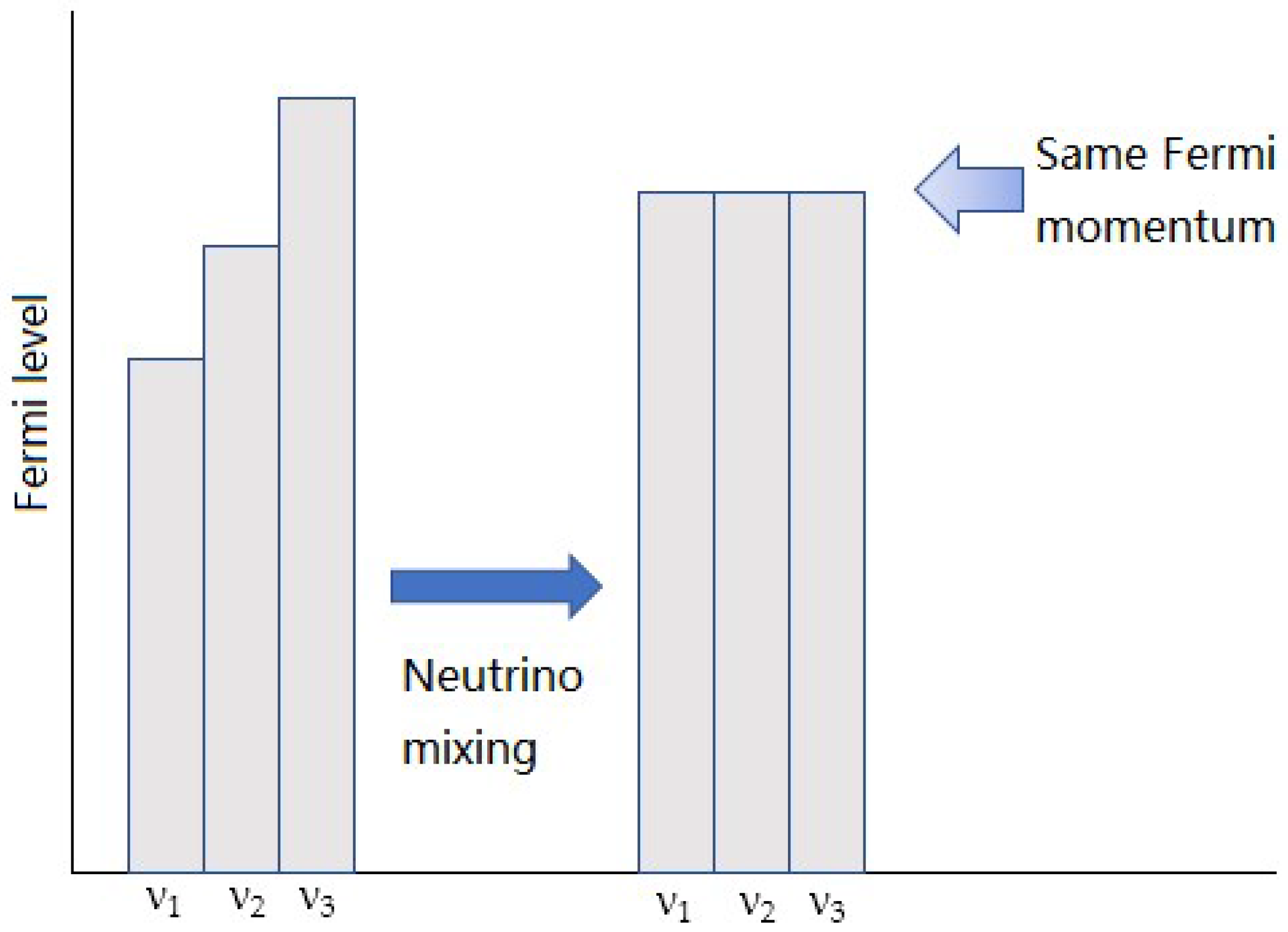
Should the cosmological neutrinos be Dirac-type, then condensation at the present time will result in essentially near-zero temperature Fermi matter, which we describe by their condensation Fermi momentum. Designating the three neutrino flavors by ν1, ν2, ν3, the three neutrino flavors may initially have three different Fermi momenta, Figure 2. However, mixing causes the higher Fermi levels to vacate and fill unfilled other flavor neutrino levels, resulting in the same Fermi momentum for all three neutrino flavors. The same is true for the three flavor anti-neutrinos. Thus, the most general Condensed Neutrino Object will be described by two Fermi momenta. However, spectroscopically, no measurement can be made to differentiate these different types and, since we are only interested in the mass and radius of these large objects, we describe them by setting the neutrino Fermi momentum equal to the anti-neutrino Fermi momentum. Furthermore, since the neutrino masses are nearly identical, we use one neutrino mass mν for all six flavors and call it the “neutrino degenerate mass”. Thus, the equation of state will be a Fermion fluid with common mass mν and 6 flavors (3 neutrino and 3 anti-neutrino), each having 2 degrees of freedom from their spin vector direction, and each flavor contributing to the pressure. The CNO EOS [12] is
where x = pf/mνc; pf = Fermi momentum; and with c = speed of light (as before). The equation of hydro-statistic equilibrium is
The boundary conditions are: x = x(0) at r = 0 and dx/dr = 0 at r = 0. Only the first boundary condition differentiates the different CNO once the degenerate mν is determined. Observationally: x(0) << 1. The value of mν has to be determined by observational astronomical data, and be consistent with any future direct measurement of any neutrino or anti-neutrino flavor.
5. CNO are Stable Objects
The CNO are forbidden to decay into electron-positron pairs by energy conservation, since the neutrinos are non-relativistic (x(0) << 1). Their decay into photon pairs is an extremely small cross section. As already stated, they have no opacity (one can see right through them) and the only clue to their existence is their gravitational potential. Solutions to Equation (4) give spherical CNO, but there may be situations where the spherical symmetry is perturbed (as discussed below).
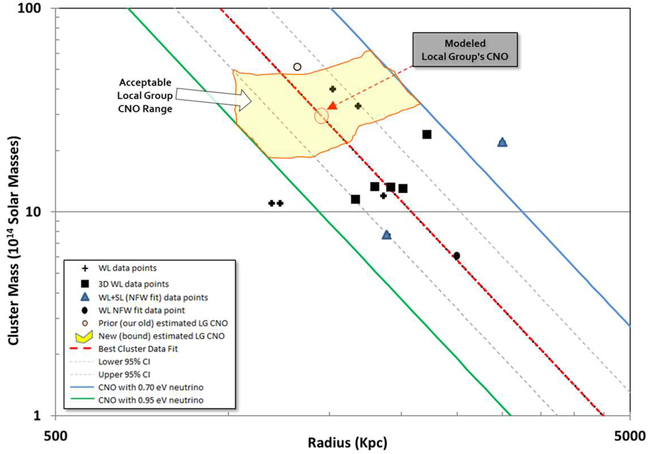
We will show below that the Local Group of Galaxies (M31, M33 and the Milky Way) is embedded in one of these objects (we will call it CNO_LG). This will be demonstrated by determining the origin and radius, a seemingly impossible task. The question is then, “How old are these objects?” One can model galaxy formation and cluster-of-galaxies formation in the potential well of a CNO, and determine whether the CNO act as a catalyst (by capturing and compressing baryonic matter in the well) for galaxy building; if so, then the conclusion would be that the CNO are very ancient objects, predating most galaxies. In Table 1, we give solutions to Equation (4), using the following notation: Mtotal is the total mass in solar masses (MΘ), ly (light years), Ω (gravitational potential energy of formation), RS (Schwarzschild radius).
Table 1 shows that CNO are the largest and most massive objects in the universe. It also discloses the key signature: degenerate Fermi matter EOS, whether neutron stars (nucleons) or white dwarfs (electrons), have the distinctive property that the more massive the object is, the smaller the radius it has. This is in counter-distinction to iron–silicate EOS such as earth’s. We used gravitational lensing (gravitational bending of light) and flat space–time to measure the mass and radii of Dark Matter objects embedding galaxy clusters and showed that the curve had a negative slope, as predicted by Table 1 [20]. The negative slope, of course, depends on the value of the degenerate neutrino mass mν. By fitting the Dark Matter observational data, an approximate value of mν can be predicted. It is this predicted value that the KATRIN experiment [17] should use, since its team is directly measuring the mass of the electron anti-neutrino, which should be nearly the value of the common degenerate neutrino mass.
The second boundary condition dx/dr = 0 at r = 0 means that the degenerate Fermion fluid has a finite density at the center. This is reflected in the solution graphs of Figure 3 below. All Fermion degenerate fluids are of finite density. Section 7 describes recent work in modeling CNO density solutions with Einasto density profiles.
The CNO are predicted to have interesting properties which are consistent with Dark Matter observations, some of which are listed in Table 2.
6. Materials and Methods
In previously published results, Mathematica® from Wolfram Research was used to solve numerically the hydrostatic equation for Condensed Neutrino Objects. These equations and details were sufficient for other researchers to replicate, and were originally provided in [12]. The Dark Matter signature for CNO with the methods and arguments used to identify and constrain the applicable data were provided in [20]. A solution for our Local Group CNO, with sufficient detail for replication, were first obtained using the quite familiar Monte Carlo method and was described in [21].
Updates to this prior work, and the new work provided here includes identifying and including additional applicable weak lensing observational data, and using Mathematica® to provide non-linear fits of our theoretical density profiles to the Einasto density profile for a wide range of potential degenerate neutrino mass and x(0) solution pairs. Mathematica® was also used to provide new results for a number of commonly used goodness-of-fit tests for our functional form (shown below—the fit derivation is found in the appendix of [20]). We now propose a comparison of our initial Monte Carlo (FORTRAN) results with our results from a Latin Hypercube implementation in C++, providing a comparison of these results for the center solutions of the CNO embedding the Local Group of galaxies on a starfield night sky. We also include a revised plot of potential/applicable CNO solutions for the CNO_LG with the identified weak lensing data.
7. Updated and New Results
This section is divided into subsections covering each of the updated or new research results, as discussed in the prior section.
7.1. Einasto Density Profile Fits
Originally published in simple linear form as Figure 2 by the authors in [20], Figure 3 below revises that figure to now include fits to the Einasto density model Equation (5). See for example references [22,23] with plots in linear-linear form, as well as the more familiar log-log format.
where α is the shape parameter, and are the density and radius at .
In the log-log version of the Einasto density profile fits, it can be seen that when using a degenerate mass of 0.8 eV/c2 the fit to the data overlap the theoretical values extremely well up to a CNO radius ~1.7 Mpc. Beyond those values, the theoretical density/radius values were generally less than (i.e., fall short of) the corresponding Einasto profile density fit’s value.
Table 3 provides Einasto density fit parameters for three cases of degenerate neutrino masses (0.7, 0.8 and 0.95 eV/c2) to theoretical spherical CNOs for various x(0) boundary conditions. Rmax is the spherical CNO’s outer boundary for a given degenerate neutrino mass and x(0) is the (internal) boundary condition. Also of note in Table 3 is the nearly constant shape parameter with values of ~2.20 across a range of degenerate neutrino masses and x(0) constraint parameters. This is an important finding that directly contradicts Einasto fit values from N-body modeling studies and will be revisited in more detail in the discussion section.
7.2. Dark Matter Galaxy Cluster Data
After routinely scouring the literature for applicable galaxy cluster data with virial mass and radii estimates (see arguments in [20] as to the reason for not using x-ray derived data points) we present additional data in Table 4 using the following nomenclature/notes: (1) WL is weak lensing data that uses an estimated Dark Matter velocity dispersion based on tangential shear measurements. The Coma analysis used weak lensing combined with the Navarro–Frenk–White (NFW) fit to obtain their mass estimates; (2) SL + WL (NFW fit) is strong lensing and weak lensing data that used the NFW density profile to fit a mass profile; and (3) 3D WL indicates the three-dimensional mass within a sphere of a fixed mean interior over-density with respect to the critical density of the universe at the cluster’s redshift z.
This data set is plotted in Figure 4 concurrently with CNO degenerate mass solution lines for 0.7 and 0.95 eV/c2 and a non-linear fit to the data revealing a solution of 0.826907 eV/c2 ± 0.05862 eV/c2 at the 95% confidence interval. The data sources, as noted in the table’s type column, use different methods for estimating the mass of the Dark Matter contained in the various clusters. Figure 4 shows the data points from the various utilized mass estimate methods6.
Equation (6) was used to plot the CNO lines (degenerate neutrinos) in Figure 4 and Figure 5. The derivation of this equation is provided in the appendix of [20].
In order to test the goodness-of-fit for degenerate neutrinos using Equation (6) to the above data, we tested the Null hypothesis: a distribution generated from Equation (6) is the same as the identified weak lensing data. Using Mathematica® we ran 5000 Monte Carlo iterations from uniformly distributed random draws of radii in the same range as the data (i.e., from 1.19 to 3 Mega parsecs). The results from this test for the five-common goodness-of-fit measures provided by Mathematica® are listed in Table 5. We see that, since the p-values tend to easily exceed the 95% confidence rejection level (i.e., p-values are greater than 0.05) we cannot reject our null hypothesis that Equation (6) describes the available data.
7.3. Monte Carlo and Latin Hypercube Local Group CNO Center Locations
To identify a CNO solution for our local group of galaxies, we used the spiral galaxies (Table 6) in a Monte Carlo simulation with published rotation curves and spin axis information to postulate the geometry shown in Figure 6 (a full description of the approach is provided in reference [21]). By extrapolating the two radially aligned spin axes, we recovered the center of the CNO_LG.
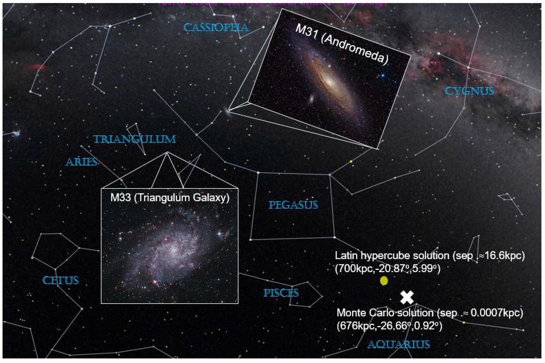
Recently, we checked our Monte Carlo FORTRAN results (reference [21]) using an independent implementation in C++ with a Latin Hypercube9 (LHC) algorithm [33] in order to speed up the time it takes to achieve convergence. The C++ implementation was executed in such a manner as to iteratively improve the LHC lattice spacing until a solution appeared to be converging on the same convergence identified using the FORTRAN code. Figure 7 uses the Satellite Orbital Analysis Program (SOAP) version 14.0.7, from The Aerospace Corporation [34], to plot the location of the CNO center from the LHC and Monte Carlo FORTRAN implementations, showing that it is in the constellation Aquarius.
The separation distance between the extrapolated spin axes for M31 and M33 was 16.6 kiloparsecs from the LHC implementation while the FORTRAN Monte Carlo identified a solution with only a separation of 0.0007 kiloparsecs between the spin axes at a distance of 676 kiloparsecs from the earth with a right ascension of −26.66° and a declination of 0.92°. In the iterative process of reducing the LHC grid spacing we observed the LHC data point in SOAP approaching the Monte Carlo solution on the line from M31 and M33. When this was observed we discontinued using the LHC code, considering the two solutions to be in agreement. Table 7 (also found in [21]10) shows our CNO center results.
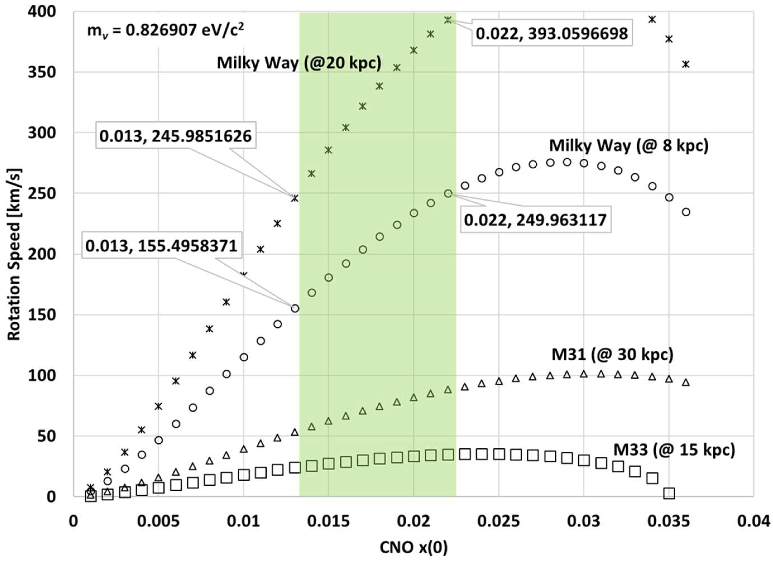
Literature-identified M31, M33 and Milky Way galactic rotation speed data is provided in Table 8: Listed are the distances out from the galactic center to the location in the spiral where approximate low and high-speed rotation values can be obtained from the literature with the identified reference. In addition, Figure 8 graphically shows the vectors used to correlate the CNO’s contribution to the rotation speed for the distances from the galactic center found in the literature.
The virial velocity contribution from the CNO was determined using Equation (7), where the mass at the location from the center (R1) and the mass at the center (RC) were computed by integrating our degenerate neutrino density solutions for various potential degenerate neutrino masses with CNO central Fermi momentum boundary conditions from the CNO center in Equation (8) out to these specific (R1 and RC) distances11.
Figure 9 provides an example of plots used to identify acceptable local group galactic speed solutions (y-axis) for a CNO (in this case with a degenerate neutrino mass of 0.826907 eV/c2) for various central boundary condition values for the Fermi momentum ratio x(0) = (x-axis). Galactic speed constraints from the scientific literature for the Milky Way at 8 and 20 Kilo-parsec (kpc) were used to define the greyed-out area of acceptable Fermi momentum ratio solutions.
This approach leads to the rotational velocity values shown in Table 9, and is a revision to the approach used in [21] (which was to select a Fermi momentum constraint that maximized the M33 rotational speed’s contribution from the CNO for the degenerate neutrino mass best fit value in that paper) to determine our local group CNO’s mass and radius. While not in perfect agreement, these values are not that far off from what was reported in the literature for these spirals at these distances from their galactic centers. That value and our newly determined set of acceptable solutions are plotted in Figure 10 and the 3D local group CNO solution is displayed in Figure 11.
8. Discussion
The question of neutrino condensation is really independent of a cosmological model, as long as a Big Bang scenario is adopted that results in a turbulent primordial plasma, allowing almost unlimited numbers of primordial neutrinos and anti-neutrinos to be produced. Condensed Neutrino Objects would exist by the properties of the elementary particles themselves, and would not depend on a particular cosmology. That said, such objects would have observational signatures.
The available weak lensing data (gravitational bending of light), coupled with the cosmological flat-field curvature result, allows comparison of CNO EOS fits to Dark Matter galaxy cluster data. The degenerate neutrino mass is predicted to be in the 0.8 eV/c2 range. This value can be tested in the upcoming KATRIN measurement [17] of the electron anti-neutrino in beta-decay.
Our CNO density data fits to the Einasto density profile leads to a shape parameter that is an order of magnitude greater than what is reported in the literature [23]. We attribute this difference to the modeling community assumption that Dark Matter must have an EOS of an ideal gas.
It should be pointed out that this value of neutrino mass is supposedly ruled out by Planck satellite data [38]. The problem with the Planck data is that the scientific consortium reducing the raw data assumes that neutrinos and anti-neutrinos are in thermodynamic equilibrium with baryonic matter right up to a de-coupling temperature of ~1 Mega-electron Volts (MeV) [39]. If, in fact, neutrinos radiate power from the mechanism of dipole radiation in turbulent, time-dependent Early Universe magnetic fields, then neutrinos (and anti-neutrinos) are never in thermodynamic equilibrium with baryonic matter, contradicting the key assumption used in reducing the Planck satellite raw data. In place of neutrino degrees of freedom, the reducers of the cosmic microwave background (CMB) raw data would need to use Early Universe magnetic field degrees-of-freedom. This would change their value of the Hubble constant and other derived CMB parameters.
Author Contributions
Each author contributed equally to this research.
Conflicts of Interest
The authors declare no conflict of interest.
References
- Einstein, A. Über den Einfluß der Schwerkraft auf die Ausbreitung des Lichtes. Ann. Phys. 1911, 340, 898–908. (In Germany) [Google Scholar] [CrossRef]
- Einstein, A. Die Grundlage der allgemeinen Relativitätstheorie. Ann. Phys. 1916, 49, 769–822. (In Germany) [Google Scholar] [CrossRef]
- Einstein, A. Kosmologische Betrachtungen zur allgemeinen Relativitätstheorie. Sitzungsberichte der Königlich Preussischen Akad. d. Wissenschaften (Berlin) 1917, 1, 142–152. (In Germany) [Google Scholar]
- Wilkinson Microwave Anisotropy Prob. Available online: https://en.wikipedia.org/wiki/Wilkinson_Microwave_Anisotropy_Prob (accessed on 20 November 2017).
- Zwicky, F. Die Rotverschiebung von extragalaktischen Nebeln. Helv. Phys. Acta 1933, 6, 110–127. (In Germany) [Google Scholar]
- Kitching, T.D.; Rhodes, J.; Heymans, C.; Massey, R.; Liu, Q.; Cobzarenco, M.; Cragin, B.L.; Hassaine, A.; Kirkby, D.; Lok, E.J.; et al. Image Analysis for Cosmology: Shape Measurement Challenge Review & Results from the Mapping Dark Matter Challenge. Astron. Comput. 2015, 10, 9–21. [Google Scholar]
- Kahlhoefer, F. Review of LHC Dark Matter Searches. Int. J. Mod. Phys. A 2017, 32, 1730006. [Google Scholar] [CrossRef]
- López-Corredoira, M. Tests and Problems of the Standard Model in Cosmology. Found. Phys. 2017, 47, 711–768. [Google Scholar] [CrossRef]
- Roos, M. Dark Matter: The evidence from astronomy, astrophysics and cosmology. arXiv, 2010; arXiv:1001.0316. [Google Scholar]
- Lukovic, V.; Cabella, P.; Vittorio, N. Dark matter in cosmology. Int. J. Mod. Phys. A 2014, 29, 1443001. [Google Scholar] [CrossRef]
- Particle Data Group. Review of Particle Physics. Chin. Phys. C 2016, 40, 100001. [Google Scholar]
- Morley, P.D.; Buettner, D.J. Instantaneous power radiated from magnetic dipole moments. Astropart. Phys. 2015, 62, 7–11. [Google Scholar] [CrossRef]
- Jackson, J.D. Classical Electrodynamics, 3rd ed.; Wiley: Hoboken, NJ, USA, 1998. [Google Scholar]
- Grasso, D.; Rubinstein, H.R. Magnetic Fields in the Early Universe. Phys. Rep. 2001, 348, 163–266. [Google Scholar] [CrossRef]
- Morley, P.D.; Buettner, D.J. SHM of galaxies embedded within condensed neutrino matter. Int. J. Mod. Phys. D 2015, 24, 1550004. [Google Scholar] [CrossRef]
- Milky Way. Available online: https://en.wikipedia.org/wiki/Milky_Way (accessed on 20 November 2017).
- KATRIN. Available online: https://www.katrin.kit.edu/ (accessed on 20 November 2017).
- GERDA Collaboration. Background-free search for neutrinoless double-β decay of 76Ge with GERDA. Nature 2017, 544, 47–52. [Google Scholar]
- The Nobel Prize in Physics 2015. Available online: https://www.nobelprize.org/nobel_prizes/physics/laureates/2015/ (accessed on 20 November 2017).
- Morley, P.D.; Buettner, D.J. A dark matter signature for condensed neutrinos. Int. J. Mod. Phys. D 2016, 25, 1650089. [Google Scholar] [CrossRef]
- Morley, P.D.; Buettner, D.J. Dark matter in the local group of galaxies. Int. J. Mod. Phys. D 2017, 26, 1750069. [Google Scholar] [CrossRef]
- Sereno, M.; Fedeli, C.; Moscardini, L. Comparison of weak lensing by NFW and Einasto halos and systematic errors. J. Cosmol. Astropart. Phys. 2016, 2016, 042. [Google Scholar] [CrossRef]
- Retana-Montenegro, E.; Frutos-Alfaro, F. The lensing properties of the Einasto profile. arXiv, 2011; arXiv:1108.4905v1 [astro-ph.CO]. [Google Scholar]
- Gavazzi, R. Projection effects in cluster mass estimates: The case of MS2137-23. Astron. Astrophys. 2005, 443, 793–804. [Google Scholar] [CrossRef]
- Gavazzi, R.; Adami, C.; Durret, F.; Cuillandre, J.-C.; Ilbert, O.; Mazure, A.; Pelló, R.; Ulmer, M.P. A weak lensing study of the Coma cluster. Astron. Astrophys. 2009, 498, L33–L36. [Google Scholar] [CrossRef]
- Irgens, R.J.; Lilje, P.B.; Dahle, H.; Maddox, S.J. Weak Gravitational Lensing by a Sample of X-ray-luminous Clusters of Galaxies. II. Comparison with Virial Masses. Astrophys. J. 2002, 579, 227–235. [Google Scholar] [CrossRef]
- Coe, D.; Umetsu, K.; Zitrin, A.; Donahue, M.; Medezinski, E.; Postman, M.; Carrasco, M.; Anguita, T.; Geller, M.J.; Rineset, K.J.; et al. Clash: Precise New Constraints on the Mass Profile of the Galaxy Cluster A2261. Astrophys. J. 2012, 757, 22. [Google Scholar] [CrossRef]
- Umetsu, K.; Broadhurst, T.; Zitrin, A.; Medezinski, E.; Hsu, L. Cluster Mass Profiles from a Bayexian Analysis of Weak-Lensing Distortion and Magnificantion Measurements: Applications to Subaru Data. Astrophys. J. 2011, 729, 127. [Google Scholar] [CrossRef]
- Anderson, T.W.; Darling, D.A. A Test of Goodness of Fit. J. Am. Stat. Assoc. 1954, 49, 765–769. [Google Scholar] [CrossRef]
- Choulakian, V.; Lockhart, R.A.; Stephens, M.A. Cramér-von Mises Statistics for Discrete Distributions. Can. J. Stat. 1994, 22, 125–137. [Google Scholar] [CrossRef]
- Massey, F.J., Jr. The Kolmogorov-Smirnov Test for Goodness of Fit. J. Am. Stat. Assoc. 1951, 46, 68–78. [Google Scholar] [CrossRef]
- Pearson’s chi-squared test. Available online: https://en.wikipedia.org/wiki/Pearson%27s_chi-squared_test (accessed on 20 November 2017).
- Burkardt, J. IHS—Improved Distributed Hypercube Sampling. Available online: https://people.sc.fsu.edu/~jburkardt/cpp_src/ihs/ihs.html (accessed on 20 November 2017).
- Stodden, D.Y.; Galasso, G.D. Space system visualization and analysis using the Satellite Orbit Analysis Program (SOAP). In Proceedings of the IEEE Aerospace Applications Conference, Aspen, CO, USA, 4–11 February 1995. [Google Scholar]
- Corbelli, E.; Salucci, P. The extended rotation curve and the dark matter halo of M33. Mon. Not. R. Astron. Soc. 2000, 311, 441–447. [Google Scholar] [CrossRef]
- Carignan, C.; Chemin, L.; Huchtmeier, W.K.; Lockman, F.J. The Extended H1 Rotation Curve and Mass Distribution of M31. Astrophys. J. 2006, 641, L109–L112. [Google Scholar] [CrossRef]
- Xin, X.; Zheng, X. A Revised Rotation Curve of the Milky Way with Maser Astrometry. Res. Astron. Astrophys. 2013, 13, 849–861. [Google Scholar] [CrossRef]
- Ade1, P.A.R.; Aghanim, N.; Arnaud, M.; Ashdown, M.; Aumont, J.; Baccigalupi, C.; Banday, A.J.; Barreiro, R.B.; Bartlett, J.G.; Bartolo, N.; et al. Planck 2015 results XIII. Cosmological parameters. Astron. Astrophys. 2016, 594, A13. [Google Scholar]
- Neutrino decoupling. Available online: https://en.wikipedia.org/wiki/Neutrino_decoupling (accessed on 20 November 2017).
- Heavens, A.; Fantaye, Y.; Sellentin, E.; Eggers, H.; Hosenie, Z.; Kroon, S.; Mootoovaloo, A. No Evidence for Extensions to the Standard Cosmological Model. Phys. Rev. Lett. 2017, 119, 101301. [Google Scholar] [CrossRef] [PubMed]
| 1 | The authors performed a rough order of magnitude calculation on the number of expected CNOs in [11]. |
| 2 | v is the neutrino speed, c is the speed of light. |
| 3 | MRI (magnetic resonance imaging) uses this radiation physics. |
| 4 | |
| 5 | eV/c2 is electron Volts divided by the speed of light squared. |
| 6 | The authors are aware of efforts to use lensing of the Cosmic Microwave Background for mapping Dark Matter distributions (https://arxiv.org/pdf/1707.09369.pdf). However, we are awaiting appropriate data to include in future analysis. |
| 7 | For a definition of M200, R200, Mvir and Rvir. please see https://en.wikipedia.org/wiki/Virial_mass. |
| 8 | Coordinates obtained from Wolfram Research’s Mathematica® 11.2. |
| 9 | See for example https://en.wikipedia.org/wiki/Latin_hypercube_sampling for a description of Latin hypercube sampling. |
| 10 | |
| 11 | The rotation speed of a spiral arm is relative to the spiral galaxy’s center. |
Figure 1.
Majorana neutrinoless double beta decay4, not seen experimentally.
Figure 1.
Majorana neutrinoless double beta decay4, not seen experimentally.
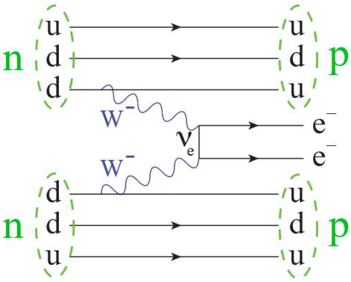
Figure 2.
Neutrino flavor mixing for condensed neutrinos.

Figure 3.
The figure shows the mass density (ρ) per solar mass per Kilo-parsec (kpc) cubed against the CNO radius in Mega-parsecs (Mpc) for a degenerate neutrino mass of 0.8 eV/c2 for central x(0) boundary conditions ranging from 0.005 to 0.01 with overlaid Einasto density model fits as: (a) linear-linear plot; (b) log-log plot.

Figure 4.
The plotted virial mass and radii from identified weak lensing data.
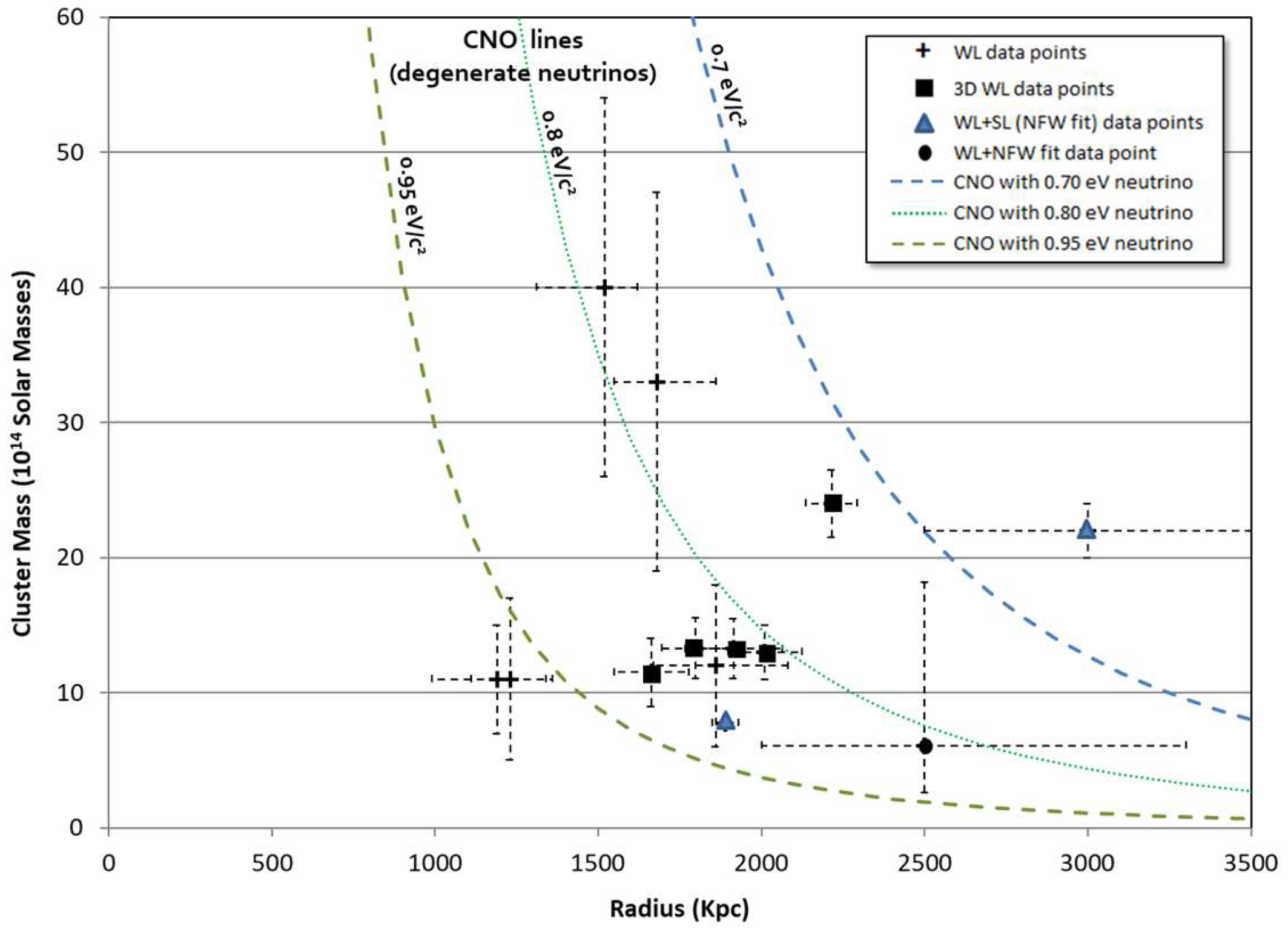
Figure 5.
The log-log plotted virial mass and radii from identified weak lensing data with best fit to the data (0.827 eV/c2) line and the 95% Confidence Interval lines of ±0.059 eV/c2 from the best fit line, respectively.
Figure 5.
The log-log plotted virial mass and radii from identified weak lensing data with best fit to the data (0.827 eV/c2) line and the 95% Confidence Interval lines of ±0.059 eV/c2 from the best fit line, respectively.
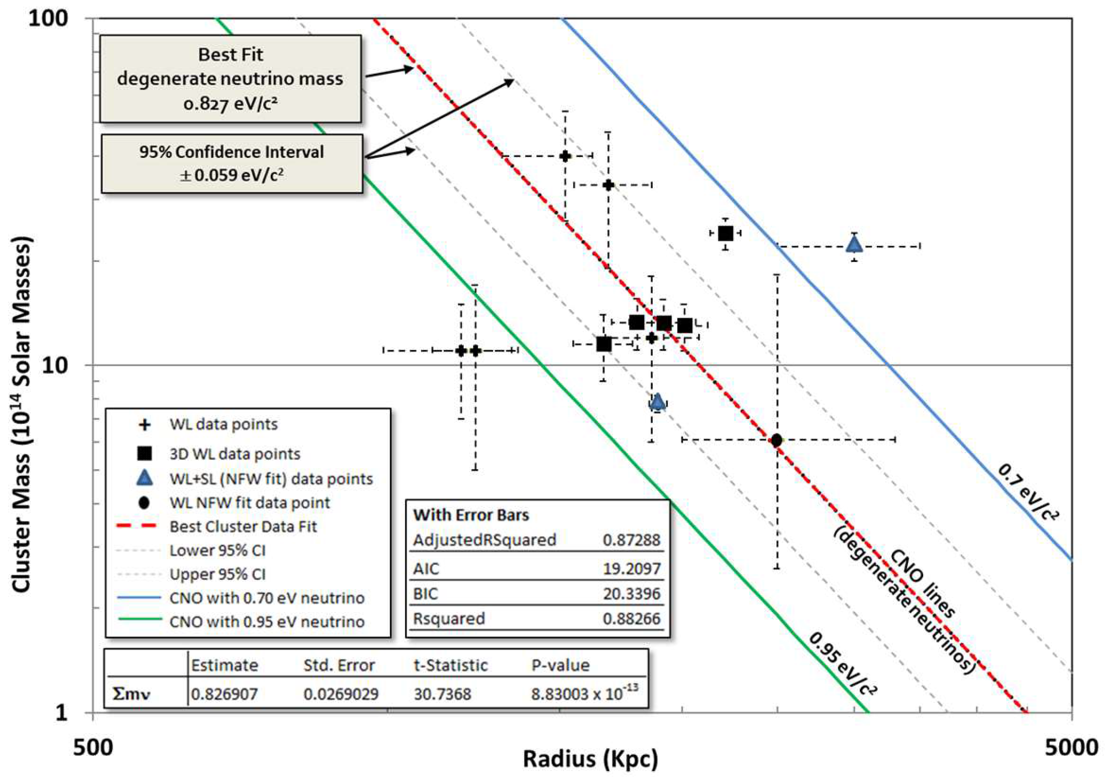
Figure 6.
Our Local Group CNO spiral galaxy orientation. Two of the three embedded spiral galaxies have spin axis which are radially aligned to the CNO center, while the Milky Way has a canted spin axis from the center.
Figure 6.
Our Local Group CNO spiral galaxy orientation. Two of the three embedded spiral galaxies have spin axis which are radially aligned to the CNO center, while the Milky Way has a canted spin axis from the center.
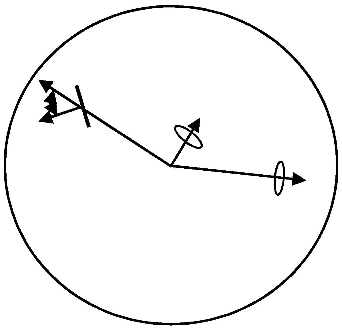
Figure 7.
The local group’s CNO center plotted using The Aerospace Corporation’s SOAP version 14.0.7 as determined by independent implementations in C++ and FORTRAN.
Figure 7.
The local group’s CNO center plotted using The Aerospace Corporation’s SOAP version 14.0.7 as determined by independent implementations in C++ and FORTRAN.

Figure 8.
The geometry for the CNO’s center to distances from the center of the galaxies was used for computing the density differences for: (a) the canted Milky Way’s center to 8 kilo parsecs out from the center using the law of cosines; (b) the simpler geometry for M31 from the center to 15 kilo parsecs out with no cant angle.

Figure 9.
Plots potential local group spiral galactic speed solutions (y-axis) for a CNO for a degenerate neutrino mass of 0.826907 eV/c2 against various central boundary condition values for the Fermi momentum ratio (x-axis).
Figure 9.
Plots potential local group spiral galactic speed solutions (y-axis) for a CNO for a degenerate neutrino mass of 0.826907 eV/c2 against various central boundary condition values for the Fermi momentum ratio (x-axis).

Figure 10.
The plotted virial mass and radii from identified weak lensing data now also displaying acceptable Local Group CNO solutions, including the CNO mass and radii values used in Figure 11.
Figure 10.
The plotted virial mass and radii from identified weak lensing data now also displaying acceptable Local Group CNO solutions, including the CNO mass and radii values used in Figure 11.

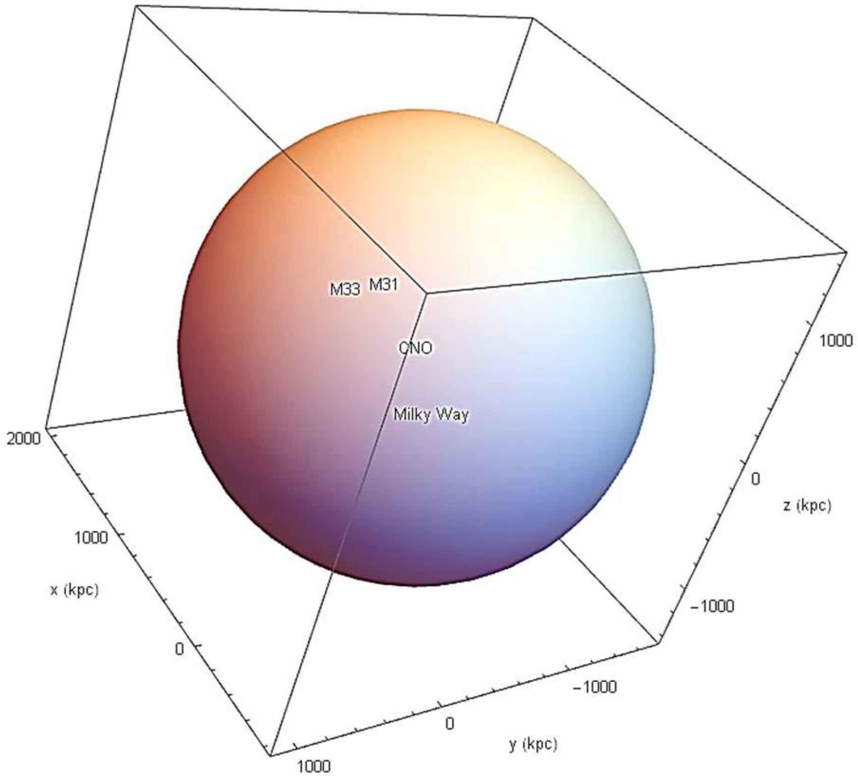
Figure 11.
Plots the FORTRAN 3D solution bounding CNO with the locations of M31, M33 and the Milky Way.
Figure 11.
Plots the FORTRAN 3D solution bounding CNO with the locations of M31, M33 and the Milky Way.


Table 1.
Hydrostatic solutions for degenerate neutrino matter.
| x(0) (for mνc2 = 1 eV) | Mtotal (MΘ) | R0 (ly) | Ω (joules) | R0 (RS) |
|---|---|---|---|---|
| 0.001 | 3.100 × 10¹³ | 13.01 × 10⁶ | −1.764 × 1054 | 1.344 × 10⁶ |
| 0.01 | 9.809 × 10¹⁴ | 4.12 × 10⁶ | −5.569 × 1057 | 1.345 × 10⁴ |
| 0.1 | 3.077 × 10¹⁶ | 1.30 × 10⁶ | −1.739 × 1061 | 135.3 |
| 1.0 | 5.27 × 10¹⁷ | 3.72 × 10⁵ | −1.969 × 1064 | 2.254 |
Note. x(0) is the Fermi momentum, MΘ is the solar mass, R0 is the radius, ly is light years, Rs is the Schwarzschild radius.
Table 2.
Interesting CNO properties.
| Interesting Property | Consequence |
|---|---|
| CNO obey Pauli Exclusion Principle | CNO cannot grow from fusion (like Black Holes)—CNO repel each other |
| Embedded matter (galaxies and gas) undergo simple harmonic motion | Embedded gas is not in thermodynamic equilibrium, contrary to assumptions in x-ray data analysis |
| CNO can be internally excited (lowest excited state is a quadrupole oscillation) | CNO do not necessarily have a spherical shape |
| CNO are primarily composed of the original cosmological neutrinos and anti-neutrinos formed in the Big Bang | CNO are common objects (not rare) |
Table 3.
Einasto density fit parameters for three cases of degenerate neutrino masses.
| Spherical CNO Properties | Einasto Density Parameters | |||||
|---|---|---|---|---|---|---|
| mν (eV/c2) | x(0) | M(Rmax) (1014 Mo) | Rmax (Kpc) | ρ−2 (per Mo/Kpc3) | r−2 (Kpc) | α |
| 0.7 | 0.005 | 7.07563 | 3646.02 | 8336.41 | 1853.96 | 2.2081 |
| 0.006 | 9.30115 | 3329 | 14,409.6 | 1692.09 | 2.20887 | |
| 0.007 | 11.7211 | 3082.04 | 22,878.5 | 1566.69 | 2.20832 | |
| 0.008 | 14.3206 | 2883.2 | 34,148.4 | 1465.54 | 2.20801 | |
| 0.009 | 17.0877 | 2718.57 | 48,638.3 | 1381.42 | 2.20893 | |
| 0.01 | 20.0131 | 2579.16 | 66,700.5 | 1310.7 | 2.20801 | |
| 0.015 | 37.4921 | 2107 | 22,5235 | 1069.76 | 2.20918 | |
| 0.02 | 56.5911 | 1823.84 | 533,578 | 926.671 | 2.20704 | |
| 0.8 | 0.005 | 5.41728 | 2794 | 14,219.9 | 1419.48 | 2.20743 |
| 0.006 | 7.12107 | 2550 | 24,564.9 | 1295.97 | 2.20644 | |
| 0.007 | 8.97393 | 2360 | 39,046.8 | 1199.14 | 2.20924 | |
| 0.008 | 10.9657 | 2208 | 58,287.6 | 1121.65 | 2.20922 | |
| 0.009 | 13.0828 | 2081.46 | 82,932 | 1057.9 | 2.20699 | |
| 0.01 | 15.3225 | 1974.72 | 113,784 | 1003.47 | 2.20745 | |
| 0.015 | 28.1461 | 1612.37 | 384,147 | 819.097 | 2.20792 | |
| 0.02 | 73.6874 | 1397 | 909,020 | 709.983 | 2.20246 | |
| 0.95 | 0.005 | 3.84162 | 1983 | 28,278.5 | 1006.5 | 2.20706 |
| 0.006 | 5.04993 | 1808 | 48,899.8 | 918.405 | 2.20894 | |
| 0.007 | 7.27676 | 1674 | 77,601.6 | 850.565 | 2.20691 | |
| 0.008 | 7.77518 | 1565.37 | 115,867 | 795.492 | 2.20753 | |
| 0.009 | 9.42287 | 1477 | 164,901 | 750.167 | 2.20606 | |
| 0.01 | 10.9897 | 1401 | 226,441 | 711.225 | 2.209 | |
| 0.015 | 19.9595 | 1143.38 | 762,388 | 581.445 | 2.2013 | |
| 0.02 | 31.1658 | 990.5 | 1,807,020 | 503.513 | 2.20053 | |
Table 4.
Identified weak lensing data and two data points from weak lensing and strong lensing data which used an NFW density fit.
Table 4.
Identified weak lensing data and two data points from weak lensing and strong lensing data which used an NFW density fit.
| Cluster | z | Mvir (1014 Mo) | Rvir (Mpc) | Type | Reference |
|---|---|---|---|---|---|
| MS2137-23 * | 0.310 | 1.89 ± 0.04 | SL+WL (NFW fit) | [24] | |
| Coma (Abell 1656) ** | 0.024 | WL NFW | [25] | ||
| A914 | 0.193 | 11 ± 6 | WL | [26] | |
| A1351 | 0.328 | 33 ± 14 | WL | [26] | |
| A1576 | 0.299 | 40 ± 14 | WL | [26] | |
| A1722 | 0.326 | 12 ± 6 | WL | [26] | |
| A1995 | 0.321 | 11 ± 4 | WL | [26] | |
| A2261 | 0.225 | 22 ± 2 | ~3 | SL+WL (NFW fit) | [27] |
| A1689 | 0.183 | 13 ± 2.05 | 2.011 ± 0.113 | 3D WL | [28] |
| A1703 | 0.281 | 13.25 ± 2.21 | 1.915 ± 0.148 | 3D WL | [28] |
| A370 | 0.375 | 23.99 ± 2.49 | 2.215 ± 0.079 | 3D WL | [28] |
| Cl0024 + 17 | 0.395 | 13.29 ± 2.24 | 1.799 ± 0.105 | 3D WL | [28] |
| RXJ1347 − 11 | 0.451 | 11.5 ± 2.50 | 1.663 ± 0.115 | 3D WL | [28] |
* Uses M200 and R200, thus may be an underestimate of Mvir and Rvir.; ** Uses Rvir at .7
Table 5.
Goodness-of-fit statistics from 5000 Monte Carlo iterations for the five common tests provided by Mathematica®. CI is Confidence Interval; IQR is Interquartile Range.
Table 5.
Goodness-of-fit statistics from 5000 Monte Carlo iterations for the five common tests provided by Mathematica®. CI is Confidence Interval; IQR is Interquartile Range.
| Goodness-of-Fit statistics mν = 0.8269 (5000 Monte Carlo iterations) | Mean p-value | Mean CI | Variance | Median p-value | IQR |
|---|---|---|---|---|---|
| Anderson-Darling [29] | 0.464 | ±0.006 | 0.049 | 0.415 | 0.397 |
| Cramér-von Mises [30] | 0.446 | ±0.006 | 0.048 | 0.379 | 0.384 |
| Kolmogorov-Smirnov [31] | 0.513 | ±0.007 | 0.063 | 0.379 | 0.403 |
| Pearson χ2 [32] | 0.564 | ±0.005 | 0.031 | 0.53 | 0.304 |
| Watson U2 [30] | 0.33 | ±0.006 | 0.041 | 0.261 | 0.313 |
Table 6.
Coordinates of the Local Group spiral galaxies.8
Table 6.
Coordinates of the Local Group spiral galaxies.8
| Name | Distance (kpc) | Dec (°) | RA (°) |
|---|---|---|---|
| M31 | 788.333 | 41.2689 | 10.685 |
| M33 | 862.417 | 30.6581 | 23.466 |
| Milky Way | 7.61113 | −29.0078 | 266.417 |
Table 7.
Monte Carlo-derived CNO Local Group parameters.
| Quantity | Predicted Value |
|---|---|
| Center CNO-LG distance from MW | 673.422 kpc |
| Center CNO-LG distance from M33 | 740.423 kpc |
| Center CNO-LG distance from M31 | 656.015 kpc |
| Algorithm error center CNO-LG | 0.000706162 kpc |
| Right ascension of CNO-LG center | −26.6588° |
| Declination of CNO-LG center | 0.91773° |
| Galactic longitude of CNO-LG center | 62.83928785° |
| Galactic latitude of CNO-LG center | −42.77834848° |
| Milky way cant angle | 47.221° |
Table 8.
Local Group Approximate Rotational Speed Values from the Galactic Center.
| Local Group Galaxy | Distance from Center (kpc) | VDM Low (km/s) | VDM High (km/s) | Reference |
|---|---|---|---|---|
| M33 | 15 | ~65 | ~110 | [35] |
| M31 | 30 | ~50 | ~110 | [36] |
| Milky Way | 8 | ~80 | ~260 | [37] |
| Milky Way | 20 | ~250 | ~400 | [37] |
Table 9.
Local Group CNO-induced approximate galactic rotational speeds for the degenerate neutrino masses determined from the weak lensing data fits.
Table 9.
Local Group CNO-induced approximate galactic rotational speeds for the degenerate neutrino masses determined from the weak lensing data fits.
| 0.768290 eV/c2 | 0.826907 eV/c2 | 0.88552 eV/c2 | |||||||
|---|---|---|---|---|---|---|---|---|---|
| x(0) boundary values → | 0.014 | 0.017 | 0.021 | 0.013 | 0.017 | 0.022 | 0.013 | 0.019 | 0.025 |
| M33 (@ 15 kpc) (km/s) | 26 | 31 | 38 | 24 | 30 | 35 | 23 | 27 | 16 |
| M31 (@ 30 kpc) (km/s) | 56 | 70 | 88 | 54 | 71 | 88 | 54 | 73 | 76 |
| MW (@ 8 kpc) (km/s) | 162 | 203 | 253 | 155 | 204 | 250 | 156 | 203 | 201 |
| MW (@ 20 kpc) (km/s) | 257 | 321 | 399 | 246 | 322 | 393 | 246 | 319 | 310 |
© 2017 by the authors. Licensee MDPI, Basel, Switzerland. This article is an open access article distributed under the terms and conditions of the Creative Commons Attribution (CC BY) license (http://creativecommons.org/licenses/by/4.0/).
Share and Cite
MDPI and ACS Style
Morley, P.; Buettner, D. Weak Lensing Data and Condensed Neutrino Objects. Universe 2017, 3, 81. https://doi.org/10.3390/universe3040081
AMA Style
Morley P, Buettner D. Weak Lensing Data and Condensed Neutrino Objects. Universe. 2017; 3(4):81. https://doi.org/10.3390/universe3040081
Chicago/Turabian StyleMorley, Peter, and Douglas Buettner. 2017. "Weak Lensing Data and Condensed Neutrino Objects" Universe 3, no. 4: 81. https://doi.org/10.3390/universe3040081
Note that from the first issue of 2016, this journal uses article numbers instead of page numbers. See further details here.