1. Introduction
Novel behaviours for electromagnetic rays result from the combination of gravitational lensing and the optical effects from a dispersive plasma medium [
1,
2]. The joint effects of gravitation, refraction and dispersion have been studied using homogenous [
3,
4] and inhomogenous plasma distributions [
5] on a variety of scales [
6,
7] and geometries [
8,
9,
10]. Bound orbits of rays under the effect of gravity and plasma have also been discussed [
5,
11]. The effect of a power-law distribution of transparent plasma on the pulse profiles of a compact object (CO) have been shown to produce frequency-dependent shifts [
12], and trapping of rays [
13].
In the environment of a highly luminous neutron star (NS), a distribution of plasma is strongly affected by both radiation pressure and gravity [
14,
15,
16]. In the Newtonian picture, the radiative force decreases as
, and therefore if radiation overpowers gravity at a particular radius it is true for all space. However, the situation described by general relativity is more subtle. In Schwarzschild space-time the radiative force changes at a faster rate than gravitational effects [
17,
18]. Thus, there is only a single radius at which the effects of gravity and radiation on a test particle are balanced. This position of radial equilibrium defines a surface called the Eddington capture sphere (ECS [
17,
19]). At this radius, a stable shell of plasma can collect, detached from the NS surface [
20]. These levitating atmospheric shells have been studied in optically thin and optically thick conditions [
21,
22].
In this work, we assume that the optically thin levitating atmosphere around a CO can be treated as a transparent plasma shell and that radiation is free to propagate between the stellar surface and the shell. We calculate the resulting frequency-dependent ray trajectories under the effects of gravitation from the CO as well as refraction and dispersion from the plasma shell. In
Section 2 we discuss the theoretical aspects of levitating atmospheres and the ray-tracing procedure. In
Section 3 we present our numerical results.
Section 4 provides discussion of our calculations and the general results that we have obtained, as well as example density functions. Finally, we summarize our findings in
Section 5.
2. Theory
Let us use the set of units in which
. We assume spherical symmetry, and without loss of generality work in the equatorial plane
. The Schwarzschild line element is
with
As a first approach, let us treat the plasma shell as a non-magnetized, inhomogenous optically-thin medium with index of refraction of the form
with ray frequency
ω and local plasma frequency
where the plasma particles have charge
q and mass
m, and
describes the number density distribution of the plasma, scaled by the maximum
. On the right hand side we have consolidated the coefficients into the constant
k. For the remainder of our numerical work we use a simple exponential function to describe the shell density
with the maximum located at a distance
, where
R is the radius of the CO. Despite these assumptions, our conclusions will be general, and will not depend on the exact details of the density function. The numerical examples in the body of the text use Equation (
5), however we consider other density functions in
Section 4. In fact, any shell-like density profile will generate qualitatively similar results. Throughout the text we will refer to the plasma density as
N, and suppress the radial dependence for simplicity.
The Hamiltonian for an electromagnetic ray under the effect of gravity and an optical medium was first considered by Synge [
23]. This result was subsequently specialized to non-homogenous plasma [
2,
3], which we state using Equations (
3)–(
5),
The equations of motion are
and
The derivatives of the
t and
ϕ momenta vanish, providing the constants of motion
where
is the ray frequency an observer at infinity would detect provided the ray escapes, and
where
L is the angular momentum. Since we restrict the trajectories to the equatorial plane, the momentum
vanishes. With this restriction the indices
i,
j and
k each take the values
t,
r and
ϕ. For a static medium the effective redshift relationship is given by
The corresponding coordinate derivatives are
For spherical symmetry, there is no orbital motion out of the
plane. The radial momentum is given by Equation (
6) vanishing,
with the sign of
denoting a radially infalling ray as
and an outgoing ray with
. The derivative of the radial momentum is
giving the radial coordinate derivative
Finally, we find the change in angle as a function of radius using Equations (
13), (
14) and (
16),
The effective potential that includes the effect of the plasma is
with first and second derivatives
These general expressions with power-law density reproduce the corresponding equations from [
12]. Circular orbits are found at radial distances where the derivative of the effective potential vanishes [
24,
25]. We call these extremal radii
, where
e takes the labels
s for a stable orbit and
u for an unstable orbit. Stable minima further require
Solving for the corresponding
L with
gives the angular momentum required to produce a circular orbit
with
.
Levitating spherical shell-type atmospheres around COs are physically motivated and have an established theoretical foundation in the literature [
14,
22]. To explore the basics of these solutions, let us follow the approach in [
21] and write the observed stellar luminosity as
. Then the local stellar luminosity as a function of radial distance
r from the CO is given by
The observed Eddington luminosity is
where
m is the plasma particle mass and
is the cross-section for Thomson scattering. However, the Eddington luminosity can also be used to define a local critical luminosity required to produce a radiative force which balances gravity at a distance
r [
15]. The local critical luminosity is
The radius at which the stellar luminosity
ℓ is equal to the critical luminosity
defines a spherical surface around the CO called the Eddington capture sphere [
15,
21] with radius
where the ratio of the observed luminosity and the Eddington luminosity is
Plasma particles near the CO are subject to radiation drag and have their angular momentum reduced [
26]. These particles gather on the ECS since it is an equilibrium position in the radial direction [
17,
19] and is stable against radial oscillations [
20].
The stability of the ECS allows for the formation of a levitating shell of plasma. For larger values of the luminosity ratio,
, these levitating atmospheres are separated from the NS surface with no significant density between. Analytical density profiles have been constructed for isothermal and polytropic levitating atmospheres in the optically thin case [
21]. The polytropic atmospheres have thickness that depends on the temperature
T, with higher
T producing more distended atmospheres. The optically thick case has also been investigated numerically [
22]. The radiative equilibrium condition has been used in the analysis of photospheric expansion X-ray bursts from NSs [
27,
28,
29,
30], and the effect of a levitating atmosphere may also contribute to the nature of these bursts [
21,
26].
Our assumed density
N (Equation (
5)) approximates the rapid drop-off from the peak density
of the levitating polytropic fluid shells [
21] while remaining analytically simple. However, our conclusions are qualitatively insensitive to the particulars of
N, provided a maximum external to the stellar surface. Thus, we are not concerned with the exact details that lead to the levitating atmosphere solution and rather seek to capture the general character of these plasma shells in our numerical examples.
We will examine the trajectories of electromagnetic rays by ray-tracing. We assume a ray of energy
E and angular momentum
L begins at an initial position
, directed inward or outward depending on the choice of sign for
. We then solve Equations (
9)–(
16) numerically to find the path of the ray under the influence of gravity and the effect of the plasma given by the density
N in Equation (
5). The integration of the equations of motion is ceased when the trajectory intersects the stellar surface or escapes to a significant distance (
). For bound rays, we follow the orbits for an arbitrary number of time-steps, chosen to give a few periastron-apastron pairs.
3. Numerical Results: A Variety of Novel Orbits
To initialize our numerical ray-tracing routine, we select the physical parameters that describe our CO and the levitating atmospheric shell. We choose the mass of the CO as
. To maximize the gravitational effects, we use an extremely relativistic compactness ratio of
, at the stiff end of the nuclear EoS [
13,
31]. We choose a relatively high ratio of stellar to Eddington luminosity of
, which gives the center of the shell at
. Finally, we estimate the thickness of the shell using the approximate formula from [
21,
which gives
km for our choices of parameters. We then set
and
in our test function, given in Equation (
5).
The equations of motion show us that the constant
k sets the frequency at which plasma effects become relevant to the ray trajectories, but the dynamics of the rays are unchanged provided we redefine the momenta
, as well as the affine parameter
. Thus, in our numerical examples we simply set
and discuss the relevant frequency scale in
Section 4.
3.1. A Stable Circular Orbit for Electromagnetic Rays
When an optically thin levitating atmosphere with a refractive index is considered, the effective potential is significantly more complicated than the vacuum case and allows for a variety of circular orbits. As a numerical example, let us consider a ray that has a frequency . Such a ray with angular momentum has a stable circular orbit at . This stable circular orbit is well within the radius of the ECS, . The unstable circular orbit radius for electromagnetic rays at the potential maximum, , is shifted inward slightly from the ECS radius due to the contribution from the angular momentum term in the effective potential.
Generally, any shell-like plasma atmosphere with a density profile
N that has a maximum at
and which is physically realistic (decreases as a function of
r in both directions
and
and which vanishes at infinity) will produce a minimum in the effective potential, resulting in a stable circular orbit. The existence of this stable circular orbit does not require any additional symmetry arguments be imposed on the shell density, provided the previous conditions are satisfied. For example, an asymmetrical density profile was found for an isothermal levitating atmosphere [
21], though this is not a physically realistic solution since the density does not vanish at infinity. However, such a density profile would still produce a stable circular orbit within
.
3.2. Periodic Orbits
Bound ray trajectories admit periodic solutions with the appropriate angular momentum
L for a given energy
E. Consider the time elapsed between the closest distance of the orbit from the central CO, the periastron radius
and the furthest distance, the apastron radius
. Let us define the angle accumulated as the integral of Equation (
17) for a bound orbit,
Using Equation (
17) the right hand side gives
The quantity
is the ratio of the radial and angular frequencies found from the Hamiltonian using action-angle variables [
32],
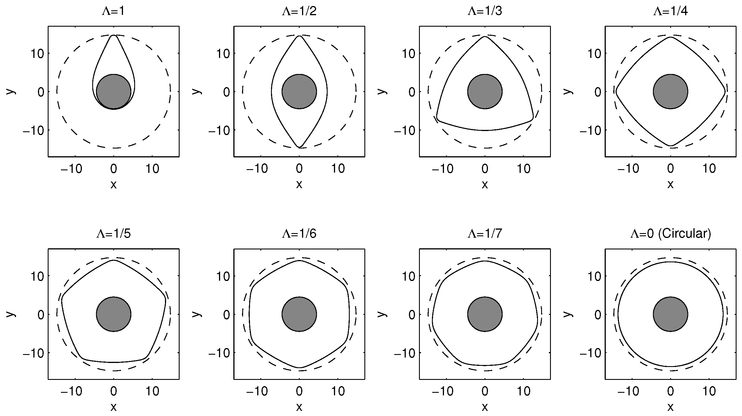
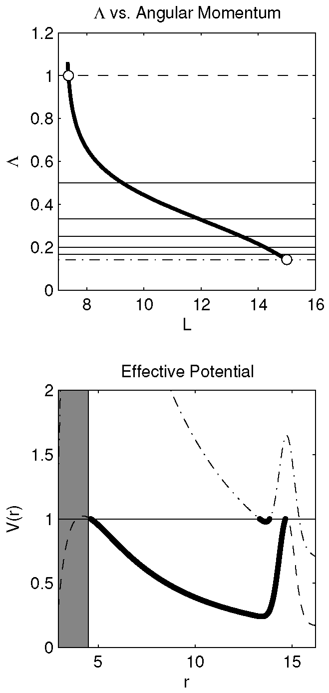
Periodic orbits have a rational value of Λ. In the upper panel of
Figure 1 we calculate Λ as a function of
L, holding
, via Equation (
30). We then numerically find the corresponding values of
L for which Λ equals 1,
,
,
,
,
and
. The stable circular orbit has
. For
(dashed line) and
(dash-dotted line) we plot the corresponding effective potentials in the lower panel, and show the potential experienced by the bound orbit as a thick black line. The ratio Λ is bounded in
L since a bound orbit requires a potential minimum. When
L is too low, no inner (stable) potential boundary exists between
R and
. For
L too high, orbits are not bound by the contribution to the effective potential from the shell. In
Figure 2 we plot the periodic orbits corresponding to these Λ values.
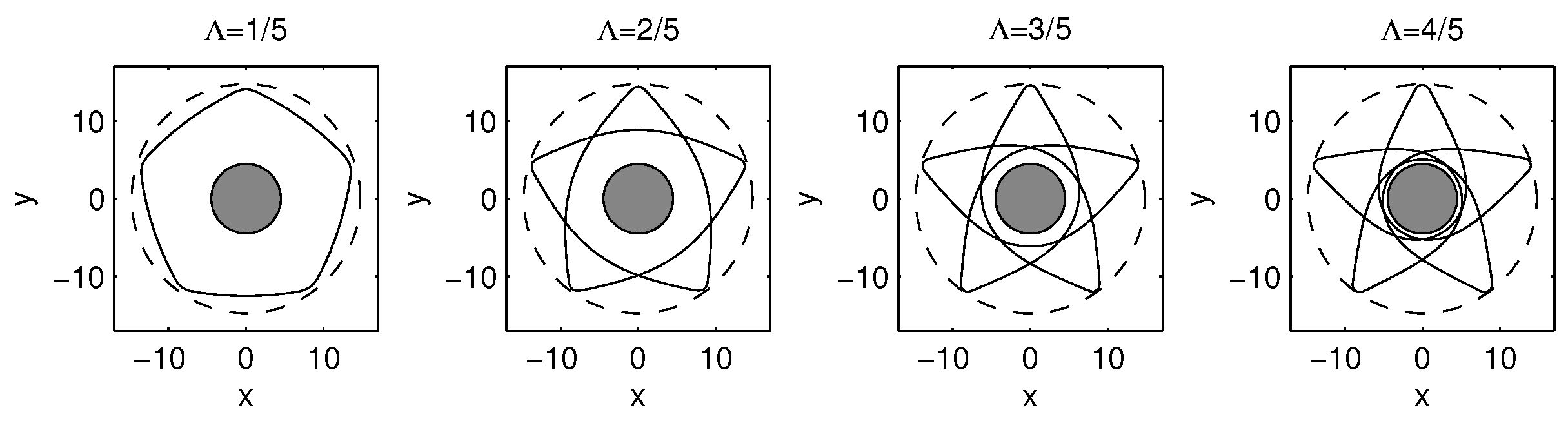
For the periodic orbits the denominator of the rational Λ values denote the number of deflections from the effective potential barrier provided by the plasma in a complete orbit. The numerator describes the complexity of the orbit. For example, let
be a rational number. The resulting orbit has
β reflections off of the plasma shell and the path intersects itself
times. A family of periodic orbits with
,
,
and
is plotted in
Figure 3 to demonstrate. These orbits each contain 5 reflections from the plasma shell and feature 0, 5, 10 and 15 intersections of the orbital path.
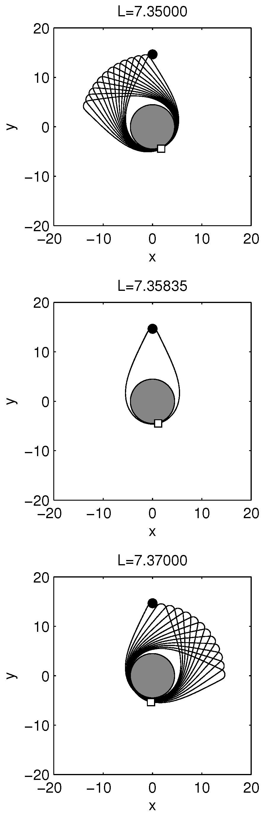
In terms of angular momentum, the periodic configurations are preceded and followed by orbits with similar morphology but which precess in the opposite sense. For example, the
periodic orbit is shown in the center panel of
Figure 4. We integrate the equations of motion until the coordinate time component reaches an arbitrary value sufficient to provide several orbits of the CO. The initial position is marked as a black dot and the final position is a square. Given a periodic orbit with
, a lower angular momentum orbit with
precesses in a counter-clockwise manner (top panel), and an orbit with
precesses in the opposite sense (bottom panel).
3.3. Frequency Windows
We define two particularly significant frequency ranges for rays that interact with the plasma atmosphere. The escape window (EW) is defined by the frequency range
. Rays in this frequency window can escape from the CO surface to reach an observer at infinity, but the trajectories are strongly influenced by the presence of the plasma atmosphere. Below the EW a second frequency band exists,
, which we refer to as the anomalous propagation window (APW). In this frequency range, rays are trapped by the plasma. Rays in the APW that leave the surface of the CO travel to a maximum altitude and then turn back to the CO surface. This trapping is analogous to the anomalous propagation of low-frequency radio waves in the atmosphere of the Earth. In addition to a family of trapped rays emitted from the CO surface, the APW also includes a set of rays that approach the the plasma atmosphere from the outside and are scattered off of it. The EW and APW were explored in [
13] for a CO surrounded by a cloud of plasma with a power-law density.
We define the asymptotic plasma frequency
in analogy with the ray frequency at infinity (Equation (
9)) using the redshift definition (Equation (
11)),
such that the propagation of radiation requires
to exceed
along the path of a ray. In fact, the quantity on the right hand side is simply the square root of the effective potential with
, for which
.
The limiting frequency for a radially directed ray to escape is given by Equation (
32) at
,
The condition on radially directed rays defines the floor of the EW and the APW ceiling. We will focus on each of the frequency ranges separately in the following sections.
3.3.1. Ray Trapping
Outgoing radially-directed rays with
cannot propagate through the plasma atmosphere. Since the effective potential contains a contribution from the angular momentum, turning points exist for all rays with finite
L,
Therefore, provided
, all rays with
are scattered. Rays with finite angular momentum that are emitted from the CO surface reach a maximum height and return to the CO surface. This trapping requires a potential maximum outside the stellar surface,
, and thus we define the lower APW limit as
For incoming rays that approach the CO atmospheric shell externally, we write the angular momentum as
where
b is the impact parameter. For non-vanishing
b, the approaching rays reach a minimum distance before scattering from the plama atmosphere due to the presence of a turning point and return to infinity.
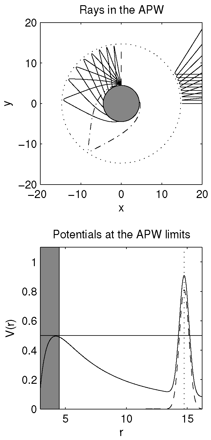
We plot examples of rays in the APW in
Figure 5 and use
, well below the APW ceiling
for the choice of example parameters in our units. We plot the trajectories of ten rays launched from
R at position
. We vary the angular momenta of the rays from 0 (dashed ray) to
(dashed-dotted ray), where the maximum angular momentum is found by setting by relating the square of the frequency and the turning point at the surface,
At and above
, the ray is in a bound orbit and only skims the surface tangentially at
R. The ECS radius is plotted as a dotted circle. External rays that approach from the
direction are scattered by the plasma atmosphere. For these rays we used the same frequency and an identical set of angular momenta, giving the impact parameters
The fiducial ray does not propagate in the plasma since
for the
case. In the bottom panel we plot the effective potential for the
ray (dashed curve) and the potential for a ray with
(solid curve). The horizontal line is
. The interior of the CO is the shaded region and the ECS radius is plotted as the vertical dotted line.
3.3.2. Ray Escape
The angular momentum corresponding to the upper limit of the EW is generally found when
Using the above relationship to find the angular momentum results in
This expression simplifies for the case of a gaussian shell, in which case we realistically assume the extent of the atmosphere is thin and does not significantly contribute at
, and that the ECS is sufficiently far from the stellar surface such that
. With these assumptions Equation (
39) becomes
which gives the asymptotic frequency
Rays with frequencies in the range
can escape the surface of the CO and are detectable by distant observers.
In the vacuum case the maximum impact parameter is given by a ray escaping from an emission point at
R with a launch angle
with respect to the radial direction to arrive at a distant observer. The maximum impact parameter is given by
The maximum impact parameter for a ray in the EW with frequency
differs from the vacuum case due to the presence of the unstable circular orbit, and is found using Equation (
42) with
R replaced by
,
The ray is launched at an angle given by the ratio with the maximum impact parameter,
The maximum impact parameter for a ray in the EW is the solution for which the denominator of Equation (
17) vanishes. Expanding the denominator gives
The minimum of this cubic function occurs at
, and the choice
ensures a single unique solution [
13].
Beyond the EW,
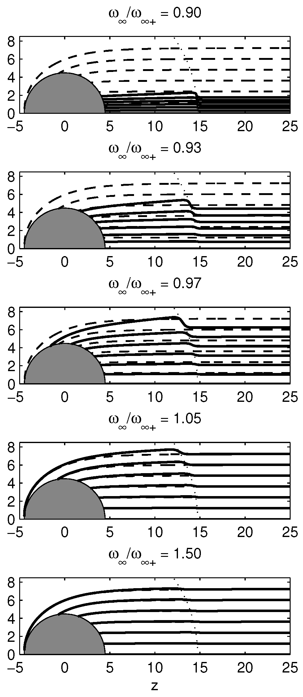
, rays experience trajectory modification between the surface of the CO and the atmospheric plasma shell but approximate the vacuum trajectories at greater distances. As the frequency is increased, the vacuum trajectories are recovered. We show the ray trajectories for a variety of rays within and above the EW in
Figure 6. For our example parameters, we launch rays in the EW from the surface of the CO with the frequency ratio
for values of
,
,
. We also plot the cases for rays above the EW for frequency ratios
and
. The highest frequency ratio appears very similar to the vacuum case.
4. Discussion
Let us estimate the minimum observable frequency
visible to a distant observer. Since this quantity depends on the ratio of stellar to Eddington luminosity, we will estimate an upper limit given by the plasma frequency (Equation (
4)) at the ECS radius. We use the maximum mass density
in the range
to
g·cm
[
22] to estimate the plasma frequency cut-off. Converting from plasma particle mass density to number density gives
where
is the proton mass and
the mean molecular weight. With these values we find
between ∼6 and ∼60 THz, in the mid to near infrared portion of the electromagnetic spectrum. However, since
depends on the value of
λ, this estimate is an upper limit. Moreover, for the choice of
used here, we emphasize the effect of changing the plasma frequency constant
k amounts to a simple re-scaling of the dynamical quantities that enter the equations of motion as discussed in
Section 3.
Other effects may additionally reduce this estimate, for example if the atmospheric plasma particles have a significant velocity spread the Lorentz factor modifies the effective plasma frequency [
33]. Thus, we expect the observed frequency range to be sensitive to the effects of temperature in the atmospheric shell [
21] and strong magnetic fields from the CO (neglected in previous studies). Including these conditions requires a more complex dispersion relation (for examples, see [
34]).
Our results show that while the high frequency radiation receives little modification from the vacuum case, the lower frequency components are dramatically modified, particularly for frequencies in the EW. The behaviour of these rays under the influence of both gravitation and the optical effects introduced by the plasma atmosphere significantly affect the appearance of the CO that a distant observer would measure. This frequency-dependent view alters the observed pulse profile, an effect which has been studied for COs surrounded by a power-law plasma density [
12,
13,
35]. The change in behaviour of the pulse profiles at frequencies in the EW may give an analogous signature of the presence of the optically thin levitating atmospheric shell. With a relatively high plasma frequency such effects may be feasible to observe.
We have considered non-rotating COs and have assumed spherical symmetry. In practice, rotation significantly impacts pulse profiles, particularly through the Doppler effect [
36]. Including the effects of rotation would provide additional modifications to the basic spherically symmetric calculations detailed here.
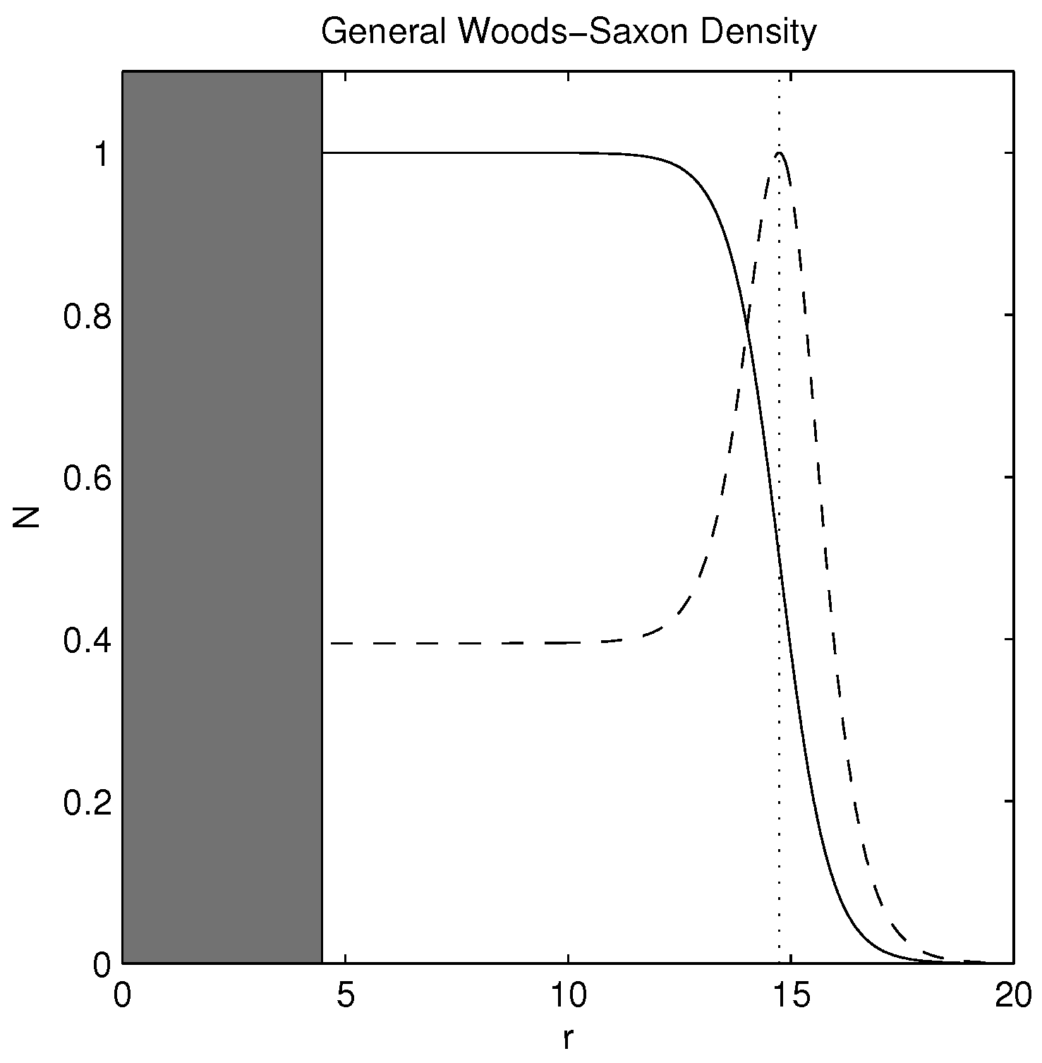
Finally, we demonstrate the generality of our results by considering an extreme case. The gaussian shell density has a well-defined local maximum at
, so it is interesting to consider the resulting trajectories when this assumption does not hold and the shell is thick. We have constructed a density profile based on the form of the generalized Woods-Saxon potential used in modeling nuclear interactions [
37]. The resulting density profile differs significantly from the gaussian shell scenario since the Woods-Saxon type density does not vanish at the stellar surface. Though these cases are not necessarily physically realistic, they provide an interesting test of our results. The Woods-Saxon density is
where
a and
C are constants, and normalized to give a maximum at 1. We illustrate the potential for two example parameter sets. We plot
,
, and
adjusted to produce a maximum at
when
,
such that
We also include the normalization condition
. This potential gives a non-vanishing contribution at
R, in contrast with the gaussian shell example. In addition, consider the function with
,
which does not have a discrete maximum and instead produces a shelf-like region of constant density above the stellar surface. The densities corresponding to these parameter sets are shown in
Figure 7.
Using the Woods-Saxon density, we find families of periodic and trapped orbits for each configuration. The
density gives a range of periodic orbits with ∼0.3 < Λ < ∼0.8 and ∼7 <
L < ∼11.5 for
. The morphology of the periodic orbits in this set are qualitatively similar to those found for the gaussian shell solution, and differ only in the location of the turning points. When
the Woods-Saxon density gives a limited range of periodic orbits that are nearly circular with
and
. Despite these differences, the qualitative features of the analysis given in terms of the orbital precession discussed in
Section 3.2 holds. Since the density is multiplied by
in the potential, both of these density functions produce a maximum in the effective potential
and therefore also have a family of bound orbits. These examples show that our analysis is robust despite significant changes in the density profile and does not depend sensitively on the precise details of the assumed density profile of the plasma shell. We have also tested our conclusions for a variety of density profiles that were based on the wave functions of the Hydrogen atom. These density profiles have a local maximum, give a finite contribution at the stellar surface, and are asymmetric about
but show monotonic decrease as
r changes from the potential maximum. In all of these cases we also found periodic orbits that were analagous in morphology to those found using the gaussian shell. These potentials also produced trapped orbits that are analogous to those found in the gaussian case.
5. Conclusions
Levitating shells of plasma above the surface of COs have been studied in both optically thin and thick cases [
21,
22]. We have studied optically thin atmospheric shells around spherically symmetric COs with a density maximum
well-separated from the stellar surface,
. Physical solutions require that
shows monotonic decrease in both the
and
directions. We find a stable circular orbit at the potential minimum (
) and an unstable circular orbit at the potential maximum (
). Existence of the stable circular orbit does not require any other conditions on the shell density, which can be asymmetric in
r. We stress that the particular choice of the density distribution
does not dramatically affect these general results which hold for any shell-like density distribution with a local maximum
.
A family of bound orbits exist for the effective potential between the unstable circular orbit and the stellar surface at R. These orbits assume a variety of unique morphologies which we have categorized based on the ratio of radial and angular frequencies that arise from the Hamiltonian in action-angle coordinates, which we label Λ. For rational values of , we find non-precessing orbits. The denominator β determines the number of turning points along the orbital path, and the numerator describes the number of times the orbital path intersects itself (). Orbits with values of Λ slightly above and below a given rational value produce orbits with similar morphologies, but which precess in opposite directions.
Two significant frequency windows exist in which low-frequency rays are strongly affected by the plasma shell. The APW is defined by the frequency range
, in which rays emitted from the stellar surface
R will be deflected by the potential boundary and return to the star. Rays external to the potential boundary will likewise be reflected away from it. The EW is defined by the frequencies
, in which rays emitted from the CO surface are free to escape to distant observers. The trajectories of these rays are strongly influenced by the plasma, which affects the observed appearance of the CO [
13].


