Normalizing Untargeted Periconceptional Urinary Metabolomics Data: A Comparison of Approaches

 ,
,  , , ,
, , , 
Abstract
:1. Introduction
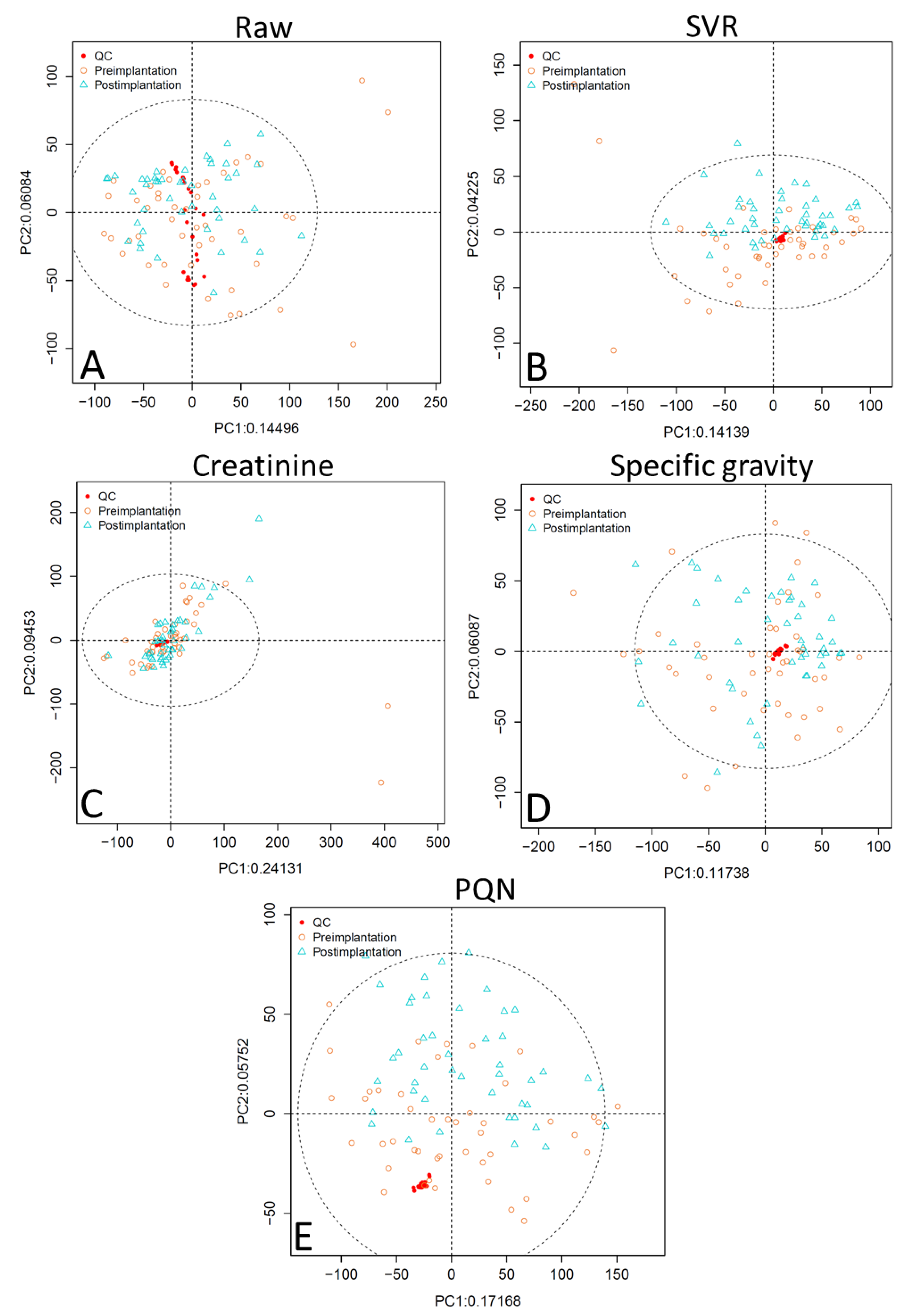
2. Results
3. Discussion
4. Materials and Methods
4.1. Study Populations
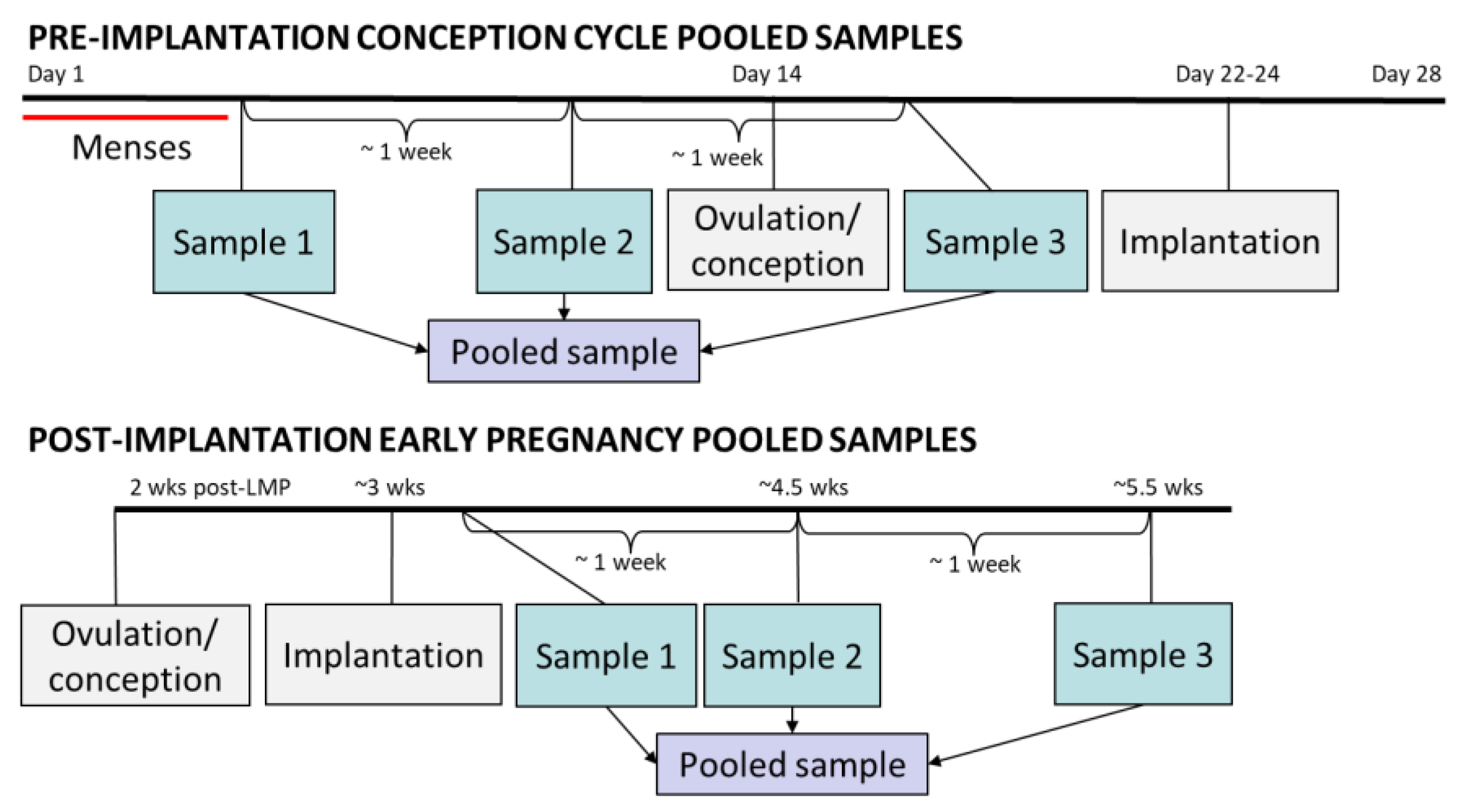
4.2. Pooled Urine Samples
4.3. Specimen Preparation
4.4. UHPLC/MS Analysis
4.5. Data Processing
4.6. Normalization Methods
4.7. Statistical Comparison of Normalization Methods
5. Conclusions
Supplementary Materials
Author Contributions
Funding
Acknowledgments
Conflicts of Interest
Appendix A. Metabolomics Data Processing Parameters
References
- Cai, Y.; Rosen Vollmar, A.K.; Johnson, C.H. Analyzing metabolomics data for environmental health and exposome research. In Computational Methods and Data Analysis for Metabolomics; Li, S., Ed.; Springer Nature: New York, NY, USA, 2019; in press. [Google Scholar]
- Robinson, O.; Vrijheid, M. The pregnancy exposome. Curr. Environ. Heal. Rep. 2015, 2, 204–213. [Google Scholar] [CrossRef] [PubMed]
- Fleming, T.P.; Watkins, A.J.; Velazquez, M.A.; Mathers, J.C.; Prentice, A.M.; Stephenson, J.; Barker, M.; Saffery, R.; Yajnik, C.S.; Eckert, J.J.; et al. Origins of lifetime health around the time of conception: Causes and consequences. Lancet 2018, 391, 1842–1852. [Google Scholar] [CrossRef]
- Barr, D.B.; Wilder, L.C.; Caudill, S.P.; Gonzalez, A.J.; Needham, L.L.; Pirkle, J.L. Urinary creatinine concentrations in the U.S. population: Implications for urinary biologic monitoring measurements. Environ. Health Perspect. 2005, 113, 192–200. [Google Scholar] [CrossRef] [PubMed]
- MacPherson, S.; Arbuckle, T.E.; Fisher, M. Adjusting urinary chemical biomarkers for hydration status during pregnancy. J. Expo. Sci. Environ. Epidemiol. 2018, 28, 481–493. [Google Scholar] [CrossRef] [PubMed]
- Miller, R.C.; Brindle, E.; Holman, D.J.; Shofer, J.; Klein, N.A.; Soules, M.R.; O’Connor, K.A. Comparison of specific gravity and creatinine for normalizing urinary reproductive hormone concentrations. Clin. Chem. 2004, 50, 924–932. [Google Scholar] [CrossRef] [PubMed]
- Carrieri, M.; Trevisan, A.; Bartolucci, G.B. Adjustment to concentration-dilution of spot urine samples: Correlation between specific gravity and creatinine. Int. Arch. Occup. Environ. Health 2001, 74, 63–67. [Google Scholar] [CrossRef]
- Hays, S.M.; Aylward, L.L.; Blount, B.C. Variation in urinary flow rates according to demographic characteristics and body mass index in NHANES: Potential confounding of associations between health outcomes and urinary biomarker concentrations. Environ. Health Perspect. 2015, 123, 293–300. [Google Scholar] [CrossRef]
- Boeniger, M.F.; Lowry, L.K.; Rosenberg, J. Interpretation of urine results used to assess chemical exposure with emphasis on creatinine adjustments: A review. Am. Ind. Hyg. Assoc. J. 1993, 54, 615–627. [Google Scholar] [CrossRef]
- Davison, J.M.; Noble, M.C. Serial changes in 24 hour creatinine clearance during normal menstrual cycles and the first trimester of pregnancy. Br. J. Obstet. Gynaecol. 1981, 88, 10–17. [Google Scholar] [CrossRef]
- Odutayo, A.; Hladunewich, M. Obstetric nephrology: Renal hemodynamic and metabolic physiology in normal pregnancy. Clin. J. Am. Soc. Nephrol. 2012, 7, 2073–2080. [Google Scholar] [CrossRef]
- Blackburn, S.T. Maternal, Fetal, and Neonatal Physiology, 3rd ed.; Elsevier: St. Louis, MO, USA, 2007. [Google Scholar]
- Abduljalil, K.; Furness, P.; Johnson, T.N.; Rostami-Hodjegan, A.; Soltani, H. Anatomical, physiological and metabolic changes with gestational age during normal pregnancy: A database for parameters required in physiologically based pharmacokinetic modelling. Clin. Pharmacokinet. 2012, 51, 365–396. [Google Scholar] [CrossRef] [PubMed]
- Cheung, K.L.; Lafayette, R.A. Renal physiology of pregnancy. Adv. Chronic Kidney Dis. 2013, 20, 209–214. [Google Scholar] [CrossRef] [PubMed]
- Weaver, V.M.; Kotchmar, D.J.; Fadrowski, J.J.; Silbergeld, E.K. Challenges for environmental epidemiology research: Are biomarker concentrations altered by kidney function or urine concentration adjustment? J. Expo. Sci. Environ. Epidemiol. 2016, 26, 1–8. [Google Scholar] [CrossRef] [PubMed]
- Aylward, L.L.; Hays, S.M.; Smolders, R.; Koch, H.M.; Cocker, J.; Jones, K.; Warren, N.; Levy, L.; Bevan, R. Sources of variability in biomarker concentrations. J. Toxicol. Environ. Heal. Part B Crit. Rev. 2014, 17, 45–61. [Google Scholar] [CrossRef] [PubMed]
- Warrack, B.M.; Hnatyshyn, S.; Ott, K.H.; Reily, M.D.; Sanders, M.; Zhang, H.; Drexler, D.M. Normalization strategies for metabonomic analysis of urine samples. J. Chromatogr. B Anal. Technol. Biomed Life Sci. 2009, 877, 547–552. [Google Scholar] [CrossRef]
- Zhang, T.; Watson, D.G. A short review of applications of liquid chromatography mass spectrometry based metabolomics techniques to the analysis of human urine. Analyst 2015, 140, 2907–2915. [Google Scholar] [CrossRef] [PubMed]
- Jacob, C.C.; Dervilly-Pinel, G.; Biancotto, G.; Le Bizec, B. Evaluation of specific gravity as normalization strategy for cattle urinary metabolome analysis. Metabolomics 2014, 10, 627–637. [Google Scholar] [CrossRef]
- Shen, X.; Gong, X.; Cai, Y.; Guo, Y.; Tu, J.; Li, H.; Zhang, T.; Wang, J.; Xue, F.; Zhu, Z.J. Normalization and integration of large-scale metabolomics data using support vector regression. Metabolomics 2016, 12, 1–12. [Google Scholar] [CrossRef]
- Kuligowski, J.; Sánchez-Illana, Á.; Sanjuán-Herráez, D.; Vento, M.; Quintás, G. Intra-batch effect correction in liquid chromatography-mass spectrometry using quality control samples and support vector regression (QC-SVRC). Analyst 2015, 140, 7810–7817. [Google Scholar] [CrossRef]
- Gagnebin, Y.; Tonoli, D.; Lescuyer, P.; Ponte, B.; de Seigneux, S.; Martin, P.Y.; Schappler, J.; Boccard, J.; Rudaz, S. Metabolomic analysis of urine samples by UHPLC-QTOF-MS: Impact of normalization strategies. Anal. Chim. Acta 2017, 955, 27–35. [Google Scholar] [CrossRef]
- Chadha, V.; Garg, U.; Alon, U.S. Measurement of urinary concentration: A critical appraisal of methodologies. Pediatr. Nephrol. 2001, 16, 374–382. [Google Scholar] [CrossRef]
- Dieterle, F.; Ross, A.; Schlotterbeck, G.; Senn, H. Probabilistic quotient normalization as robust method to account for dilution of complex biological mixtures. Application in 1H NMR metabonomics. Anal. Chem. 2006, 78, 4281–4290. [Google Scholar] [CrossRef] [PubMed]
- Di Guida, R.; Engel, J.; Allwood, J.W.; Weber, R.J.M.; Jones, M.R.; Sommer, U.; Viant, M.R.; Dunn, W.B. Non-targeted UHPLC-MS metabolomic data processing methods: A comparative investigation of normalisation, missing value imputation, transformation and scaling. Metabolomics 2016, 12, 1–14. [Google Scholar] [CrossRef] [PubMed]
- Chen, J.; Zhang, P.; Lv, M.; Guo, H.; Huang, Y.; Zhang, Z.; Xu, F. Influences of normalization method on biomarker discovery in gas chromatography-mass spectrometry-based untargeted metabolomics: What should be considered? Anal. Chem. 2017, 89, 5342–5348. [Google Scholar] [CrossRef] [PubMed]
- Filzmoser, P.; Walczak, B. What can go wrong at the data normalization step for identification of biomarkers? J. Chromatogr. A 2014, 1362, 194–205. [Google Scholar] [CrossRef]
- Edmands, W.M.B.; Ferrari, P.; Scalbert, A. Normalization to specific gravity prior to analysis improves information recovery from high resolution mass spectrometry metabolomic profiles of human urine. Anal. Chem. 2014, 86, 10925–10931. [Google Scholar] [CrossRef]
- Chetwynd, A.J.; Abdul-Sada, A.; Holt, S.G.; Hill, E.M. Use of a pre-analysis osmolality normalisation method to correct for variable urine concentrations and for improved metabolomic analyses. J. Chromatogr. A 2016, 1431, 103–110. [Google Scholar] [CrossRef]
- Gika, H.G.; Zisi, C.; Theodoridis, G.; Wilson, I.D. Protocol for quality control in metabolic profiling of biological fluids by U(H)PLC-MS. J. Chromatogr. B 2016, 1008, 15–25. [Google Scholar] [CrossRef]
- Naz, S.; Vallejo, M.; García, A.; Barbas, C. Method validation strategies involved in non-targeted metabolomics. J. Chromatogr. A 2014, 1353, 99–105. [Google Scholar] [CrossRef]
- Triba, M.N.; Le Moyec, L.; Amathieu, R.; Goossens, C.; Bouchemal, N.; Nahon, P.; Rutledge, D.N.; Savarin, P. PLS/OPLS models in metabolomics: The impact of permutation of dataset rows on the K-fold cross-validation quality parameters. Mol. Biosyst. 2015, 11, 13–19. [Google Scholar] [CrossRef]
- Ryan, D.; Robards, K.; Prenzler, P.D.; Kendall, M. Recent and potential developments in the analysis of urine: A review. Anal. Chim. Acta 2011, 684, 17–29. [Google Scholar] [CrossRef]
- Saccenti, E. Correlation patterns in experimental data are affected by normalization procedures: Consequences for data analysis and network inference. J. Proteome Res. 2017, 16, 619–634. [Google Scholar] [CrossRef]
- Khamis, M.M.; Holt, T.; Awad, H.; El-Aneed, A.; Adamko, D.J. Comparative analysis of creatinine and osmolality as urine normalization strategies in targeted metabolomics for the differential diagnosis of asthma and COPD. Metabolomics 2018, 14, 1–8. [Google Scholar] [CrossRef]
- Kennedy, A.D.; Miller, M.J.; Beebe, K.; Wulff, J.E.; Evans, A.M.; Miller, L.A.D.; Sutton, V.R.; Sun, Q.; Elsea, S.H. Metabolomic profiling of human urine as a screen for multiple inborn errors of metabolism. Genet. Test. Mol. Biomark. 2016, 20, 485–495. [Google Scholar] [CrossRef]
- Heavner, D.L.; Morgan, W.T.; Sears, S.B.; Richardson, J.D.; Byrd, G.D.; Ogden, M.W. Effect of creatinine and specific gravity normalization techniques on xenobiotic biomarkers in smokers’ spot and 24-h urines. J. Pharm. Biomed. Anal. 2006, 40, 928–942. [Google Scholar] [CrossRef]
- Haddow, J.E.; Knight, G.J.; Palomaki, G.E.; Neveux, L.M.; Chilmonczyk, B.A. Replacing creatinine measurements with specific gravity values to adjust urine cotinine concentrations. Clin. Chem. 1994, 40, 562–564. [Google Scholar]
- Sauvé, J.F.; Lévesque, M.; Huard, M.; Drolet, D.; Lavoué, J.; Tardif, R.; Truchon, G. Creatinine and specific gravity normalization in biological monitoring of occupational exposures. J. Occup. Environ. Hyg. 2015, 12, 123–129. [Google Scholar] [CrossRef]
- Wilcox, A.J.; Weinberg, C.R.; Wehmann, R.E.; Armstrong, E.G.; Canfield, R.E.; Nisula, B.C. Measuring early pregnancy loss: Laboratory and field methods. Fertil. Steril. 1985, 44, 366–374. [Google Scholar] [CrossRef]
- Wilcox, A.J.; Weinberg, C.R.; O’Connor, J.F.; Baird, D.D.; Schlatterer, J.P.; Canfield, R.E.; Armstrong, E.G.; Nisula, B.C. Incidence of early loss of pregnancy. N. Engl. J. Med. 1988, 319, 189–194. [Google Scholar] [CrossRef]
- Jukic, A.M.; Calafat, A.M.; McConnaughey, D.R.; Longnecker, M.P.; Hoppin, J.A.; Weinberg, C.R.; Wilcox, A.J.; Baird, D.D. Urinary concentrations of phthalate metabolites and bisphenol A and associations with follicular-phase length, luteal-phase length, fecundability, and early pregnancy loss. Environ. Health Perspect. 2016, 124, 321–328. [Google Scholar] [CrossRef]
- Vuckovic, D. Current trends and challenges in sample preparation for global metabolomics using liquid chromatography-mass spectrometry. Anal. Bioanal. Chem. 2012, 403, 1523–1548. [Google Scholar] [CrossRef]
- Smith, C.A.; Want, E.J.; O’Maille, G.; Abagyan, R.; Siuzdak, G. XCMS: Processing mass spectrometry data for metabolite profiling using nonlinear peak alignment, matching, and identification. Anal. Chem. 2006, 78, 779–787. [Google Scholar] [CrossRef]
- Tautenhahn, R.; Bottcher, C.; Neumann, S. Highly sensitive feature detection for high resolution LC/MS. BMC Bioinform. 2008, 9, 504. [Google Scholar] [CrossRef]
- Benton, H.P.; Want, E.J.; Ebbels, T.M.D. Correction of mass calibration gaps in liquid chromatography-mass spectrometry metabolomics data. Bioinformatics 2010, 26, 2488–2489. [Google Scholar] [CrossRef]
- Shen, X.; Zhu, Z. MetCleaning. R package version 0.99.85. 2018. [Google Scholar]
- Sánchez-Illana, Á.; Pérez-Guaita, D.; Cuesta-García, D.; Sanjuan-Herráez, J.D.; Vento, M.; Ruiz-Cerdá, J.L.; Quintás, G.; Kuligowski, J. Model selection for within-batch effect correction in UPLC-MS metabolomics using quality control—Support vector regression. Anal. Chim. Acta 2018, 1026, 62–68. [Google Scholar] [CrossRef]
- Vij, H.S.; Howell, S. Improving the specific gravity adjustment method for assessing urinary concentrations of toxic substances. Am. Ind. Hyg. Assoc. J. 1998, 59, 375–380. [Google Scholar] [CrossRef]
- Wu, Y.; Li, L. Sample normalization methods in quantitative metabolomics. J. Chromatogr. A 2016, 1430, 80–95. [Google Scholar] [CrossRef]
- Wheelock, Å.M.; Wheelock, C.E. Trials and tribulations of ’omics data analysis: Assessing quality of SIMCA-based multivariate models using examples from pulmonary medicine. Mol. Biosyst. 2013, 9, 2589–2596. [Google Scholar] [CrossRef]
- Benjamini, Y.; Hochberg, Y. Controlling the false discovery rate: A practical and powerful approach to multiple testing. J. R. Stat. Soc. Ser. B 1995, 57, 289–300. [Google Scholar] [CrossRef]


| Normalization Approach | RPLC Data | HILIC Data | ||
|---|---|---|---|---|
| Median RSD (IQR) | Peaks with RSD < 0.3, n (%) | Median RSD (IQR) | Peaks with RSD < 0.3, n (%) | |
| Raw Data | 0.23 | 9827/12,811 | 0.33 | 8271/18,977 |
| (0.16–0.29) | (76.7%) | (0.23–0.48) | (43.6%) | |
| SVR | 0.15 | 12,023/12,794 | 0.19 | 15,158/18,882 |
| (0.10–0.20) | (94.0%) | (0.13–0.27) | (80.3%) | |
| SVR and Creatinine | 0.18 | 11,744/12,794 | 0.20 | 15,104/18,882 |
| (0.15–0.23) | (91.8%) | (0.13–0.27) | (80.0%) | |
| SVR and Specific Gravity | 0.15 | 12,023/12,794 | 0.19 | 15,158/18,882 |
| (0.10–0.20) | (94.0%) | (0.13–0.27) | (80.3%) | |
| SVR and PQN | 0.08 | 12,667/12,794 | 0.11 | 18,106/18,882 |
| (0.05–0.11) | (99.0%) | (0.07–0.16) | (95.9%) | |
| Compared Normalization Approaches | RPLC Data | HILIC Data | ||
|---|---|---|---|---|
| RSD Mean Difference 3 | p-value | RSD Mean Difference 3 | p-value | |
| Raw and SVR 2 | 0.100 | p < 2.2 × 10⁻¹⁶ | 0.160 | p < 2.2 × 10⁻¹⁶ |
| SVR and Creatinine 2,4 | −0.040 | p < 2.2 × 10⁻¹⁶ | −0.002 | 0.21 |
| SVR and Specific Gravity 2,4 | 0 | -- | 0 | -- |
| SVR and PQN 2 | 0.075 | p < 2.2 × 10⁻¹⁶ | 0.100 | p < 2.2 × 10⁻¹⁶ |
| Creatinine and Specific Gravity 2,4 | 0.040 | p < 2.2 × 10⁻¹⁶ | 0.002 | 0.21 |
| Creatinine and PQN 2 | 0.116 | p < 2.2 × 10⁻¹⁶ | 0.103 | p < 2.2 × 10⁻¹⁶ |
| Specific gravity and PQN 2 | 0.075 | p < 2.2 × 10⁻¹⁶ | 0.101 | p < 2.2 × 10⁻¹⁶ |
| Normalization Approach | RPLC Data | HILIC Data | ||||||||
|---|---|---|---|---|---|---|---|---|---|---|
| Features, n 3 | R2X | R2Y | Q2 | VIP > 1 and q < 0.05, n 4 | Features, n 3 | R2X | R2Y | Q2 | VIP > 1 and q < 0.05, n 4 | |
| Raw 2 | 9816 | 0.18 | 0.93 | 0.66 | 1303 | 8271 | 0.25 | 0.87 | 0.51 | 1385 |
| SVR 2 | 12,023 | 0.13 | 0.95 | 0.62 | 1425 | 15,158 | 0.22 | 0.90 | 0.49 | 2161 |
| Creatinine 2 | 11,744 | 0.36 | 0.82 | 0.58 | 1589 | 15,104 | 0.37 | 0.75 | 0.27 | 1491 |
| Specific Gravity 2 | 12,023 | 0.37 | 0.86 | 0.62 | 1591 | 15,158 | 0.20 | 0.87 | 0.53 | 2358 |
| PQN2 | 12,667 | 0.18 | 0.94 | 0.69 | 1551 | 18,106 | 0.25 | 0.91 | 0.52 | 2578 |
© 2019 by the authors. Licensee MDPI, Basel, Switzerland. This article is an open access article distributed under the terms and conditions of the Creative Commons Attribution (CC BY) license (http://creativecommons.org/licenses/by/4.0/).
Share and Cite
Rosen Vollmar, A.K.; Rattray, N.J.W.; Cai, Y.; Santos-Neto, Á.J.; Deziel, N.C.; Jukic, A.M.Z.; Johnson, C.H. Normalizing Untargeted Periconceptional Urinary Metabolomics Data: A Comparison of Approaches. Metabolites 2019, 9, 198. https://doi.org/10.3390/metabo9100198
Rosen Vollmar AK, Rattray NJW, Cai Y, Santos-Neto ÁJ, Deziel NC, Jukic AMZ, Johnson CH. Normalizing Untargeted Periconceptional Urinary Metabolomics Data: A Comparison of Approaches. Metabolites. 2019; 9(10):198. https://doi.org/10.3390/metabo9100198
Chicago/Turabian StyleRosen Vollmar, Ana K., Nicholas J. W. Rattray, Yuping Cai, Álvaro J. Santos-Neto, Nicole C. Deziel, Anne Marie Z. Jukic, and Caroline H. Johnson. 2019. "Normalizing Untargeted Periconceptional Urinary Metabolomics Data: A Comparison of Approaches" Metabolites 9, no. 10: 198. https://doi.org/10.3390/metabo9100198
APA StyleRosen Vollmar, A. K., Rattray, N. J. W., Cai, Y., Santos-Neto, Á. J., Deziel, N. C., Jukic, A. M. Z., & Johnson, C. H. (2019). Normalizing Untargeted Periconceptional Urinary Metabolomics Data: A Comparison of Approaches. Metabolites, 9(10), 198. https://doi.org/10.3390/metabo9100198