A Noniterative Radix-8 CORDIC Algorithm with Low Latency and High Efficiency

Abstract

An efficient, noniterative Radix-8 (NR-8) coordinate rotation digital computer (CORDIC) algorithm is proposed for low-latency and high-efficiency computation of the functions of sine, cosine, or the phase shift, with which the values of the functions are precisely computed by only using the angle in a narrow range of [0, π/12] rather than in a wide angle range of [0, π/2]. This algorithm is expressed by a formula that simplifies the traditional iterative processes by using a complex multiplier. The results obtained from the simulation and the experiment on an FPGA show that the NR-8 CORDIC algorithm operates well, with which the 16-bit precision output is extremely precise, with only 0.012% of the absolute error for computing the sine or cosine function with a step of 0.001°. Compared with the best conventional CORDIC algorithm, the clock latency of this algorithm significantly decreases down to less than 50%, only needs half of the logic resources and consumes half of the power. This algorithm also takes advantages over other newly improved CORDIC algorithms and requires less than half of the clock latency, even for a 23-bit precision output. Therefore, this algorithm could provide a potential application in real-time systems such as radar digital beamforming.

1. Introduction

As one of the most common transcendental functions, the sine or cosine function has been widely used in real-time digital signal processing systems, such as radar, ultrasound, robotics, communication and so on [1,2,3,4,5,6,7]. The accuracy and efficiency of the computation of the functions are two key requirements for evaluating the performance of these systems. For this purpose, many methods to calculating the sine or cosine function have been developed, such as the lookup table, Taylor series, polynomial approximation and so on [8,9,10]. However, these methods have the disadvantage of either high complexity or high latency, and thus an efficient method is extremely required to meet the accurate and efficient computation for real-time systems. Fortunately, the coordinate rotation digital computer (CORDIC) algorithm [11] can provide accurate and efficient computations by employing an iterative way and decomposing the calculation into a series of addition, subtraction and shift operations, which enables it to be widely used in digital circuits to implement the computations of trigonometric and exponential functions, and so forth [12]. However, as an iterative algorithm, the accuracy of the CORDIC algorithm strongly relies on the number of iterations, so the increase of the iteration number leads to the increase of the clock latency, thus lowering the efficiency for the computations.

To further enhance the efficiency, more progress has been made by improving the architecture of the CORDIC algorithm to achieve a more efficient algorithm, such as the Scaling-Free (SF) CORDIC, Radix-4 CORDIC, Radix-8 CORDIC and low-latency Hybrid (LLH) CORDIC algorithms [13,14,15,16,17]. Some of the improved CORDIC algorithms have been widely used in radar digital beamforming (DBF) systems. For instance, Lee et al. developed a CORDIC-based algorithm to be used in Multi-Gbps MIMO systems, which is implemented by a Virtex-6 FPGA using 49,752 slices, and the algorithm needs 260 ns (250 MHz, 65 clock periods) of latency due to the many iterations required for computations [4]. Similarly, Jun et al. described look-ahead, pipelined CORDIC-based adaptive filters and their application to adaptive beamforming [5], and the pipeline level m depends on the m-bit precision. However, the CORDIC algorithm often requires many iterations to converge, which has become a major bottleneck for real-time applications.

In this work, a new noniterative Radix-8 (NR-8) CORDIC algorithm is proposed for low-latency implementation on FPGAs. In the process of the development of an NR-8 CORDIC algorithm, three steps were taken: (1) The NR-8 CORDIC algorithm was derived from the conventional Radix-2 CORDIC one. (2) The input angle θ was set to a narrow range by simultaneously transforming the input variables $x_0$ and $y_0$. (3) A formula was deduced and optimized. These steps can narrow the selected range of the iteration angle and realize a noniterative formula of the CORDIC algorithm; besides, the algorithm can be accelerated by the multiplier module readily available in FPGAs [18]. As a result, the algorithm can reduce 7–17 clock latencies of the conventional CORDIC (16-bit precision) algorithm to a three-clock latency, needs less logic resources and consumes less power. Compared with the LLH algorithm [16], it has great advantages in terms of time and resources. For the structure of this paper, following the introduction is Section 2, in which the derivation from the conventional CORDIC algorithm is presented. In Section 3, the proposed NR-8 CORDIC is introduced. Section 4 presents its FPGA implementation and analysis. Section 5 introduces the application of the NR-8 CORDIC in radar DBF. Finally, a conclusion is made according to the results obtained from the above sections.

2. Conventional CORDIC Rotator Algorithm

The CORDIC algorithm usually operates in rotation mode or vector mode [11,12], following linear, circular or hyperbolic coordinate trajectories. In this paper, we focus on the rotation mode using circular trajectory.

The rotation mode is depicted in Figure 1, where $\theta$ is the angle between the ${\stackrel{\rightharpoonup }{V}}_0(x_0,y_0)$ and ${\stackrel{\rightharpoonup }{V}}_d(x_d,y_d)$ vectors. As the vector ${\stackrel{\rightharpoonup }{V}}_0$ rotates counterclockwise to the vector ${\stackrel{\rightharpoonup }{V}}_d$, the coordinate, $(x_d,y_d)$, can be described as in Equation (1):

$$\left[\begin{array}{l}{x}_d\\ y_d\end{array}\right]=\left[\begin{array}{cc}\cos \theta & -\sin \theta \\ \sin \theta & \cos \theta \end{array}\right] \left[\begin{array}{l}{x}_0\\ y_0\end{array}\right]=\cos \theta \left[\begin{array}{cc}1& -\tan \theta \\ \tan \theta & 1\end{array}\right]\left[\begin{array}{l}{x}_0\\ y_0\end{array}\right]$$

(1)

If the initial vector $(x_0,y_0)$ is set to $x_0=1,y_0=0$, Equation (1) can be used to compute $\cos \theta$ and $\sin \theta$.

$\theta$ is decomposed into a series of micro angles, each of which corresponds to one step rotation as shown in Figure 1 and described as in Equation (2):

$$\theta ={\displaystyle \sum _{i=0}^n{\theta }_i},{\theta }_i={\tan }^{-1}({\sigma }_i{\mathrm{R}}^{-(i+1)})$$

(2)

where n denotes the number of rotations, R denotes the radix, $\mathrm{R}=2^l,l\in \mathbf{N}$, ${\theta }_i$ denotes micro angles and ${\sigma }_i$ is the selection factors defined as all integers within the interval ${\sigma }_i\in [-\mathrm{R}/2,\mathrm{R}/2]$.

Substituting Equation (2) into Equation (1) yields Equation (3):

$$\left[\begin{array}{l}{x}_d\\ y_d\end{array}\right]={\displaystyle \prod _{i=0}^n\left[\begin{array}{cc}\cos {\theta }_i& -\sin {\theta }_i\\ \sin {\theta }_i& \cos {\theta }_i\end{array}\right]\left[\begin{array}{l}{x}_0\\ y_0\end{array}\right]}=\left[{\displaystyle \prod _{i=0}^n\cos {\theta }_i}\right]\times {\displaystyle \prod _{i=0}^n\left[\begin{array}{cc}1& -\tan {\theta }_i\\ \tan {\theta }_i& 1\end{array}\right]}\left[\begin{array}{l}{x}_0\\ y_0\end{array}\right]$$

(3)

Equation (3) describes the computation process illustrated in Figure 1.

Apparently, the recursion formula of the ith rotation can be written as Equation (4):

$$\left[\begin{array}{l}{x}_{i+1}\\ y_{i+1}\end{array}\right]=\cos {\theta }_i\left[\begin{array}{cc}1& -\tan {\theta }_i\\ \tan {\theta }_i& 1\end{array}\right]\left[\begin{array}{l}{x}_i\\ y_i\end{array}\right]$$

(4)

If R equals 2, it is the conventional Radix-2 (R-2) CORDIC iterative algorithm. If R equals 4, it becomes a conventional Radix-4 (R-4) CORDIC iterative algorithm. If R equals 8, it becomes a conventional Radix-8 (R-8) CORDIC iterative algorithm, and thus Equation (3) can be written as Equation (5):

$$\left[\begin{array}{l}{x}_d\\ y_d\end{array}\right]=K\times {\displaystyle \prod _{i=0}^n\left[\begin{array}{cc}1& -{\sigma }_i{\mathrm{R}}^{-\left(i+1\right)}\\ {\sigma }_i{\mathrm{R}}^{-\left(i+1\right)}& 1\end{array}\right]}\left[\begin{array}{l}{x}_0\\ y_0\end{array}\right]$$

(5)

where the scale factor K is defined as Equation (6):

$$K={\displaystyle \prod _{i=0}^n\cos {\theta }_i=}{\displaystyle \prod _{i=0}^n{\left(1+{\sigma }_i^2{\mathrm{R}}^{-2\left(i+1\right)}\right)}^{1/2}}$$

(6)

The conventional CORDIC algorithm is implemented in an iterative fashion, in which the input angle is completed by a step-by-step mode using the series of micro angles. After the ith iteration, the residual error angle is defined as in Equation (7):

$$z_{i+1}=\theta -{\displaystyle \sum _{j=0}^i{\theta }_j},i=0,1,2,\cdots n$$

(7)

where $z_0=\theta$. For the next iteration, an optimal factor ${\sigma }_{i+1}$ is selected so that the residual error angle becomes minimal, which can be calculated by using Equation (8):

$${\sigma }_i=\mathrm{argmin}\left|z_i-{\sigma }_i{\mathrm{R}}^{-(i+1)}\right|=\mathrm{argmin}\left|{\omega }_i-{\sigma }_i\right|,s.t. {\sigma }_i\in [-\mathrm{R}/2,\mathrm{R}/2]$$

(8)

where ${\omega }_i=z_i{\mathrm{R}}^{i+1}$. It can be directly solved using a rounding operation via Equation (9):

$${\sigma }_i=\{\begin{array}{ll}\mathrm{R}/2,& {\omega }_i\ge (\mathrm{R}-1)/2\\ -\mathrm{R}/2,& {\omega }_i\le -(\mathrm{R}-1)/2\\ U({\omega }_i),& \mathrm{else}\end{array}$$

(9)

where the function $U({\omega }_i)$ rounds each element of ${\omega }_i$ to the nearest integer.

In each iteration, as the R number increases, the number of iterations decreases, but the selection factor ${\sigma }_i$ increases, thus increasing the complexity of the conventional CORDIC algorithm. Hence, we found that R-8 CORDIC (R = 8) is a good balance between complexity and efficiency. However, the current iterative R-8 algorithm still needs several iterations. For example, six iterations are necessary for a 16-bit depth digital signal processing application. To address this problem, this paper proposes a noniterative form of the R-8 CORDIC (NR-8 CORDIC) algorithm.

3. Noniterative Radix-8 CORDIC Algorithm

We propose a noniterative computation structure of the R-8 CORDIC algorithm by iterating the data in a narrow input angle interval, using an explicit formula of solution, simplifying the scale factor and transforming the input variables $x_0$ and $y_0$ to accelerate the convergence of the algorithm.

3.1. Narrow Input Angle θ Range

Conventionally, one only needs to consider the input angle $\theta \in [0,\pi /2]$ of the first quadrant, from which the rest of the quadrants can be easily computed by invoking the symmetry property of the sine or cosine function. Thus, the rest of the quadrants can be mapped to the first quadrant by simple transformation. In this article, we first narrow the input angle interval into an angle range of $[0,\pi /12]$.

The first quadrant of the coordinate system is equally divided into six regions, marked from A to F, the range of which becomes $[0,\pi /12]$. Then the angle $\theta \in [0,\pi /2]$ can be folded to the range of $\phi \in [0,\pi /12]$. The CORDIC output mappings between $\theta$ and $\phi$ are given in

Table 1. The CORDIC output mappings between θ and φ.

Regions	$\mathit{\theta }$	${\mathit{x}}_0^{\prime },{\mathit{y}}_0^{\prime }$	${\mathit{x}}_{\mathit{d}},{\mathit{y}}_{\mathit{d}}$
$A, [0,\frac{\pi }{12})$	$\phi$	$\left[\begin{array}{l}{x}_0^{\prime }\\ y_0^{\prime }\end{array}\right]=\left[\begin{array}{l}{x}_0\\ y_0\end{array}\right]$	$\left[\begin{array}{l}{x}_d\\ y_d\end{array}\right]=\mathit{R}\mathit{T}(\theta )\left[\begin{array}{l}{x}_0^{\prime }\\ y_0^{\prime }\end{array}\right]$
$B, [\frac{\pi }{12},\frac{\pi }{6})$	$\frac{\pi }{6}-\phi$	$\left[\begin{array}{l}{x}_0^{\prime }\\ y_0^{\prime }\end{array}\right]=\frac{1}{2}\left[\begin{array}{l}\sqrt{3}{x}_0-y_0\\ -x_0-\sqrt{3}{y}_0\end{array}\right]$	$\left[\begin{array}{l}{x}_d\\ -y_d\end{array}\right]=\mathit{R}\mathit{T}(\theta )\left[\begin{array}{l}{x}_0^{\prime }\\ y_0^{\prime }\end{array}\right]$
$C, [\frac{\pi }{6},\frac{\pi }{4})$	$\frac{\pi }{6}+\phi$	$\left[\begin{array}{l}{x}_0^{\prime }\\ y_0^{\prime }\end{array}\right]=\frac{1}{2}\left[\begin{array}{l}\sqrt{3}{x}_0-y_0\\ x_0-\sqrt{3}{y}_0\end{array}\right]$	$\left[\begin{array}{l}{x}_d\\ y_d\end{array}\right]=\mathit{R}\mathit{T}(\theta )\left[\begin{array}{l}{x}_0^{\prime }\\ y_0^{\prime }\end{array}\right]$
$D, [\frac{\pi }{4},\frac{\pi }{3})$	$\frac{\pi }{3}-\phi$	$\left[\begin{array}{l}{x}_0^{\prime }\\ y_0^{\prime }\end{array}\right]=\frac{1}{2}\left[\begin{array}{l}{x}_0-\sqrt{3}{y}_0\\ \sqrt{3}{x}_0-y_0\end{array}\right]$	$\left[\begin{array}{l}{x}_d\\ -y_d\end{array}\right]=\mathit{R}\mathit{T}(\theta )\left[\begin{array}{l}{x}_0^{\prime }\\ y_0^{\prime }\end{array}\right]$
$E, [\frac{\pi }{3},\frac{5\pi }{12})$	$\frac{\pi }{3}+\phi$	$\left[\begin{array}{l}{x}_0^{\prime }\\ y_0^{\prime }\end{array}\right]=\frac{1}{2}\left[\begin{array}{l}{x}_0-\sqrt{3}{y}_0\\ \sqrt{3}{x}_0+y_0\end{array}\right]$	$\left[\begin{array}{l}{x}_d\\ y_d\end{array}\right]=\mathit{R}\mathit{T}(\theta )\left[\begin{array}{l}{x}_0^{\prime }\\ t_0^{\prime }\end{array}\right]$
$F, [\frac{5\pi }{12},\frac{\pi }{2}]$	$\frac{\pi }{2}-\phi$	$\left[\begin{array}{l}{x}_0^{\prime }\\ y_0^{\prime }\end{array}\right]=\left[\begin{array}{l}-x_0\\ -y_0\end{array}\right]$	$\left[\begin{array}{l}{x}_d\\ -y_d\end{array}\right]=\mathit{R}\mathit{T}(\theta )\left[\begin{array}{l}{x}_0^{\prime }\\ y_0^{\prime }\end{array}\right]$

. Accordingly, the input variables $x_0,y_0$ need to be changed to $x_0^{\prime },y_0^{\prime }$, respectively. Therefore, we can readily compute the output values in the angle range of $\phi$ according to the CORDIC algorithm, on the base of which, and as shown in Table 1, the output values $x_d,y_d$ in the whole range of $\theta$ are achieved with ease ($\sqrt{3}$ is calculated by using the Taylor series, and a matrix is defined as $\mathit{R}\mathit{T}(\theta )=\left[\begin{array}{cc}\cos \theta & -\sin \theta \\ \sin \theta & \cos \theta \end{array}\right]$).

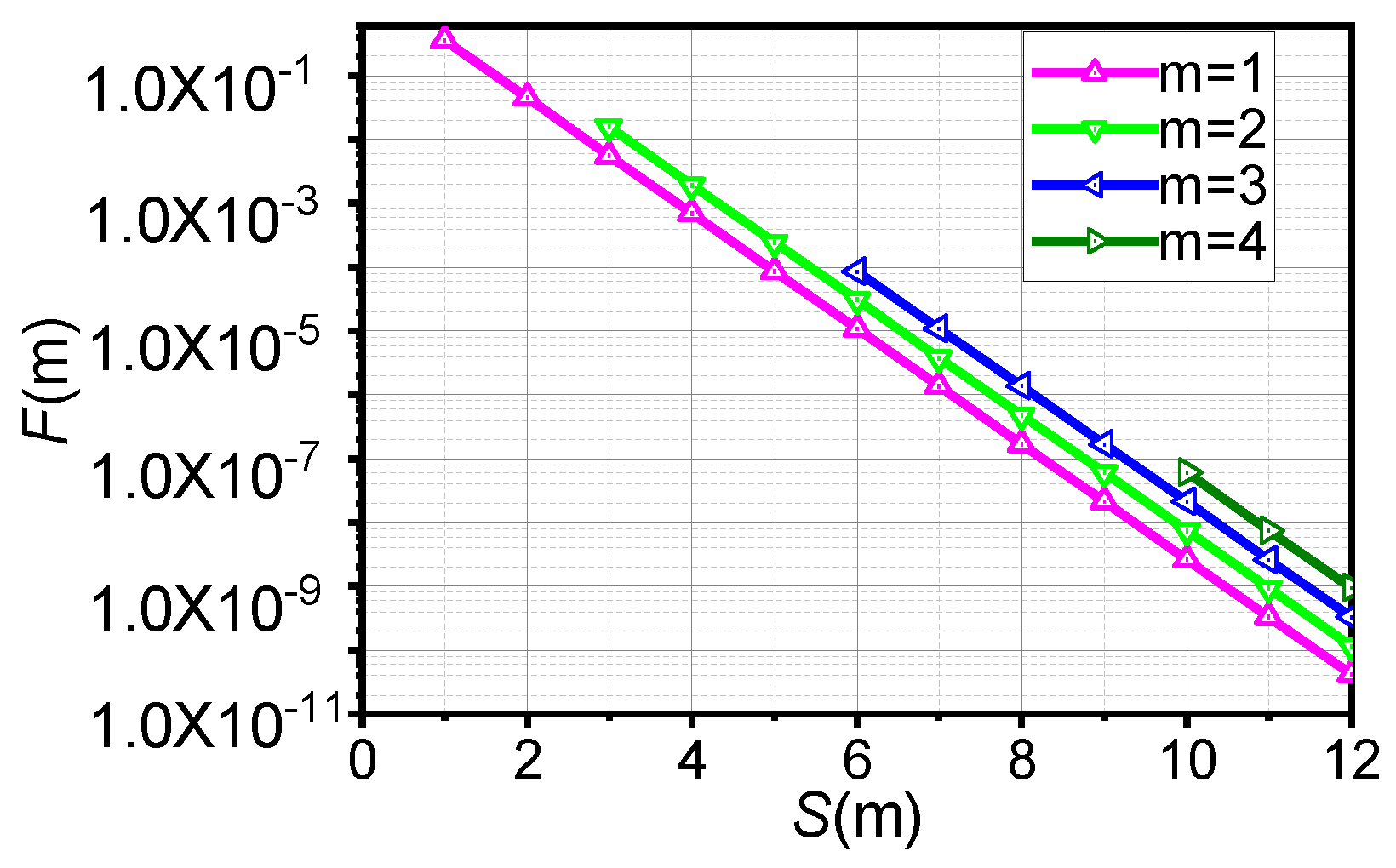
3.2. Explicit Formula of Convergence

Equation (5) can be computed naturally by using iterations. The scale factor K is temporarily ignored for the sake of simplicity. The iterative formula of Equation (5) is given as follows. Let us define

$$a_i={\sigma }_i{8}^{-(i+1)}$$

(10)

If i = 1, then

$$\{\begin{array}{l}{x}_1=x_0-a_0{y}_0\\ y_1=y_0+a_0{x}_0\end{array}.$$

If i = 2, then

$$\{\begin{array}{l}{x}_2=\left(1-a_0{a}_1\right)x_0-\left(a_0+a_1\right)y_0\\ y_2=\left(1-a_0{a}_1\right)y_0+\left(a_0+a_1\right)x_0\end{array}.$$

If i = 3, then

$$\{\begin{array}{l}{x}_3=\left(1-a_0{a}_1-a_0{a}_2-a_1{a}_2\right)x_0-\left(a_0+a_1+a_2-a_0{a}_1{a}_2\right)y_0\\ y_3=\left(1-a_0{a}_1-a_0{a}_2-a_1{a}_2\right)y_0+\left(a_0+a_1+a_2-a_0{a}_1{a}_2\right)x_0\end{array}.$$

If i = 4, then

$$\{\begin{array}{l}{x}_4=\left(1-a_0{a}_1-a_0{a}_2-a_0{a}_3-a_1{a}_2-a_1{a}_3-a_2{a}_3+a_0{a}_1{a}_2{a}_3\right)x_0-\left(a_0+a_1+a_2+a_3-a_0{a}_1{a}_2-a_0{a}_1{a}_3-a_0{a}_2{a}_3-a_1{a}_2{a}_3\right)y_0\\ y_4=\left(1-a_0{a}_1-a_0{a}_2-a_0{a}_3-a_1{a}_2-a_1{a}_3-a_2{a}_3+a_0{a}_1{a}_2{a}_3\right)y_0+\left(a_0+a_1+a_2+a_3-a_0{a}_1{a}_2-a_0{a}_1{a}_3-a_0{a}_2{a}_3-a_1{a}_2{a}_3\right)x_0\end{array}$$

(11)

A deductive formula can be summarized as

$$\{\begin{array}{l}{x}_n=A_n\times x_0-B_n\times y_0\\ y_n=A_n\times y_0 +B_n\times x_0\end{array}$$

(12)

where $A_n,B_n$ are respectively defined as

$$\{\begin{array}{l}{A}_n=1-{\displaystyle {\displaystyle \sum }_{i=1}^k}{\left(-1\right)}^{i+1}{f}_a\left(C_n^{2i}\right),\hspace{1em}\hspace{1em}\hspace{1em}\hspace{1em}n\in \mathbf{N}\\ B_n=\{\begin{array}{cc}{\displaystyle {\displaystyle \sum }_{i=1}^k}{\left(-1\right)}^{i+1}{f}_a\left(C_n^{2i-1}\right),& n=2k,k\in \mathbf{N}\\ {\displaystyle {\displaystyle \sum }_{i=0}^k}{\left(-1\right)}^i{f}_a\left(C_n^{2i+1}\right),& n=2k+1,k\in \mathbf{N}\end{array}\end{array}$$

(13)

where the function of $f_a(C_n^m)$, $0\le m\le n$ is defined as the product of m different elements selected from the sets $\left\{a_0,a_1,\cdots a_{n-1}\right\}$, as described in Equation (14):

$$f_a\left(C_n^m\right)=a_{i_1}{a}_{i_2}\dots a_{i_m}, (i_1,i_1,\dots i_m)\in \left\{I\left(m\right)\right\}$$

(14)

where $\left\{I\left(m\right)\right\}$ denotes all possible combinatorial sets of m unique indices selected from $\left\{0,1,\cdots n-1\right\}$. Apparently, there are a total of $C_n^m$ sets in $\left\{I\left(m\right)\right\}$. Substituting Equation (10) into the products in Equation (14), we have the following inequality:

$$F\left(m\right)=\left|a_{i_1}{a}_{i_2}\dots a_{i_m}\right|=\left|\frac{{\sigma }_{i_1}{\sigma }_{i_2}\dots {\sigma }_{i_m}}{8^{S\left(m\right)}}\right|\le \frac{4^m}{8^{S\left(m\right)}}$$

(15)

where

$$S\left(m\right)=\left(i_1+1\right)+\left(i_2+1\right)+\dots +\left(i_m+1\right)$$

(16)

Note that the equality in Equation (15) holds if and only if $\left|{\sigma }_{i_1}\right|=\left|{\sigma }_{i_2}\right|=\dots =\left|{\sigma }_{i_m}\right|=4$. It can be observed that Equation (16) has a minimum of $S\left(m\right)=\frac{\left(1+m\right)m}{2}$.

Figure 2 shows that F(m) quickly vanishes as m or S(m) increases, from which we have two observations as follows:

• Observation (1): If $m\ge 3$, when $S\left(m\right)\ge 7$, $F\left(m\right)<0.000031$, which can be ignored.
• Observation (2): If $m=1$ or $m=2$, when $S\left(m\right)\ge 6$, $F\left(m\right)<0.000061$, which can be ignored.

Note that $S\left(m\right)\ge 8$ is necessary in order to achieve a high accuracy. Thus, we can ignore the terms that satisfy any of the above two conditions in $f_a\left(C_n^m\right)$ of Equation (13) to greatly simplify computation. For example, the terms of $a_0{a}_1{a}_2,$ $a_0{a}_2{a}_3,$ $\cdots , a_1{a}_2{a}_3,$ $\cdots ,$ $a_0{a}_1{a}_2{a}_3,$ $\cdots , a_1{a}_2{a}_3{a}_4,$ $a_0{a}_1{a}_2$…$a_2{a}_3{a}_4,$ and $a_0{a}_3,a_0{a}_4,\cdots ,a_1{a}_2,\cdots ,a_2{a}_3,\cdots ,a_4,a_5,$… can be ignored. Thus, the variables of $A_n,B_n$ in Equation (13) can be simplified as

$$\left[\begin{array}{c}{A}_n\\ B_n\end{array}\right]=\left[\begin{array}{c}1-a_0{\displaystyle {\displaystyle \sum }_{i=1}^3}{a}_i-a_1{a}_2\\ {\displaystyle {\displaystyle \sum }_{i=0}^4}{a}_i\end{array}\right] \mathrm{or}\left[\begin{array}{c}1-a_0{\displaystyle {\displaystyle \sum }_{i=1}^n}{a}_i-a_1{\displaystyle {\displaystyle \sum }_{i=2}^n}{a}_i\\ {\displaystyle {\displaystyle \sum }_{i=0}^4}{a}_i\end{array}\right]$$

(17)

3.3. Scale Factor

Now we consider the scale factor K of Equation (6). It can be written as a Taylor series, i.e.,

$$K={\displaystyle \prod }_{i=0}^n\left(1-\frac{1}{2}{a}_i^2+\frac{3}{8}{a}_i^4-\frac{5}{16}{a}_i^6+\dots \right)\approx C-\frac{1}{2}{a}_1^2$$

(18)

where $C=1-\frac{1}{2}{a}_0^2+\frac{3}{8}{a}_0^4$, and apparently we can calculate all the values of C and $\frac{1}{2}{a}_1^2$ by enumerating all values of $a_0$ and $a_1^2$, respectively. In order to speed up the parallel computation of the NR-8 CORDIC algorithm, we can compensate the input variables $x_0,y_0$ instead of $A_n,B_n$ by the scale factor K. More details about this process are described in the oncoming section.

3.4. Transformation of the Inputs $x_0$ and $y_0$

According to Table 1, the input angle $\theta \in [0,\pi /2]$ can be folded to the range of $[0,\pi /12]$. Accordingly, the input variable $x_0,y_0$ should also be transformed to $x_0^{\prime },y_0^{\prime }$. The transformation rules are as follows:

• If $\theta \in [0,\pi /12)$, then $\left[\begin{array}{l}{x}_0^{\prime }\\ y_0^{\prime }\end{array}\right]=\left[\begin{array}{l}{x}_0\\ y_0\end{array}\right]$.
• If $\theta \in [\frac{\pi }{12},\frac{\pi }{6})$, then $\left[\begin{array}{l}{x}_0^{\prime }\\ y_0^{\prime }\end{array}\right]=\frac{1}{2}\left[\begin{array}{l}\sqrt{3}{x}_0-y_0\\ -x_0-\sqrt{3}{y}_0\end{array}\right]$.
• If $\theta \in [\frac{\pi }{6},\frac{\pi }{4})$, then $\left[\begin{array}{l}{x}_0^{\prime }\\ y_0^{\prime }\end{array}\right]=\frac{1}{2}\left[\begin{array}{l}\sqrt{3}{x}_0-y_0\\ x_0-\sqrt{3}{y}_0\end{array}\right]$.
• If $\theta \in [\frac{\pi }{4},\frac{\pi }{3})$, then $\left[\begin{array}{l}{x}_0^{\prime }\\ y_0^{\prime }\end{array}\right]=\frac{1}{2}\left[\begin{array}{l}{x}_0-\sqrt{3}{y}_0\\ \sqrt{3}{x}_0-y_0\end{array}\right]$.
• If $\theta \in [\frac{\pi }{3},\frac{5\pi }{12})$, then $\left[\begin{array}{l}{x}_0^{\prime }\\ y_0^{\prime }\end{array}\right]=\frac{1}{2}\left[\begin{array}{l}{x}_0-\sqrt{3}{y}_0\\ \sqrt{3}{x}_0+y_0\end{array}\right]$.
• If $\theta \in [\frac{5\pi }{12},\frac{\pi }{2}]$, then $\left[\begin{array}{l}{x}_0^{\prime }\\ y_0^{\prime }\end{array}\right]=\left[\begin{array}{l}-x_0\\ -y_0\end{array}\right]$.

$\sqrt{3}$ can be calculated by using the Taylor series, which is $\sqrt{3}=2-\frac{1}{4}-\frac{1}{64}-\frac{1}{512}=1.732$. The input variable $x_0^{\prime },y_0^{\prime }$ is multiplied by the scale factor K to compensate loss gain due to iteration, which produces two new variables, $x_0^{″},y_0^{″}$, described as,

$$\left[\begin{array}{c}{x}_0^{″}\\ y_0^{″}\end{array}\right]=K\times \left[\begin{array}{c}{x}_0^{\prime }\\ y_0^{\prime }\end{array}\right]$$

(19)

Let $A=A_n,B=B_n$ and the explicit formula of $x_n$ and $y_n$ in Equation (12) can be rewritten as

$$\{\begin{array}{c}{x}_n=A\times x_0^{″}-B\times y_0^{″}\\ y_n=A\times y_0^{″}+B\times x_0^{″}\end{array}\iff \left(x_n+y_{n}i\right)=\left(A+Bi\right)\times \left(x_0^{″}+y_0^{″}i\right)$$

(20)

As a result, the final outputs $x_d,y_d$ in Equation (1) can be expressed by $x_n,y_n$ in Equation (20), respectively, and Equation (20) can be easily implemented by using complex multiplication [19].

4. Implementation and Analysis

In this section, the architecture and performance of the NR-8 CORDIC algorithm are discussed with a simulation and an FPGA implementation.

4.1. Noniterative Implementation

After narrowing the input angle range from $\theta$ to $\phi$, we set the initial angle of ${\mathrm{z}}_0$ in Equation (7) to be ${\mathrm{z}}_0=\phi \in \left[0,\pi /12\right]$. Thus, we have $w_0=z_0\mathrm{R}=8\phi$ and $8\phi \in \left[0,2\pi /3\right]$, so $8\phi <2.5$. Following from Equations (7)–(9), ${\sigma }_0$ is obtained as ${\sigma }_0=U\left(w_0\right)$ = $U\left(8\phi \right)$, ($U\left(8\phi \right)$ rounds each element of $8\phi$ to the nearest integer and $U\left(8\phi \right)\in \left\{0,1,2\right\}$). Subsequently, the residual $z_1$ can be described as,

$$z_1=z_0-{\tan }^{-1}({\sigma }_0/8)=\{\begin{array}{cc}{z}_0& {\sigma }_0=0\\ z_0-{\tan }^{-1}\left(1/8\right)& {\sigma }_0=1\\ z_0-{\tan }^{-1}\left(1/4\right)& {\sigma }_0=2\end{array}$$

(21)

Apparently, ${\tan }^{-1}(•)$ in Equation (21) has only three values, which can be implemented by using a small look-up table or registers.

For the residual $z_i,i\ge 2$, $z_i$ can be described as,

$$z_i=z_{i-1}-{\tan }^{-1}{\sigma }_{i-1}{8}^{-i}\approx z_{i-1}-{\sigma }_{i-1}{8}^{-i}$$

(22)

where an approximation of ${\tan }^{-1}(x)\approx x,x<1/16$ is taken. The error bound of such an approximation can be easily estimated to be 8.119 × 10⁻⁵.

By considering m-bit fixed-point processing, where all variables are stored in an FPGA as m-bit integers, we use $Z_i,i=0,1,2,\dots$ to denote the fixed-point integer of $z_i,i=0,1,2,\dots$ (i.e., $Z_i=\lfloor z_i{2}^m\rfloor$) for the sake of simplicity, where $\lfloor •\rfloor$ denotes rounding down.

From Equation (21), it can be found that the residual error angle is $\left|z_1\right|<1/8$ (i.e., $\left|Z_1\right|=\left|z_1{2}^m\right|<2^{m-3}$) so the bit width of $Z_1$ is m−2. To denote the bit width of an n-bit fixed-point variable X, we use the form of $\mathrm{X}\left[n-1 : 0\right]$. For example, $Z_1$ is expressed as $Z_1\left[m-3 : 0\right]$.

Now, let us expand $Z_1$ to the following form,

$$Z_1=Z_1\left[m-3:m-7\right]2^{m-7}+Z_1\left[m-8:m-10\right]2^{m-10}+\dots +Z_1\left[m-2-3\times q:0\right]$$

(23)

where $q=\lceil \frac{m-5}{3}\rceil$. Here, $\lceil •\rceil$ denotes rounding up.

Accordingly, $z_1$ can be rewritten as,

$$\begin{array}{ll}{z}_1& =Z_1\left[m-3:m-7\right]2^{-7}+Z_1\left[m-8:m-10\right]2^{-10}+\dots +Z_1\left[m-2-3\times q:0\right]2^{-m}\\ & ={\tan }^{-1}\left(Z_1\left[m-3:m-7\right]2^{-7}\right)+{\tan }^{-1}\left(Z_1\left[m-8:m-10\right]2^{-10}\right)+\dots +{\tan }^{-1}\left(Z_1\left[m-2-3\times q:0\right]2^{-m}\right)\end{array}$$

(24)

According to Equation (2), ${\theta }_i={\tan }^{-1}\left({\sigma }_i{8}^{-\left(i+1\right)}\right)$, we found that the variables ${\sigma }_1$, ${\sigma }_2$, … ${\sigma }_q$ and $a_1$, $a_2$, … $a_q$ (in Equation (10), $a_i={\sigma }_i{8}^{-(i+1)}$) should be selected, which can satisfy both the computation of Equation (5) and automatically fulfill the equation of $\theta ={\displaystyle {\displaystyle \sum }_{i=0}^q}{\theta }_i$. Thus, it is not necessary to follow the iterative formula of the solutions in Equations (8) and (9). Instead, from the proposed expansion in Equations (23) and (24), we can directly give the variables as,

$$\{\begin{array}{c}{\sigma }_1=Z_1\left[m-3:m-7\right]\\ {\sigma }_2=Z_1\left[m-8:m-10\right]\\ ⋮\\ {\sigma }_q=Z_1\left[m-2-3\times q:0\right]\end{array}$$

(25)

$$a_i=\{\begin{array}{cc}{\sigma }_0{2}^{-3},& i=0\\ {\sigma }_i{2}^{-\left(4+3i\right)},& else\end{array}$$

(26)

As a result, the residual $z_1$ is rewritten as,

$$\begin{array}{ll}{z}_1& ={\tan }^{-1}\frac{{\sigma }_1}{2^7}+{\tan }^{-1}\frac{{\sigma }_2}{2^{10}}+\dots +{\tan }^{-1}\frac{{\sigma }_q}{2^m}\\ & \approx \frac{{\sigma }_1}{2^7}+\frac{{\sigma }_2}{2^{10}}+\dots +\frac{{\sigma }_q}{2^m}\\ & ={\displaystyle {\displaystyle \sum }_{j=1}^q}{a}_j\end{array}$$

(27)

Likewise, the variables $z_2,z_3,\cdots$ can be expressed as,

$$z_i={\displaystyle \sum }_{j=i}^q{a}_j$$

(28)

Note that the original iterative formula of approximation of the input angle is now replaced by the new formula in Equations (25)–(28), which becomes directly computable. The computation process of variables σ_i is shown in Figure 3.

In summary, the computation takes the following steps:

• Compute ${\sigma }_0$ via rounding $8\phi$.
• Compute ${\mathrm{Z}}_1$ via the constant values stored in registers and one subtractor in Equation (21).
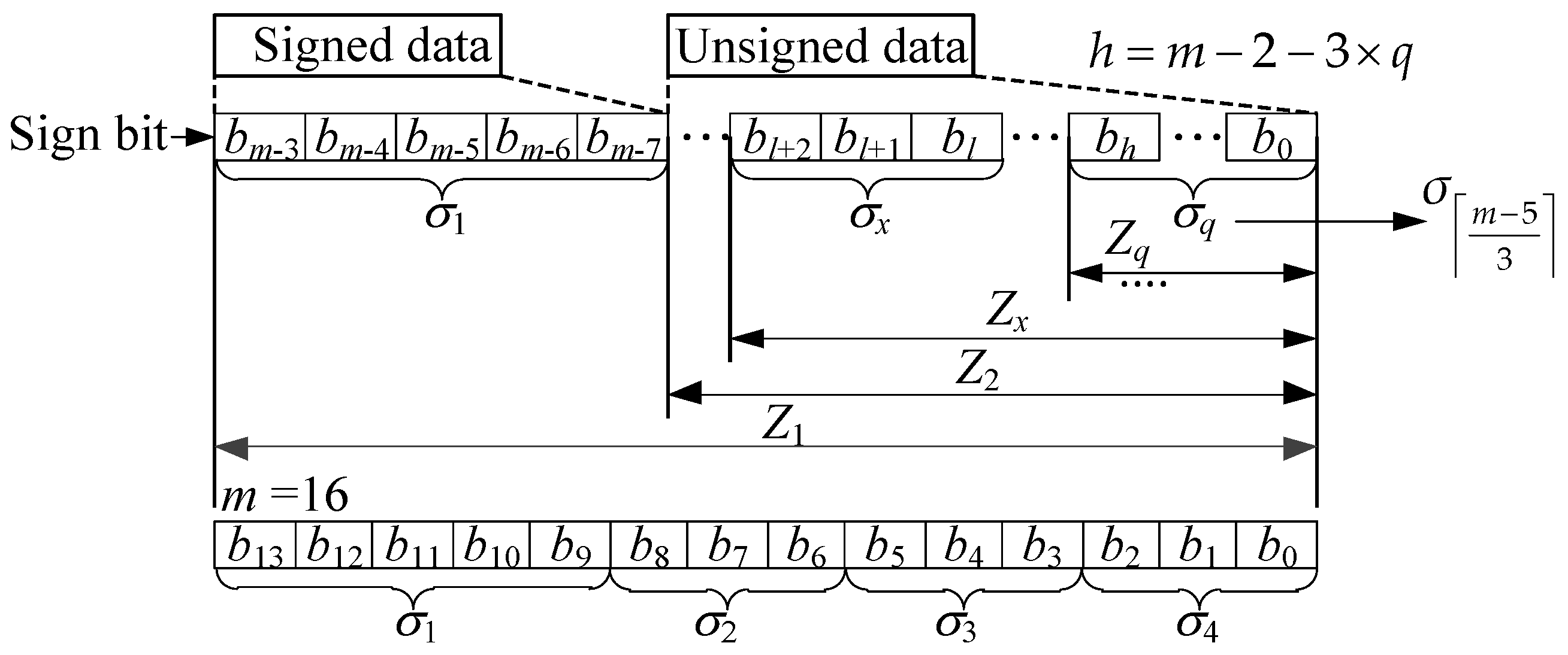
• Compute ${\sigma }_i,i=1,\dots ,q$ by directly fetching bits from ${\mathrm{Z}}_1$ as in Equation (25).
• Compute A and B as in Equation (20) using ${\sigma }_i$ at the third step, all of which are small integers. For example, ${\sigma }_0\in \left[0,2\right]$ is a 2-bit unsigned integer, and ${\sigma }_1\in \left[-8,8\right]$ is a 5-bit signed integer, while ${\sigma }_i\in \left[0,7\right],i=2,3,\cdots q$ is an unsigned integer no greater than 3-bit.

Thus, Equation (17) can be rewritten as

$$\left[\begin{array}{c}A\\ B\end{array}\right]=\left[\begin{array}{c}{A}_n\\ B_n\end{array}\right]=\frac{1}{2^m}\left[\begin{array}{c}{2}^m-\frac{{\sigma }_0}{2^3}\times z_1-\frac{{\sigma }_1}{2^7}\times z_2\\ 2^{\left(m-3\right)}\times {\sigma }_0+z_1\end{array}\right]$$

(29)

Since all ${\sigma }_i$ are small integers, their multiplication computations in Equation (29) can be easily implemented by using shifting and additions.

According to the above deduction for the NR-8 CORDIC algorithm, the implementation of the digital circuit structure of the proposed NR-8 CORDIC algorithm is shown in Figure 4. The contents of the green dashed box can be implemented with a Digital Signal Processing (DSP) module. Therefore, all iterative processes are not required, and thus the NR-8 CORDIC algorithm only takes three clock cycles for computation:

Cycle 1: Fold the angle $\theta \in [0,\pi /2]$ to the range of $\phi \in [0,\pi /12]$, and transform the input variables from $x_0,y_0$ to $x_0^{\prime },y_0^{\prime }$, according to Table 1, Section 3.4 and Figure 4. Compute ${\sigma }_0$, $Z_1$ via rounding $8\phi$ and using the equation of $Z_i=\lfloor z_i\times 2^m\rfloor$ and a three-entry register in Equation (21), respectively.

Cycle 2: Directly fetch the values of ${\sigma }_i$ and $z_i$, $(i=1,2,\cdots q)$ from $Z_1$ as in Equations (25)–(28), respectively, which are substituted to Equation (29) for computing A, B, and meanwhile compensate the amplitude of the variables $x_0^{\prime },y_0^{\prime }$ through the equations $x_0^{″}=K\times x_0^{\prime },y_0^{″}=K\times y_0^{\prime }$.

Cycle 3: Compute the final results $\left[\begin{array}{l}{x}_d\\ y_d\end{array}\right]$ according to Equation (20) and Table 1 by using the multiplier module [18].

4.2. Resource Utilization and Performance Analysis

Here, two comparisons are presented for analyzing resource utilization (RU) and performance as follows.

4.2.1. RU Comparison of Conventional CORDIC Algorithms

The NR-8 CORDIC algorithm and several conventional algorithms are implemented on a Xilinx FPGA (xcku040-ffva1156) including the evaluations of the critical RU, clock latency and power consumption, and these conventional algorithms are R-2, R-4 and R-8 [11,12,13,15]. Note that in the experiments, the 16, 8 and 6-level pipelines are used for R-2, R-4 and R-8 CORDIC cores to achieve the same accuracy, respectively [15].

Table 2. Utilization comparison of the NR-8 CORDIC algorithm with the conventional CORDIC algorithms with 16-bit precision.

Algorithms	CLB LUTs a (242,400)/UT (%)	FF (484,800)/UT (%)	DSPs (1920)/UT (%)	Clock b Latency	Power (Dynamic/Static) (W)
R-2 [11]	1095/0.45	785/0.16	2/0.1	17	0.071/0.479
R-4 [12]	975/0.4	329/0.07	5/0.26	9	0.066/0.478
R-8 [15]	880/0.36	234/0.05	6/0.31	7	0.065/0.478
NR-8	300/0.12	98/0.02	5/0.21	3	0.031/0.478

^a A CLB contains 8 6-input LUTs and 16 flip-flops [19]. ^b The working clock frequency of 250 MHz.

lists RU comparisons of the R-2, R-4 and R-8 CORDIC algorithms with the NR-8 CORDIC algorithm by using a synthesis tool (Vivado 2019.2) (2019.2, Xilinx, San Jose, CA, USA, 2019). The results demonstrate that the proposed NR-8 CORDIC algorithm has advantages over the conventional algorithms in many aspects, such as the RUs of Configurable Logic Block (CLB) Lookup Tables (LUTs), flip-flop (FF), DSPs, clock latency, power consumption and so forth. For example, for a 16-bit precision output, compared with the corresponding parameters of the R-2, R-4 and R-8 CORDIC algorithms in Table 2, the proposed NR-8 algorithm only requires one-half to one-eighth the RU and reduces clock latency to one-half to one-sixth and power consumption to one-half. Then, we implemented the algorithm in Verilog Hardware Description Language (HDL) using a pipelined approach. The place and route tool reports the worst negative slack and the worst hold slack as 0.302 ns and 0.024 ns, respectively, when using a clock frequency of 250 MHz. Compared with the conventional ones, such as the CORDIC IP core (6.0) from Xilinx with 16-bit precision and three iterations, the power of the NR-8 CORDIC algorithm significantly decreases to below 70%, and the proposed algorithm only needs one-third of the flip-flops, though the low power consumption LUTs utilization increases by 43%.

4.2.2. Performance Comparison of Newly Developed CORDIC Algorithms

The comparisons of performance of the newly developed algorithms [12,13,14,15] with the NR-8 CORDIC algorithm are shown in

Table 3. Performance comparison of newly developed CORDIC algorithms with m-bit precision.

Algorithms	Conventional CORDIC [12,13,15]			High-Performance R-4 [14]	Low-Latency Hybrid (LLH) [16]	High-Performance/Low-Latency [17]	Proposed NR-8 CORDIC
	R-2	R-4	R-6
Iterations	m + 1	(1/2)m	(3/8)m	m/2	(3/8)m+1	-	0
Complexity a	O(2m)	O(2m)	O((15/8)m)	O(m)	O(3m)	16 Adders/28 Adders (m = 16)	$O(2^{\lceil \frac{m-5}{3}\rceil })$
Timing (Critical path) b	Tadd/sub	Tadd/sub	Tadd/sub	Tadd/sub	2Tadd/sub	2Tadd/sub	2Tadd/sub
Latency (m = 16)	17	9	7	8	6	68TFA/26TFA c	3

^a Base on analysis of critical rotator module. O(●): order in terms of full adders. - not reported. ^b Tadd/sub means Adder/subtractor delay. ^c T_FA means a full adder delay.

. The conventional Radix-X CORDIC algorithms, such as the R-2 CORDIC with m-bit precision, require m iterations. Normally, the number of iterations decreases as the number of X in Radix-X increases, and the complexity and timing (critical path) of the algorithms are almost unchanged. The high-performance R-4 CORDIC algorithm [14] requires m/2 iterations, O(m) complexity and low latencies. The low-latency hybrid (LLH) CORDIC algorithm [16] requires 3m/8 + 1 iterations and more complexity O(3m). Although the high performance/low-latency (HPLL) CORDIC algorithm [17] has low latency, this algorithm is not conducive to pipeline optimization to improve the speed, owing to the inherent iterative structure.

For the NR-8 CORDIC algorithm, when the precision is less than 24 bits, complexity is less than $O(2^q)$, $q=\lceil \frac{23-5}{3}\rceil =6$, and ${\sigma }_i$ has only seven types ($i\in \{0,1,2,3,4,5,6\}$). Thus, Equations (15) and (26) are rewritten as

$$\{\begin{array}{l}F\left(m\right)=\left|a_{i_1}{a}_{i_2}\dots a_{i_m}\right|, (i_1,i_1,\dots i_m)\in \left\{0,1,2,3,4,5,6\right\}, 0\le m\le 6\\ a_i=\{\begin{array}{ll}{\sigma }_0{2}^{-3},\hfill & i=0\hfill \\ {\sigma }_i{2}^{-\left(4+3i\right)},\hfill & i=1,2,3,4,5,6\hfill \end{array}\end{array}$$

(30)

We can make a conclusion from Equation (30) that when $4\le m\le 6$, if and only if $a_{i_1}{a}_{i_2}\dots a_{i_m}$ = $a_0{a}_1{a}_2{a}_3$, the maximum of $F\left(m\right)$ is given as

$$\mathrm{MAX}{\left(F\left(m\right)\right)|}_{4\le m\le 6}=\left|a_0{a}_1{a}_2{a}_3\right|=\left|\frac{{\sigma }_0}{2^3}\times \frac{{\sigma }_1}{2^7}\times \frac{{\sigma }_2}{2^{10}}\times \frac{{\sigma }_3}{2^{13}}\right|\le \frac{2\times 8\times 7\times 7}{2^{33}}\le \frac{1}{2^{23}}$$

(31)

Apparently, when the NR-8 CORDIC algorithm requires 23-bit precision, the following approximations are produced: ${F\left(m\right)|}_{4\le m\le 6}\approx 0$ and ${f_a\left(C_n^m\right)|}_{4\le m\le 6}\approx 0$ ($f_a\left(C_n^m\right)$ from Equation (14)). The most time-consuming path is attributed to the computation of variables A, B. According to the above analysis and Equation (13), A, B can be simplified as

$$\left[\begin{array}{c}A\\ B\end{array}\right]=\left[\begin{array}{c}{A}_n\\ B_n\end{array}\right]=\frac{1}{2^m}\left[\begin{array}{c}{2}^m-\frac{{\sigma }_0{z}_1}{2^3}-\frac{{\sigma }_1{z}_2}{2^7}-\frac{{\sigma }_2{z}_3}{2^{10}}-\frac{{\sigma }_3{z}_4}{2^{13}}\\ 2^{\left(m-3\right)}\times {\sigma }_0+z_1-\frac{{\sigma }_0{\sigma }_1{z}_2}{2^{10}}-\frac{{\sigma }_0{\sigma }_2{z}_3}{2^{13}}\end{array}\right]$$

(32)

Equation (32) can be realized by two-clock latency in the pipeline. Therefore, only four-clock latency is required for the NR-8 CORDIC algorithm with 23-bit precision, and the complexity is less than $O(15)$. For instance, compared with the 10-clock latency required for $\frac{3}{8}\times 23+1\approx 10$ iterations using the LLH CORDIC algorithm [16], the clock latency of the NR-8 CORDIC algorithm significantly decreases to less than 50%, which needs only the four-clock latency.

4.3. Error Analysis

4.3.1. Comparisons with Low-Latency Hybrid (LLH) CORDIC

According to the literature [16], the simulation has been performed to compute the cosine and sine functions for the angles $\theta$, ranging from 0 to $\pi /2$ in the step of $\pi /500$. ${\sigma }_0,{\sigma }_1,z_1,z_2$ come from Equations (25)–(28). $x_0^{\prime },y_0^{\prime }$ come from Table 1 and Figure 4. For m-bit precision, the critical descriptive codes for the NR-8 CORDIC algorithm are described in Algorithm 1.

Algorithm 1. The descriptive codes of the NR-8 CORDIC.

$x_0=2^m,y_0=0;$

$\begin{array}{l}A=2^m-fix\left(({\sigma }_0\times z_1)/2^3\right)-fix\left(({\sigma }_1\times z_2)/2^7\right);\\ B=2^{(m-3)}\times {\sigma }_0+z_1;\end{array}$

$K=2^{15}-2^8\times {\sigma }_0^2+3\times {\sigma }_0^4-{\sigma }_1^2;$

$\begin{array}{l}{x}_0^{″}=fix\left((x_0^{\prime }\times K)/2^{15}\right);\\ y_0^{″}=fix\left((y_0^{\prime }\times K)/2^{15}\right);\end{array}$

$\begin{array}{l}{x}_d=A\times x_0^{″}-B\times y_0^{″};\\ y_d=sign\_sel(A\times y^{″}+B\times x_0^{″});\end{array}$

$\begin{array}{l}\mathrm{NR}8\cos =\mathrm{R}\cos /2^{2m};\\ \mathrm{NR}8\sin =\mathrm{R}\sin /2^{2m};\end{array}$

Two functions, $\cos \theta$ and $\sin \theta$, are produced by using standard functions from MATLAB, and the amplitude errors are described as

$$\{\begin{array}{c}{\mathsf{\delta }}_{NR8c}=\left|\mathrm{NR}8\cos -\cos \theta \right|\\ {\mathsf{\delta }}_{NR8s}=\left|\mathrm{NR}8\sin -\sin \theta \right|\end{array}$$

(33)

Figure 5a shows the values of cosine and sine produced by the NR-8 CORDIC algorithm. Figure 5b,c compare the errors for the cosine and sine functions between the NR-8 CORDIC and the LLH CORDIC [16] with 16-bit precision, respectively. The symbols of ${\mathsf{\delta }}_{NR8c}$ and ${\mathsf{\delta }}_{NR8s}$ stand for the absolute differences of cosine and sine between the computed value from the NR-8 CORDIC and the theoretical value produced from MATLAB functions, respectively. Similarly, the symbols of ${\mathsf{\delta }}_{LLHc}$ and ${\mathsf{\delta }}_{LLHs}$ denote the absolute differences of cosine and sine between the computed value from the LLH CORDIC [16] and the theoretical value produced from MATLAB functions, respectively. It is found that the maximum errors are ${\mathrm{MAX}(\mathsf{\delta }}_{LLHc})$ = 8.04 × 10⁻⁴ and ${\mathrm{MAX}(\mathsf{\delta }}_{LLH\mathrm{s}})$ = 5.50 × 10⁻⁴ for the cosine and sine functions, respectively, in the literature [16], which significantly decrease down to $\mathrm{MAX}({\mathsf{\delta }}_{NR8c})$ = 9.20 × 10⁻⁵ and $\mathrm{MAX}({\mathsf{\delta }}_{NR8s})$ = 9.01 × 10⁻⁵ in the NR-8 CORDIC algorithm, respectively, thus indicating that the proposed NR-8 algorithm has high precision. Moreover, according to our analyses for the structures of the two algorithms, similar results should be obtained for the 24-bit precision.

4.3.2. Comparison of Conventional CORDIC Algorithms

Here, we analyze the computation errors $\cos \theta$ and $\sin \theta$, as calculated by the R-2, R-4, R-8 and NR-8 CORDIC algorithms. When $x_0=2^M-1,y_0=0$ ($M\le 16$) and a series of angles $\theta$ from 0 to 90° with angle steps of 1, 0.1, 0.01 and 0.001° are used, the values of cos$\theta$ and sin$\theta$ are computed by the algorithms above using FPGA and simulated by ModelSim SE (10.6e). The errors can be calculated by differing the above values from those computed by MATLAB using float-point computation and rounding to M-bit integers. Figure 6 shows the maximum absolute errors (MAE) for the cos$\theta$ and sin$\theta$ functions, which are denoted as ${\delta }_{\cos }(x),{\delta }_{\sin }(x)$ (steps = 1, 0.1, 0.01, 0.001°), and the corresponding root mean squared errors (RMSE) are shown in Figure 7. The proposed algorithm was simulated by ModelSim SE and MATLAB fixed-point processing, and verified by using the FPGA. We obtained the same results, indicating that the algorithm is feasible in engineering implementation.

From Figure 6 and Figure 7, it is found that the proposed NR-8 CORDIC algorithm is the most sensitive to the bit width $M$, and as the $M$ value decreases, both the MAE and RMSE values decrease sharply. Even though the value of $M$ equals 15 or 16, the MAE and RMSE values of the proposed NR-8 CORDIC algorithm are almost as small as those of the other algorithms. Note that when the value of $M$ is smaller than 15, the MAE and RMSE values of the NR-8 CORDIC algorithm are much smaller than those of the other algorithms. As a consequence, the overall MAE and RMSE values of the NR-8 CORDIC algorithm are relatively small in comparison with the conventional algorithm. In addition, the angle step functions have less influence on the MAE and RMSE values of the proposed NR-8 CORDIC algorithm than the other conventional algorithms. Specifically, both the MAE and RMSE values for the cosine function calculated using the NR-8 CORDIC algorithm are almost the same as the corresponding values for the sine function, indicating that the outputs of the cosine and sine functions are mostly orthogonal. However, for the other conventional algorithm, the orthogonality is relatively weak. Moreover, we made the statistical test more than 1000 times and found out that all of the MAEs and RMSEs for the cosine and sine functions are in the corresponding ranges described above, indicative of the significance of our proposed method. Therefore, we make a conclusion that the NR-8 CORDIC algorithm developed in this paper has lower clock latency, less complexity and less consumed power, allowing it to have higher efficiency than other algorithms, which provides a potential application in real-time systems such as radar digital beamforming.

5. Application of the NR-8 CORDIC Algorithm to DBF

The diagram of the DBF mode for the MIMO millimeter wave radar is shown in Figure 8. The interface of the FPGA and ADC is the LVDS bus, and the phase shift Transmission (TX) is implemented by the FPGA, which transmits commands to AWR1243 registers through the SPI bus. The desired steering angles are defined to be ${\beta }_1,{\beta }_2,\cdots {\beta }_n$ for n TX antennas. The received I, Q complex data from ADC for each Reception (RX) channel go through a DSP module that includes the range and Doppler FFT. RX DBF is performed to steer the RX beam towards the same ${\beta }_i$. After the corresponding phase delay, the echoes are summed to achieve a beamforming [20,21].

According to Equation (1), if the input vector $\left[\begin{array}{c}{x}_0\\ y_0\end{array}\right]$ is not a constant vector and the input angle $\theta$ is a desired value, the vector $\left[\begin{array}{c}{x}_0\\ y_0\end{array}\right]$ will produce the phase shift by the $\theta$. Thus, we can realize the beam delay of the desired steering angles according to the NR-8 CORDIC algorithm. In Figure 4, if $x_0,y_0$ are replaced by I, Q complex data, respectively, and the angle $\theta$ is replaced by ${\beta }_i$, the output values $x_d,y_d$ will be obtained as the corresponding beam delay vector.

In this section, the NR-8 CORDIC algorithm is applied to the phase delay for DBF on a 77 GHz MIMO millimeter wave radar system empowered by TI AWR1243 chips. The experimental device of DBF for the MIMO millimeter wave radar is shown in Figure 9. The related parameters are as follows: the sampling rate f_s = 4 MHz, the bandwidth bw = 1120 MHz and the sampling points N = 16, where the bandwidth refers to the bandwidth of the radio frequency. However, if the baseband signal is implemented by the radar chip with digital down converters, the frequency will be reduced from 1120 MHz to less than 1 MHz. Therefore, we can use fs = 4 MHz for sampling. The sample points are listed below: $\left\{\mathrm{I},Q\right\}$ = {−168 − 64i, −60 − 224i, 224 − 88i, 148 + 84i, 52 + 196i, −164 + 60i, −36 − 132i, 276 − 4i, 128 + 164i, −84 + 284i, −188 + 56i, 12 − 168i, 128 + 40i, −64 + 264i, −236 + 104i, −132 − 204i}. A corner reflector is placed in front of the radar at a distance of 3 m and an azimuth of 20°.

One echo (I/Q) is taken for phase shift angle $\theta$ from 1.5° to 15° with a 1.5° step, producing 10 phases. Let $x_0=I$ and $y_0=Q$ in Figure 4. The phase shift effects are shown in Figure 10, where the red and green lines represent I and Q signals, respectively. The 1st and 10st symbols in the illustration represent beam delays of 1.5° (beam_1) and 15° (beam_10), respectively. FFT transformation is applied to each beam, and the phase errors are listed in

Table 4. Phase errors of FFT transform.

Beams	(I,Q)	Beam_1	Beam_2	Beam_3	Beam_4	Beam_5	Beam_6	Beam_7	Beam_8	Beam_9	Beam_10
$p$(°)	−129.305	−127.807	−126.354	−124.814	−123.361	−121.804	−120.241	−118.812	−117.344	−115.858	−114.290
${\tilde{\Delta }}_p$(°)	0	1.498	2.951	4.491	5.944	7.501	9.064	10.493	11.961	13.447	15.015
${\Delta }_p$(°)	0	1.5	3.0	4.5	6.0	7.5	9.0	10.5	12.0	13.5	15.0
${\delta }_{\Delta p}$(°)	0	−0.002	−0.049	−0.009	−0.056	0.001	0.064	−0.007	−0.039	−0.053	0.015

. The variables $p$, ${\tilde{\Delta }}_p$, ${\Delta }_p$ and ${\delta }_{\max \_p}$ ${\delta }_{\max \_p}$ are described as follows:

• $p={\mathrm{ANGLE}\left(\mathrm{FFT}(beam\_n or \left\{\mathrm{I},\mathrm{Q}\right\})\right)|}_{PEAK}$, the phase angle of the nth delay beam or $\left\{\mathrm{I},Q\right\}$.
• ${\tilde{\Delta }}_p={\mathrm{ANGLE}\left(\mathrm{FFT}(beam\_n )\right)|}_{PEAK}-{\mathrm{ANGLE}\left(\mathrm{FFT}(\left\{\mathrm{I},Q\right\})\right)|}_{PEAK}$, the phase difference between the nth delay beam and the original echo $\left\{\mathrm{I},Q\right\}$.
• ${\Delta }_p$ = the desired steering angles.
• ${\delta }_{\Delta p}={\tilde{\Delta }}_p-{\Delta }_p$ = the error of the phase shift.

where n = 1, 2, ⋯, 10 and the functions $\mathrm{FFT}(beam\_n)$ and $\mathrm{FFT}(beam\_1)$ represent the FFT transformation of the nth delay beam and the first delay beam, respectively. Then, the phase differences corresponding to the peak values of the spectral lines are obtained. In Table 4, the small value of the inequality, $\left|{\delta }_{\Delta p}\right|<{0.064}^{°}$, assures that the NR-8 CORDIC algorithm can be applied in real-time systems like radar digital beamforming with a high precision of the phase shift.

Overall, our algorithm is mainly based on noniterative methods, whereas the majority of the conventional algorithms are based on the iterative methods, and thus our algorithm is low latency and high efficiency for the high precision output. As for the normal CORDIC algorithm, the increase of the computational complexity means the change of the important module, with the increase of precision and, in detail, the adders required for fulfilling the same task such as a task in Figure 4, will increase. For example, the number of adders that are used to get the values of A_n and B_n from Equation (13) will increase with the increase of the computational complexity. As for the R-2 CORDIC algorithm, the m iterators are required for achieving the m-bit precision output, each of which needs an adder and a subtractor; thus the computational complexity can be expressed by a term of O(m). Meanwhile, the data we achieved are based on the statistical test for several trials, and the results are found to be very reliable with a relatively low error, thus indicating the NR-8 CORDIC algorithm is able to be applied in these fields with low latency and high efficiency.

6. Conclusions

The proposed NR-8 CORDIC algorithm has low latency, low complexity and low RU, in comparison with the conventional R-X CORDIC and some newly developed CORDIC algorithms. In particular, when the m-bit precision is less than 24-bit, this algorithm has great advantages, e.g., the clock latencies can be reduced to 4 from 10 with much lower complexity. This algorithm adopts the narrow input angle range to obtain a high speed for calculations, and it uses the output uniform formula to efficiently compute the sine and cosine functions or the phase shift in a noniterative fashion. Therefore, this algorithm is of great value in time-critical applications, such as DBF, robot controllers, FFT transformation, signal modulation and demodulation, recently developed rapid convolutional neural networks (CNNs) [22,23] and so on. We anticipate that the algorithm will provide a higher precision, lower complexity and lower clock latency after further optimization in the future.

References

1. Fang, L.; Xie, Y.; Li, B.; Chen, H. Generation scheme of chirp scaling phase functions based on floating-point CORDIC processor. J. Eng. 2019, 2019, 7436–7439. [Google Scholar] [CrossRef]
2. Vyas, P.; Vachhani, L. CORDIC-Based Azimuth Calculation and Obstacle Tracing via Optimal Sensor Placement on a Mobile Robot. IEEE/ASME Trans. Mechatron. 2016, 21, 2317–2329. [Google Scholar] [CrossRef]
3. Wong, C.C.; Liu, C.C. FPGA realisation of inverse kinematics for biped robot based on CORDIC. Electron. Lett. 2013, 49, 332–334. [Google Scholar]
4. Lee, H.; Oh, K.; Cho, M.; Jang, Y.; Kim, J. Efficient Low-Latency Implementation of CORDIC-Based Sorted QR Decomposition for Multi-Gbps MIMO Systems. IEEE Trans. Circuits Syst. II Express Brief 2018, 65, 1375–1379. [Google Scholar] [CrossRef]
5. Jun, M.; Parhi, K.K.; Deprettere, E.F. Annihilation-Reordering Look-Ahead Pipelined CORDIC-Based RLS Adaptive Filters and Their Application to Adaptive Beamforming. IEEE Trans. Signal Process. 2000, 48, 2414–2431. [Google Scholar] [CrossRef]
6. Nikolov, S.I.; Jensen, J.A.; Tomov, B.G. Fast parametric beamformer for synthetic aperture imaging. IEEE Trans. Ultrason. Ferroelectr. Freq. Control 2008, 55, 1755–1767. [Google Scholar] [CrossRef] [PubMed] [Green Version]
7. Pilato, L.; Fanucci, L.; Saponara, S. Real-Time and High-Accuracy Arctangent Computation Using CORDIC and Fast Magnitude Estimation. Electronics 2017, 6, 22. [Google Scholar] [CrossRef] [Green Version]
8. Lakshmi, B.; Dhar, A.S. CORDIC architectures: A survey. VLSI Des. 2010, 2010, 794891. [Google Scholar] [CrossRef]
9. Ylostalo, J. Function approximation using polynomials. IEEE Signal Process. Mag. 2006, 23, 99–102. [Google Scholar] [CrossRef]
10. Ercegovac, M.D.; Lang, T.; Muller, J.M.; Tisserand, A. Reciprocation, square root, inverse square root, and some elementary functions using small multipliers. IEEE Trans. Comput. 2000, 49, 628–637. [Google Scholar]
11. Volder, J.E. The CORDIC Trigonometric Computing Technique. IEEE Trans. Electr. Comput. 1959, 8, 330–334. [Google Scholar] [CrossRef]
12. Meher, P.K.; Valls, J.; Juang, T.B.; Sridharan, K.; Maharatna, K. 50 Years of CORDIC: Algorithms, Architectures, and Applications. IEEE Trans. Circuits Syst. I Regul. Pap. 2009, 56, 1893–1907. [Google Scholar] [CrossRef] [Green Version]
13. Maharatna, K.; Banerjee, S.; Grass, E.; Krstic, M.; Troya, A. Modified virtually scaling-free adaptive CORDIC rotator algorithm and architecture. IEEE Trans. Circuits Syst. Video Technol. 2005, 15, 1463–1474. [Google Scholar]
14. Antelo, E.; Villalba, J.; Bruguera, J.D.; Zapata, E.L. High performance rotation architectures based on the radix-4 CORDIC algorithm. IEEE Trans. Comput. 1997, 46, 855–870. [Google Scholar] [CrossRef] [Green Version]
15. Rudagi, J.; Subbaraman, S. Comparative Analysis of Radix-2, Radix-4, Radix-8 CORDIC Processors. In Proceedings of the 2017 International Conference on Inventive Computing and Informatics (ICICI), Coimbatore, India, 23–24 November 2017; pp. 378–382. [Google Scholar]
16. Shukla, R.; Ray, K. Low latency hybrid CORDIC algorithm. IEEE Trans. Comput. 2014, 63, 3066–3078. [Google Scholar] [CrossRef]
17. Wu, C.S.; Wu, A.Y.; Lin, C.H. A High-Performance/Low-Latency Vector Rotational CORDIC Architecture Based on Extended Elementary Angle Set and Trellis-Based Searching Schemes. IEEE Trans. Circuits Syst. II Analog Digit. Signal Process. 2003, 50, 589–601. [Google Scholar]
18. DSP48 Macro v3.0, Xilinx Inc., USA. 2015. Available online: https://www.xilinx.com/support/documentation/ip_documentation/xbip_dsp48_macro/v3_0/pg148-dsp48-macro.pdf (accessed on 12 August 2020).
19. UltraScale Architecture Configurable Logic Block User Guide. Xilinx Inc., USA. 2017. Available online: https://www.xilinx.com/support/documentation/user_guides/ug574-ultrascale-clb.pdf (accessed on 12 August 2020).
20. Fischman, M.A.; Le, C. Digital beamforming developments for the joint NASA/Air Force Space Based Radar. In Proceedings of the IGARSS 2004, 2004 IEEE International Geoscience and Remote Sensing Symposium, Anchorage, AK, USA, 20–24 September 2004; pp. 687–690. [Google Scholar]
21. Lialios, D.I.; Ntetsikas, N.; Paschaloudis, K.D.; Zekios, C.L.; Georgakopoulos, S.V.; Kyriacou, G.A. Design of True Time Delay Millimeter Wave Beamformers for 5G Multibeam Phased Arrays. Electronics 2020, 9, 1331. [Google Scholar] [CrossRef]
22. Cao, Y.X.; Xiao, W.A.; Jia, J. A Cordic-based Acceleration Method on FPGA for CNN Normalization layer. In Proceedings of the 2020 International Conference on High Performance Big Data and Intelligent Systems (HPBD&IS), Shenzhen, China, 23 May 2020. [Google Scholar]
23. Parmar, Y.; Sridharan, K. A Resource-Efficient Multiplierless Systolic Array Architecture for Convolutions in Deep Networks. IEEE Trans. Circuits Syst. II Express Brief 2020, 67, 370–374. [Google Scholar] [CrossRef]
Figure 1. The CORDIC vector rotation model.
Electronics 09 01521 g001
Figure 2. Decreasing of F(m) as m or S(m) increases.
Electronics 09 01521 g002
Figure 3. The architectures of the variable σ i and the variable Z i ( Z i = z i × 2 m ).
Electronics 09 01521 g003
Figure 4. The architecture diagram of the NR-8 CORDIC algorithm on an FPGA. * The multipliers can be optimized as shifters and adders.
Electronics 09 01521 g004
Figure 5. (a) The curves of cosine and sine computed by the NR-8 CORDIC algorithm. (b) Comparison of errors for cosine between the NR-8 and the LLH CORDIC with 16-bit precision. (c) Comparison of errors for sine between the NR-8 and the LLH CORDIC with 16-bit precision.
Electronics 09 01521 g005
Figure 6. The relations between maximum absolute errors (MAEs) and the input bit width M of the NR-8, R-8, R-4 and R-2 CORDIC algorithms. The angles θ change from 0 to 90° in steps of 1, 0.1, 0.01 and 0.001°.
Electronics 09 01521 g006
Figure 7. The relations between root mean squared errors (RMSEs) and the input bit width M of the NR-8, R-8, R-4 and R-2 CORDIC algorithms. The angles θ change from 0 to 90° in steps of 1, 0.1, 0.01 and 0.001°.
Electronics 09 01521 g007
Figure 8. The diagram of digital beamforming (DBF) mode for the MIMO millimeter wave radar.
Electronics 09 01521 g008
Figure 9. The experimental device of DBF for the MIMO millimeter wave radar.
Electronics 09 01521 g009
Figure 10. The effects of the phase shift showing the partial amplification of delay beams.
Electronics 09 01521 g010