Expedited Globalized Antenna Optimization by Principal Components and Variable-Fidelity EM Simulations: Application to Microstrip Antenna Design

Abstract

Parameter optimization, also referred to as design closure, is imperative in the development of modern antennas. Theoretical considerations along with rough dimension adjustment through supervised parameter sweeping can only yield initial designs that need to be further tuned to boost the antenna performance. The major challenges include handling of multi-dimensional parameter spaces while accounting for several objectives and constraints. Due to complexity of modern antenna topologies, parameter interactions are often involved, leading to multiple local optima as well as difficulties in identifying decent initial designs that can be improved using local procedures. In such cases, global search is required, which is an expensive endeavor, especially if full-wave electromagnetic (EM) analysis is employed for antenna evaluation. This paper proposes a novel technique accommodating the search space exploration using local kriging surrogates and local improvement by means of trust-region gradient search. Computational efficiency of the process is achieved by constructing the metamodels over appropriately defined affine subspaces and incorporation of coarse-mesh EM simulations at the exploratory stages of the optimization process. The resulting framework enables nearly global search capabilities at the costs comparable to conventional gradient-based local optimization. This is demonstrated using two antenna examples and comparative studies involving multiple-start local tuning.

1. Introduction

Full-wave electromagnetic (EM) simulations play a crucial role in the design of modern antennas. Their employment is imperative to secure evaluation reliability, especially for situations where simpler (e.g., analytical or network equivalent) models are not available or lack accuracy. The examples include compact antennas with tightly arranged layouts [1], the presence of connectors and radomes [2], as well as mutual coupling of radiators [3]. At the same time, the necessity of handling several performance figures (e.g., antenna reflection, gain, axial ratio, footprint area) and carrying out the tuning process over multi-dimensional parameter spaces leads to a more and more widespread utilization of numerical optimization routines. Notwithstanding, the computational costs of EM-driven design may be considerable even in the case of local optimization [4], let alone global search procedures which might be required when sufficiently good initial designs are not available or the problem at hand is a multi-modal one [5]. Common examples include design of compact antennas [6], wideband-antennas [7,8,9], array pattern synthesis [10], or optimization of MIMO systems [11].

Population-based metaheuristics belong to the most widely used global optimization methods [12,13,14,15,16,17,18,19,20], typically mimicking certain biological [12] or social phenomena [13]. Within these algorithms, it is the cooperation and exchange of information between individuals (agents, particles, etc.) that permits design space exploration, identification of the promising regions, and escaping from local minima. Some popular techniques include not only genetic algorithms [14], particle swarm optimizers [15], differential evolution [16], and firefly algorithm [17] but also numerous recent variations, often being slight variations of the existing methods featuring fancy names (e.g., Strawberry Algorithm [18], Monarch Butterfly Algorithm [19], Bat Flower Pollination [20]). Unfortunately, the CPU cost of these algorithms is very high due to processing sets of candidate solutions in each iteration, which may be prohibitive when directly handling EM simulation models. A possible way of alleviating this issue are machine learning methods combining metaheuristics with iterative construction of fast surrogate models [21,22], incorporation of gradient-based procedures [23], or variable-fidelity simulations [24]. Other methods include multiple start local optimization or the Taguchi method that involves experimental design using orthogonal arrays [25]. Nevertheless, these variations are of rather limited popularity with mainstream metaheuristics remaining—despite their high cost—the most popular solution approaches for global optimization in high-frequency design.

Having in mind that the antenna optimization process needs to be carried out at the level of full-wave EM analysis in most situations, the development of more efficient procedures that exhibit—to a certain extent—global search capabilities while offering practically acceptable computational cost seems to be of paramount importance. This paper presents an algorithm for globalized design optimization of antennas. Its key components include parameter space exploration using local kriging surrogates and trust-region gradient search for local tuning. The kriging metamodels are established over low-dimensional affine subspaces spanned by the most relevant directions corresponding to the maximum variability of antenna characteristics (averaged over the frequency range of interest). The latter are established using principal component analysis of antenna response Jacobians. To further reduce the cost of the optimization process, low-fidelity (coarse-mesh) EM model is employed at the exploration stage, whereas the local tuning replaced costly finite differentiation by rank-one Broyden formula for sensitivity updates. The combination of variable-fidelity surrogate-assisted exploration and expedited trust-region algorithm enables quasi-global search capability at the cost comparable to local optimization. This is demonstrated using two antenna examples, a wideband monopole and a triple-band uniplanar dipole. The efficacy of the proposed approach is further validated by comprehensive statistical studies and benchmarking against multiple-start local search.

2. Variable-Fidelity Globalized Optimization Using Principal Components and Kriging Surrogates

This section recalls the formulation of the antenna optimization task, discusses variable-fidelity simulation models, and explains the basic components of the proposed globalized search procedure. The entire framework is subsequently summarized, also in a form of the flow diagram. Numerical verification of the method and benchmarking can be found in Section 3.

2.1. Formulation of Design Optimization Task

The output of the EM-simulation model of the antenna at hand will be denoted as R_f(x) and represents any relevant characteristics (e.g., reflection or gain versus frequency). Here, x = [x₁ … x_n]^T ϵ X is a vector of adjustable variables, typically, geometry parameters. The subscript f is to distinguish the high-fidelity (or fine) model to be optimized, from an auxiliary low-fidelity (coarse) one which will be discussed in Section 2.2. The parameter space X is delimited by the lower and upper bounds l = [l₁ … l_n]^T and u = [u₁ … u_n]^T, i.e., we have l_k ≤ x_k ≤ u_k, k = 1, …, n.

The design quality is quantified using a scalar cost function U, which depends on a particular problem to be solved. One of the most common tasks is minimization of the antenna reflection over a frequency range of interest F, in which case, we may define U(R_f(x)) = U(S_11.f(x,f)) = max{f ϵ F: |S_11.f(x,f)|}.

Given U, the optimization problem is then defined as

$$x^{*}=\arg \underset{x\in X}{\min }U(R_f(x))$$

(1)

In general, the problem one can be constrained, i.e., additional conditions of the form g_k(x) ≤ 0, k = 1,…, N_ineq (inequality constraints) and h_k(x) = 0, k = 1, …, N_eq (equality constraints) may be imposed. In the following, we focus on box-constrained domain as defined above.

2.2. Variable-Fidelity Simulation Models

Utilization of variable-fidelity models is one of widely used means to accelerate all sort of EM-driven design procedures. In the case of antennas, low-fidelity models, here denoted as R_c, are normally obtained from coarse-mesh simulation [26], which might be supplemented by other simplifications of the computational models (e.g., the use of discrete sources rather than waveguide ports, ignoring dielectric and metal losses, etc.) [27]. When applied to local search using methods such as space mapping [28], response correction [29], or feature-based optimization [30], good correlation between the low- and high-fidelity model is of paramount importance to ensure reliability of the optimization process [31]. This imposes limitation on the coarseness of the low-fidelity model. In this work, however, the R_c will be used at the exploratory stages of the search process, where the main objective is to identify the promising regions of the parameter space. In this context, excellent model correlations are not critical, so that coarser models may be potentially used to improve the computational efficiency of the optimization process but without compromising the design quality. This aspect will be investigated in Section 3. Figure 1 shows the high- and low-fidelity model reflection responses at the selected designs for the two antenna structures considered later in the paper as the test cases. It can be observed that both low-fidelity models retain certain level of correlation with the high-fidelity one, but the coarsest version would be definitely insufficient for local optimization purposes.

2.3. Principal Components. Affine Subspace for Exploration Stage

The primary prerequisite for design space exploration, i.e., identification of the promising regions that might contain high-quality designs, is that it does not incur significant computational expenses. In this work this is achieved in two ways: (i) using low-fidelity EM models (cf. Section 2.2) and (ii) conducting exploration over the selected, low-dimensional affine subspaces, spanned by the principal components of the antenna response Jacobians.

We denote by x⁽ⁱ⁾ the current design obtained as a result of the i − 1 iteration of the optimization algorithm. For the sake of maintaining low cost of the process, it is reasonable to restrict the exploration to directions that correspond to the maximum variability of the antenna responses. Here, such directions are found using the Jacobian matrix J_R(x⁽ⁱ⁾). Assuming the most typical situation, i.e., that the output of the high-fidelity EM model R_f(x⁽ⁱ⁾) represents frequency characteristic (e.g., antenna reflection) over a discrete set of frequencies f_k, k = 1, …, m, we have R_f(x⁽ⁱ⁾) = [R_f(x⁽ⁱ⁾,f₁) … R_f(x⁽ⁱ⁾,f_m)]^T and

$$J_R(x^{(i)})={\left[{\nabla }_1^{}(x^{(i)})\dots {\nabla }_m^{}(x^{(i)})\right]}^T$$

(2)

The gradients in (2) are defined as

$${\nabla }_k^T(x^{(i)})=\left[\frac{\partial R_f(x^{(i)},f_k)}{\partial x_1}\dots \frac{\partial R_f(x^{(i)},f_k)}{\partial x_n}\right]$$

(3)

Note that the vector ∇_k(x⁽ⁱ⁾) determines the direction of the maximum antenna response variability at the frequency f_k. In order to get an idea of the overall response variability, i.e., over the entire frequency range of interest, we consider the set {∇_k(x⁽ⁱ⁾)}_{k = 1,..,m} and its covariance matrix [32]

C = (m – 1)^–1S^TS

(4)

where

S = |J_R| –1μ^T

(5)

In (5), |J_R| is a matrix of the gradient moduli, μ = [μ₁ … μ_n]^T represents the means of the gradient moduli, and 1 stands for the m × 1 vector of all ones. We have [32]

$$C=VE{V}^{-1}$$

(6)

where V = [v₁ … v_n] is a matrix of eigenvectors and E is a diagonal matrix of the corresponding eigenvalues λ_i. The eigenvalues are assumed to be arranged in a descending order, i.e., λ₁ ≥ … ≥ λ_n. They represent the variances of the observable set {∇_k(x⁽ⁱ⁾)}_{k = 1,..,m} projected onto one-dimensional subspaces spanned by the corresponding eigenvectors. In plain words, the eigenvectors v_k determine (in the descending order) the directions of the maximum antenna response variability averaged over the frequency range of interest. This becomes a basis for setting up the affine subspace S⁽ⁱ⁾, which will be subsequently used to carry out design space exploration. The subspace is defined as [32]

$$S^{(i)}=x^{(i)}+{\displaystyle {\sum }_{j=1}^{N_s}{a}_j{v}_j}$$

(7)

where a_j are real-valued coefficients. As mentioned before, in practice, a small number of directions is used, e.g., N_s = 2 in order to reduce the computational cost of the exploration stage, in particular, the construction and optimization of an auxiliary kriging interpolation metamodel (cf. Section 2.4).

2.4. Surrogate Model Construction

Another component of the proposed globalized optimization is a fast surrogate model R_s⁽ⁱ⁾ established over the subspace S⁽ⁱ⁾ (Section 2.3). More specifically, the surrogate is rendered within the union S⁽ⁱ⁾ ∩ X using kriging interpolation [33]. The training data is allocated using sequential sampling with the primary objective being the improvement of the model predictive power. The design of experiment scheme works as follows:

• Use Latin Hypercube Sampling (LHS) [34] to distribute the initial set of N_init training samples x_t^(k);
• If card({x_t^(k)}) < N₁, find a new sample that maximizes the mean square error (MSE) [35] of the current surrogate and add it to the training set.

Maximization of MSE has to be conducted globally, which is normally arranged using population-based metaheuristics [36]. In our case, it can be realized at almost negligible cost because of low dimensionality of S⁽ⁱ⁾. More specifically, it is carried out as a two-step process: (i) exhaustive search over the dense structured grid superimposed on S⁽ⁱ⁾ ∩ X, and (ii) local refinement using gradient-based optimization. It should be noted that global optimization of the surrogate model (one of the stages of the proposed optimization framework) is realized in a similar manner.

2.5. Local Tuning by Accelerated Trust-Region Gradient Search

Local tuning is the second major step of the proposed optimization procedure. It is applied to the design found at the exploratory stage and realized using accelerated trust-region gradient-based algorithm. The algorithm generates a series of approximations x^(i+1.j) to the next design x⁽ⁱ⁺¹⁾ as by optimizing the linear expansion model L⁽ⁱ⁾ of the the EM model R_f, established at point x^(i+1.j) and defined as [37]

$$L^{(j)}(x)=R_f(x^{(i+1.j)})+J_R(x^{(i+1.j)})\cdot (x-x^{(i+1.j)})$$

(8)

Using (8), the new design x^(i+1.j) is obtained by solving [37]

$$x^{(i+1.j+1)}=\arg \underset{x;-d^{(j)}\le x-x^{(i+1.j)}\le d^{(j)}}{\min }U(L_{}^{(j)}(x))$$

(9)

For the sake of computational efficiency, the Jacobian matrix J_R in (8) is estimated at the starting point x^(i+1.0) using finite differentiation; in the following iterations, it is updated using the rank-one Broyden formula [38]. Consequently, the cost of the algorithm (9) is just one EM antenna simulation per iteration. Note that the trust region in (9) is an interval defined as x^(i+1.j) − d^(j) ≤ x ≤ x^(i+1.j) + d^(j), where d^(j) is the trust region size vector adaptively adjusted in each iteration using the standard rules [37].

2.6. Optimization Framework

Having defined the basic components of the proposed optimization procedure, we are in a position to formulate the entire algorithm. The primary objective is to permit a quasi-global search while maintaining low computational complexity. The former is implemented by means of global optimization of the kriging surrogate established over the affine subspaces S⁽ⁱ⁾ as described in Section 2.3 and Section 2.4. The candidate designs identified this way are subject to local tuning using the methods of Section 2.5.

The algorithm operation is outlined in the remaining part of the section. The following notation is used throughout: N₀, N₁, and N_max are the control parameters (explained in the description below), whereas card(Y) stands for the cardinality of the set Y):

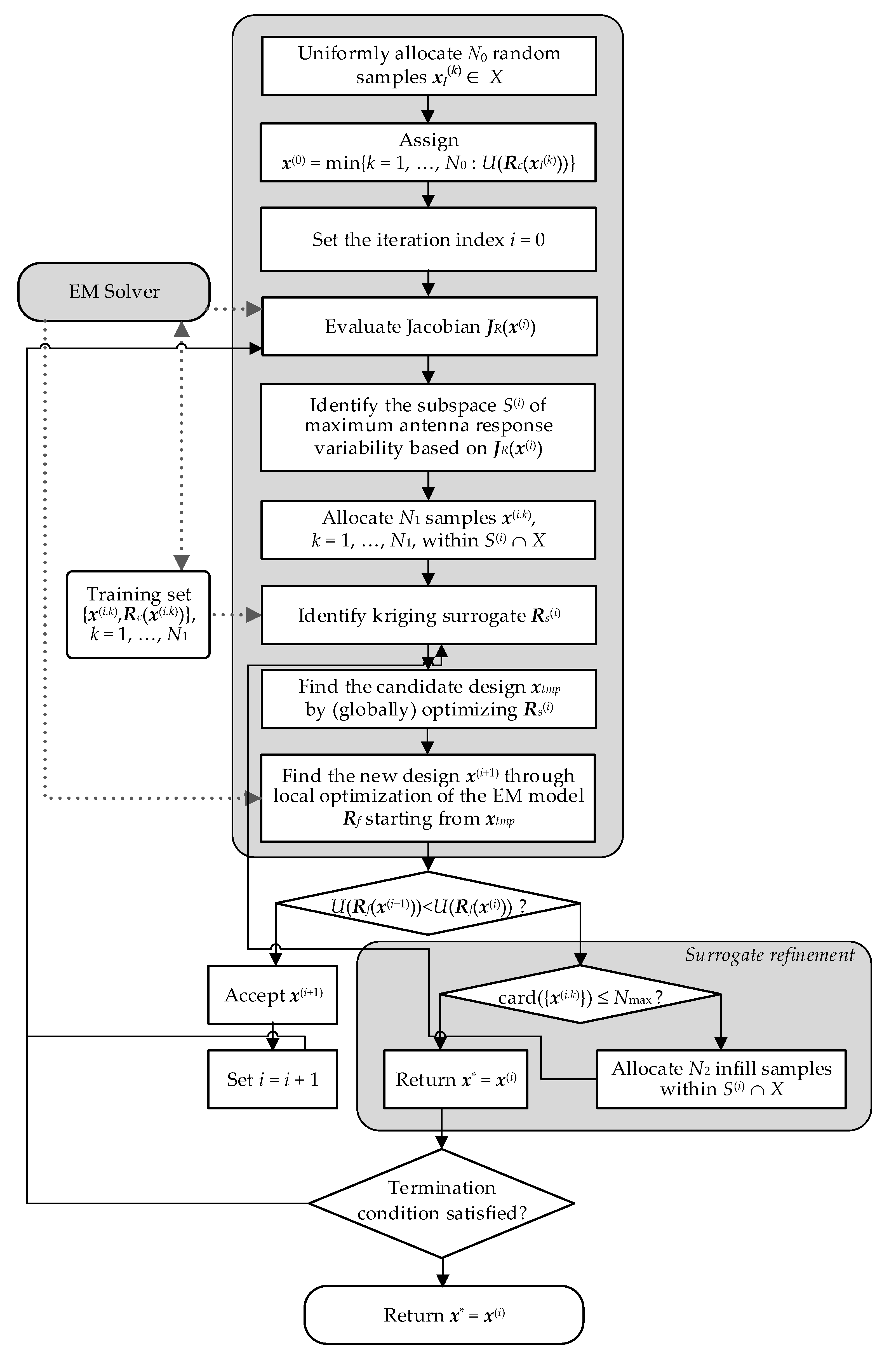
Algorithm 1 PCA-based optimization algorithm using variable-fidelity EM simulations
1.	Initial sampling: Uniformly allocate N0 random samples xI(k) ϵ X;
2.	Identify the best design x(0) = min{k = 1, …, N0: U(Rc(xI(k)))};
3.	Set the iteration index i = 0;
4.	Evaluate the high-fidelity response Rf(x(i)) and the corresponding Jacobian JR(x(i));
5.	Use JR(x(i)) to identify the subspace S(i) of maximum antenna response variability (Section 2.3);
6.	Allocate N1 samples x(i.k), k = 1, …, N1, within S(i) ∩ X;
7.	Identify the kriging surrogate Rs(i) therein using {x(i.k),Rc(x(i.k))} as the training set (Section 2.4);
8.	Find the candidate design xtmp by (globally) optimizing the surrogate Rs(i) [37]: $$x_{tmp}=\arg \underset{x\in S^{(i)}\cap X}{\min }U(R_s^{(i)}(x))$$ (10)
9.	Starting from xtmp, find the new design x(i+1) through local optimization of the EM model Rf (cf. Section 2.5) [37] $$x^{(i+1)}=\arg \underset{x\in X}{\min }U(R_f(x))$$ (11)
10.	ifU(Rf(x(i+1))) < U(Rf(x(i))) then
11.	Accept x(i+1) and set i = i + 1;
12.	else
13.	if card({x(i.k)}) ≤ Nmax then
14.	Allocate N2 additional (infill) samples within S(i) ∩ X; go to 7;
15.	else
16.	Return x* = x(i).
17.	end
18.	end
19.	If the termination condition is not satisfied, go to 4; else return x* = x(i).

The Algorithm 1 is initialized by rough exploration of the parameter space and executing the main algorithm starting from the best point x⁽⁰⁾ found at that stage of the process. In each iteration, the affine subspace S⁽ⁱ⁾ is defined using the principal components of the Jacobian matrix (evaluated at the level of the high-fidelity EM model). As mentioned before, the principal components correspond to the directions of the maximum antenna response variability (Steps 4 and 5). Because S⁽ⁱ⁾ is low dimensional (typically, only two eigenvectors are employed), it is possible to construct a reliable surrogate within S⁽ⁱ⁾ ∩ X using a small number of samples N₁ (Steps 6 and 7). The primary role of the surrogate is to determine the globally best design on S⁽ⁱ⁾ ∩ X (Step 8). Note that the above exploration stage is conducted at the level of the low-fidelity model. The next step is an expedited local optimization of the high-fidelity EM model (Step 9). This concludes an iteration of the procedure, which is then repeated until convergence or until the computational budget assigned for the procedure is exceeded. In the case of failure of an iteration, i.e., inability of finding a better design, the surrogate model is refined by adding infill samples (Step 10). Figure 2 provides a graphical illustration of the essential Algorithm 1 stages. Note that Steps 1 and 2 can be replaced by employing a user-supplied initial design. The overall flowchart of the Algorithm 1 can be found in Figure 3.

3. Results

In this section, the proposed design optimization methodology is validated using two examples of microstrip antennas, a wideband monopole and a uniplanar triple-band dipole. To verify the quasi-global optimization capabilities, our algorithm is compared to multiple-start gradient search. For meaningful performance determination, benchmarking is carried out based on the result statistics obtained for twenty independent algorithm runs. Furthermore, to corroborate the benefits of employing variable-fidelity simulations, the comparative studies also include an algorithm version involving only the high-fidelity model.

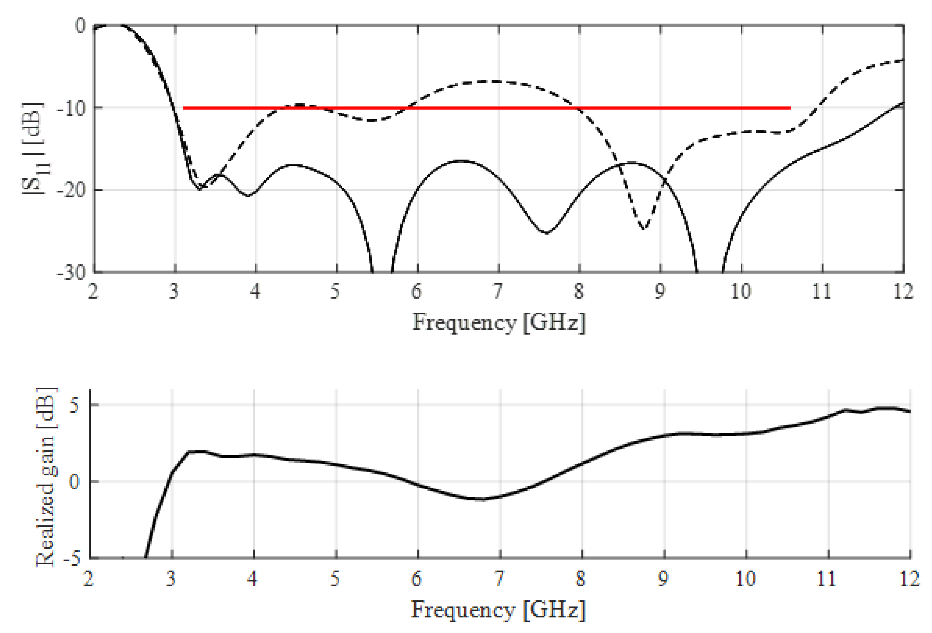
3.1. Example I: Wideband Monopole Antenna

Our first verification case is an ultra-wideband monopole antenna with quasi-circular radiator and a modified ground plane for bandwidth enhancement [39]. The antenna geometry is shown in Figure 4a. The design variables are x = [L₀ dR R r_rel dL dw L_g L₁ R₁ dr c_rel]^T. The structure is implemented on Rogers RO4350 substrate (ε_r = 3.5, tanδ = 0.0027, h = 0.76 mm). The computational models are implemented in CST Microwave Studio and evaluated using its time-domain solver:

• High-fidelity model R_f: 1.588.000 mesh cells, simulation time 362.6 s;
• Low-fidelity model R_c1: 323.000 mesh cells, simulation time 66.9 s;
• Low-fidelity model R_c2: 185.000 mesh cells, simulation time 51.3 s.

The two versions of the low-fidelity models are used to run the algorithm independently for the following combinations: R_c1-R_f and R_c2-R_f (as low- and high-fidelity models, respectively). The model R_c1 is set at the discretization density normally used by variable-fidelity procedures, i.e., with retaining good correlations with the high-fidelity version. The second model is much coarser and normally of insufficient quality to be employed in the procedures such as space mapping [40]. The reason for considering these two versions is to verify whether the application of the overly coarse model at the exploratory stages of the optimization process is sufficient to ensure the overall reliability of the algorithm.

The parameter space X for the problem is defined by the lower bounds l = [4.0 0.0 3.0 0.1 0.0 0.0 4.0 0.0 2.0 0.2 0.2]^T and the upper bounds u = [15.0 6.0 8.0 0.9 5.0 8.0 15.0 6.0 5.0 1.0 0.9]^T. The steps for estimating the Jacobian through the finite differentiation are d = [0.1 0.1 0.1 0.02 0.1 0.1 0.1 0.1 0.1 0.02 0.1]^T. The design objective is to minimize |S₁₁| within the UWB frequency range of 3.1 GHz to 10.6 GHz.

The experimental setup adheres to the following rules:

• A total of 20 runs of the proposed algorithm are executed using new set of samples x_I^(k) for each run. The computational budget set to 300 (equivalent) high-fidelity EM simulations of the antenna. The cost is calculated as N_f + N_c/T where N_f and N_c are the numbers of high- and low-fidelity model evaluations, whereas T is the time evaluation ratio between the high- and low-fidelity models;
• (Benchmark) 20 runs of local search using the trust-region algorithm with numerical derivatives are executed with random initial points employed at each run;
• (Benchmark) 20 runs of the proposed globalized search are executed with high-fidelity model used at both the exploratory and local tuning stages.

The specific setup of the control parameters (the same for this and the next test problem) was the following: N₀ = 50 (initial number of training data samples for surrogate model construction), N₁ = 30 (the number of infill samples assigned using sequential sampling, cf. Section 2.4), N₂ = 20 (the maximum number of additional samples, Step 10 of the algorithm), which gives N_max = 100 (the maximum overall budged for surrogate model construction). The dimensionality of the subspace for surrogate model construction was two. The latter was chosen to ensure a construction of reliable surrogate using relatively small number of data samples but also the fact that the eigenvalues of the covariance matrix C are quickly descending (i.e., only a few principal directions really matter).

The result statistics are shown in

Table 1. Optimization results for wideband monopole antenna.

Algorithm	Cost			Success Rate ##	max|S11| $	std max|S11| *
	Number of High-Fidelity Evaluations Nf	Number of Low-Fidelity Evaluations Nc	Total Cost #
Multiple-start gradient search	90.4	N/A	90.4	0.4	–6.6 dB	5.9 dB
Quasi-global search (Rf only)	287.1	N/A	287.1	1.0	–14.5 dB	1.5 dB
Quasi-global search (Rc1 + Rf) [This work]	95.2	247.0	140.7	1.0	–14.4 dB	0.8 dB
Quasi-global search (Rc2 + Rf) [This work]	93.1	266.6	135.4	1.0	–14.6 dB	0.94 dB

# EM simulation count averaged over twenty algorithm runs with random initial points. The cost is calculated at N_f + N_c/T where T is the time evaluation ratio between the high- and low-fidelity model. ## Proportion of runs where maximum |S₁₁| within frequency range was at least –10dB. $ Maximum |S₁₁| within frequency range averaged over twenty runs. * Standard deviation of max in-band gain in dB across the set of twenty algorithm runs.

. Note that the algorithm presented in this work yields satisfactory results (i.e., with the maximum in-band reflection below –10 dB) in all runs. At the same time, the benchmark algorithm (multiple-start gradient search) only exhibits about forty percent success rate. The computational cost of our methodology is very low, especially for the version working with the coarser low-fidelity model R_c2. It should be noted that involving variable-fidelity models does not lead to a reliability degradation which can be observed by comparison with the algorithm version using high-fidelity model at all stages of the optimization process. Figure 5 shows the antenna reflection responses at the design x⁽⁰⁾ (cf. Step 2, Section 2.6) and upon optimization for a selected algorithm run, along with the realized gain at the optimum design.

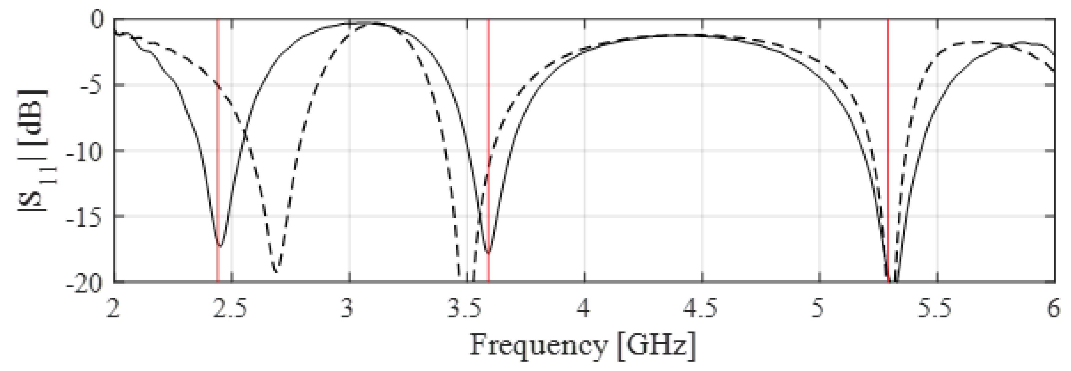
3.2. Example II: Triple-Band Uniplanar Dipole Antenna

The second verification case is a triple-band uniplanar dipole antenna shown in Figure 4b. The structure is based on the design of [41], implemented on RO4350 substrate, and fed through a 50-ohm coplanar waveguide (CPW). The design variables are x = [l₁ l₂ l₃ l₄ l₅ w₁ w₂ w₃ w₄ w₅]^T. Other parameters are fixed: l₀ = 30, w₀ = 3, s₀ = 0.15 and o = 5 (all dimensions in mm). The computational models are implemented in CST Microwave Studio and evaluated using its time-domain solver:

• High-fidelity model R_f:: 185.000 mesh cells, simulation time 222.1 s;
• Low-fidelity model R_c1: 70.000 mesh cells, simulation time 51.0 s;
• Low-fidelity model R_c2: 40.000 mesh cells, simulation time 32.0 s.

The parameter space X is defined by l = [35 10 25 10 18 0.5 0.5 0.5 0.5 0.5]^T and u = [40 15 30 15 22 2 1 1 1 1]^T. The steps for estimating the Jacobian through the finite differentiation are d = [0.1 0.1 0.1 0.1 0.1 0.05 0.05 0.05 0.05 0.05]^T. The design objective is to minimize |S₁₁| within the following bands: 2.4 GHz to 2.5 GHz, 3.55 GHz to 3.65 GHz, and 5.25 GHz to 5.35 GHz.

The experimental setup is the same as for the first test case.

Table 2. Optimization results for triple-band dipole antenna.

Algorithm	Cost			Success Rate ##	max|S11| $	std max|S11| *
	Number of High-Fidelity Evaluations Nf	Number of Low-Fidelity Evaluations Nc	Total Cost #
Multiple-start gradient search	99.4	N/A	99.4	0.25	–5.68 dB	4.9 dB
Quasi-global search (Rf only)	274.81	N/A	274.1	0.95	–13.5 dB	1.2 dB
Quasi-global search (Rc1 + Rf) [This work]	100.3	200.4	147.3	1.0	–13.5 dB	0.5 dB
Quasi-global search (Rc2 + Rf) [This work]	99.7	209.7	129.4	1.0	–13.5 dB	0.5 dB

# EM simulation count averaged over twenty algorithm runs with random initial points. The cost is calculated at N_f + N_c/T where T is the time evaluation ratio between the high- and low-fidelity model. ## Proportion of runs where maximum |S₁₁| within frequency range was at least –10dB. $ Maximum |S₁₁| within frequency range averaged over twenty runs. * Standard deviation of max in-band gain in dB across the set of twenty algorithm runs.

gathers the numerical results. Overall, the performance of the proposed algorithm is consistent with what was observed for the first verification case. In particular, satisfactory designs, i.e., ensuring appropriate allocation of the antenna resonances, are found in almost all algorithm runs. At the same time, the success rate for the benchmark algorithm is only about twenty five percent. This confirms that need for global search. The reflection responses at x⁽⁰⁾ and at the optimized design for a selected algorithm run are shown in Figure 6.

3.3. Discussion

The results presented in Section 3.1 and Section 3.2 permit the following conclusions concerning the presented quasi-global optimization procedure:

• Our approach significantly improves the reliability of the optimization process compared to multiple-start local routines;
• The computational cost of the algorithm is very low (about 140 equivalent high-fidelity EM model evaluation on the average), especially when taking into account its global search capabilities;
• Repeatability of results is excellent, which is demonstrated by low values of the standard deviation of the final objective function values;
• Robustness of the method is retained even if the algorithm is executed with a coarser version of the low-fidelity model. Clearly, a reduced performance sensitivity to the low-fidelity model setup is a practically attractive feature. This is a consequence of separating the exploratory and local tuning stages of the process;
• For the same reason, the quality of the designs rendered by the proposed procedure is similar to that produced by the algorithm merely using the high-fidelity model; in comparison to that version, the CPU cost is reduced by a factor of two.

Given the above properties, the proposed method can be considered a viable and low-cost alternative to population-based metaheuristics, currently being the most widely used solution approaches to global optimization tasks.

4. Conclusions

In the paper, a novel procedure for globalized design optimization of antenna structures has been proposed. The methodology combines surrogate-assisted exploration of the parameter space as well as expedited trust-region gradient-based local refinement. To ensure low cost of the parameter tuning process, the exploration step is carried out over the low-dimensional affine subspaces spanned by the principal components of the antenna response gradients, which determine the directions of the maximum variability of antenna characteristics, averaged of the frequency range of interest. Further improvement of the computational efficiency is achieved by incorporating variable-fidelity simulation models. Our technique has been comprehensively validated using two examples of microstrip antennas, a wideband monopole and a triple-band uniplanar dipole. The statistics computed from multiple algorithm runs demonstrate reliability of the optimization process and superior result repeatability with satisfactory designs found in almost all algorithm executions. The efficacy of multiple-start local search employed as benchmark is significantly worse with only forty and twenty-five percent of success rate for the considered test cases, respectively. At the same time, the employment of variable-fidelity simulations enables further computational savings as compared to the algorithm using only the high-fidelity model. Our comparative studies indicate that the procedure delivers quality results even if the underlying low-fidelity model is much coarser than what would normally be required by variable-fidelity procedures (e.g., space mapping), which is achieved by a separation of the exploratory and local tuning steps of the process. Quasi-global search capability, straightforward implementation, and remarkably low CPU cost being a small fraction of expenses entailed by population-based metaheuristics are the major advantages of the presented methodology. All of these can make it an attractive alternative to the existing methodologies.

References

1. Su, S.; Lee, C.; Hsiao, Y. Compact two-inverted-F-antenna system with highly integrated π-shaped decoupling structure. IEEE Trans. Ant. Propag. 2019, 67, 6182–6186. [Google Scholar] [CrossRef]
2. Yazeen, P.S.M.; Vinisha, C.V.; Vandana, S.; Suprava, M.; Nair, R.U. Electromagnetic Performance Analysis of Graded Dielectric Inhomogeneous Streamlined Airborne Radome. IEEE Trans. Antennas Propag. 2017, 65, 1. [Google Scholar] [CrossRef]
3. Ta, S.X.; Choo, H.; Park, I. Broadband Printed-Dipole Antenna and Its Arrays for 5G Applications. IEEE Antennas Wirel. Propag. Lett. 2017, 16, 2183–2186. [Google Scholar] [CrossRef]
4. Pietrenko-Dabrowska, A.; Koziel, S. Computationally-efficient design optimisation of antennas by accelerated gradient search with sensitivity and design change monitoring. IET Microw. Antennas Propag. 2020, 14, 165–170. [Google Scholar] [CrossRef]
5. Gregory, M.D.; Bayraktar, Z.; Werner, D.H. Fast Optimization of Electromagnetic Design Problems Using the Covariance Matrix Adaptation Evolutionary Strategy. IEEE Trans. Antennas Propag. 2011, 59, 1275–1285. [Google Scholar] [CrossRef]
6. Bhattacharya, R.; Garg, R.; Bhattacharyya, T.K. Design of a PIFA-Driven Compact Yagi-Type Pattern Diversity Antenna for Handheld Devices. IEEE Antennas Wirel. Propag. Lett. 2015, 15, 1. [Google Scholar] [CrossRef]
7. Rahman, M.; Naghshvarianjahromi, M.; Mirjavadi, S.S.; Hamouda, A. Compact UWB Band-Notched Antenna with Integrated Bluetooth for Personal Wireless Communication and UWB Applications. Electronics 2019, 8, 158. [Google Scholar] [CrossRef] [Green Version]
8. Rahman, M.; Naghshvarianjahromi, M.; Mirjavadi, S.S.; Hamouda, A. Bandwidth Enhancement and Frequency Scanning Array Antenna Using Novel UWB Filter Integration Technique for OFDM UWB Radar Applications in Wireless Vital Signs Monitoring. Sensors 2018, 18, 3155. [Google Scholar] [CrossRef] [Green Version]
9. Rahman, M.; Naghshvarianjahromi, M.; Mirjavadi, S.S.; Hamouda, A. Resonator Based Switching Technique between Ultra Wide Band (UWB) and Single/Dual Continuously Tunable-Notch Behaviors in UWB Radar for Wireless Vital Signs Monitoring. Sensors 2018, 18, 3330. [Google Scholar] [CrossRef] [Green Version]
10. Palacios, J.; De Donno, D.; Widmer, J. Lightweight and Effective Sector Beam Pattern Synthesis With Uniform Linear Antenna Arrays. IEEE Antennas Wirel. Propag. Lett. 2016, 16, 605–608. [Google Scholar] [CrossRef]
11. Ehrenborg, C.; Gustafsson, M. Fundamental Bounds on MIMO Antennas. IEEE Antennas Wirel. Propag. Lett. 2017, 17, 21–24. [Google Scholar] [CrossRef] [Green Version]
12. Akyol, S.; Alatas, B. Plant intelligence based metaheuristic optimization algorithms. Artif. Intell. Rev. 2016, 47, 417–462. [Google Scholar] [CrossRef]
13. Jian, R.; Chen, Y.; Chen, T. Multi-Parameters Unified-Optimization for Millimeter Wave Microstrip Antenna Based on ICACO. IEEE Access 2019, 7, 53012–53017. [Google Scholar] [CrossRef]
14. Smith, J.; Baginski, M.E. Thin-Wire Antenna Design Using a Novel Branching Scheme and Genetic Algorithm Optimization. IEEE Trans. Antennas Propag. 2019, 67, 2934–2941. [Google Scholar] [CrossRef]
15. Lalbakhsh, A.; Afzal, M.U.; Esselle, K.P. Multi-objective Particle Swarm Optimization to Design a Time Delay Equalizer Metasurface for an Electromagnetic Band Gap Resonator Antenna. IEEE Antennas Wirel. Propag. Lett. 2016, 16, 1. [Google Scholar] [CrossRef]
16. Goudos, S.K. Antenna Design Using Binary Differential Evolution: Application to discrete-valued design problems. IEEE Antennas Propag. Mag. 2017, 59, 74–93. [Google Scholar] [CrossRef]
17. Baumgartner, P.; Bauernfeind, T.; Biro, O.; Hackl, A.; Magele, C.; Renhart, W.; Torchio, R. Multi-Objective Optimization of Yagi–Uda Antenna Applying Enhanced Firefly Algorithm With Adaptive Cost Function. IEEE Trans. Magn. 2018, 54, 1–4. [Google Scholar] [CrossRef]
18. Subhashini, K.R. Antenna array synthesis using a newly evolved optimization approach: Strawberry algorithm. J. Electr. Eng. 2019, 70, 317–322. [Google Scholar] [CrossRef] [Green Version]
19. Wang, G.-G.; Deb, S.; Cui, Z. Monarch butterfly optimization. Neural Comput. Appl. 2015, 31, 1995–2014. [Google Scholar] [CrossRef] [Green Version]
20. Salgotra, R.; Singh, U. A novel bat flower pollination algorithm for synthesis of linear antenna arrays. Neural Comput. Appl. 2016, 30, 2269–2282. [Google Scholar] [CrossRef]
21. Alzahed, A.; Mikki, S.; Antar, Y.M. Nonlinear Mutual Coupling Compensation Operator Design Using a Novel Electromagnetic Machine Learning Paradigm. IEEE Antennas Wirel. Propag. Lett. 2019, 18, 861–865. [Google Scholar] [CrossRef]
22. Tak, J.; Kantemur, A.; Sharma, Y.; Xin, H. A 3-D-Printed W-Band Slotted Waveguide Array Antenna Optimized Using Machine Learning. IEEE Antennas Wirel. Propag. Lett. 2018, 17, 2008–2012. [Google Scholar] [CrossRef]
23. Bin Liu, J.; Shen, Z.X.; Lu, Y.L. Optimal Antenna Design With QPSO–QN Optimization Strategy. IEEE Trans. Magn. 2014, 50, 645–648. [Google Scholar] [CrossRef]
24. Pantoja, M.F.; Meincke, P.; Bretones, A.C.R. A Hybrid Genetic-Algorithm Space-Mapping Tool for the Optimization of Antennas. IEEE Trans. Antennas Propag. 2007, 55, 777–781. [Google Scholar] [CrossRef]
25. Zaharis, Z.; Lazaridis, P.; Cosmas, J.; Skeberis, C.; Xenos, T.D. Synthesis of a Near-Optimal High-Gain Antenna Array With Main Lobe Tilting and Null Filling Using Taguchi Initialized Invasive Weed Optimization. IEEE Trans. Broadcast. 2014, 60, 120–127. [Google Scholar] [CrossRef] [Green Version]
26. Koziel, S.; Bekasiewicz, A. Multi-Objective Design of Antennas Using Surrogate Models; World Scientific Pub Co Pte Lt: Singapore, 2016. [Google Scholar]
27. Koziel, S.; Leifsson, L. (Eds.) Surrogate-based modeling and optimization. In Applications in Engineering; Springer: New York, NY, USA, 2013. [Google Scholar]
28. Hao, Z.-C.; He, M.; Hong, W. Design of a Millimeter-Wave High Angle Selectivity Shaped-Beam Conformal Array Antenna Using Hybrid Genetic/Space Mapping Method. IEEE Antennas Wirel. Propag. Lett. 2015, 15, 1208–1212. [Google Scholar] [CrossRef]
29. Koziel, S.; Unnsteinsson, S.D. Expedited Design Closure of Antennas by Means of Trust-Region-Based Adaptive Response Scaling. IEEE Antennas Wirel. Propag. Lett. 2018, 17, 1099–1103. [Google Scholar] [CrossRef]
30. Koziel, S.; Bekasiewicz, A. Expedited simulation-driven design optimization of UWB antennas by means of response features. Int. J. RF Microw. Comput. Eng. 2017, 27, e21102. [Google Scholar] [CrossRef]
31. Koziel, S.; Pietrenko-Dabrowska, A. Performance-Driven Surrogate Modeling of High-Frequency Structures; Springer Science and Business Media LLC: Berlin/Heidelberg, Germany, 2020. [Google Scholar]
32. Richards, L.E.; Jolliffe, I.T. Principal Component Analysis. J. Mark. Res. 1988, 25, 410. [Google Scholar] [CrossRef]
33. Kleijnen, J.P.C. Kriging metamodeling in simulation: A review. Eur. J. Oper. Res. 2009, 192, 707–716. [Google Scholar] [CrossRef] [Green Version]
34. Ai, M.; Kong, X.; Li, K. A general theory for orthogonal array based Latin hyper-cube sampling. Stat. Sin. 2016, 26, 761–777. [Google Scholar]
35. Forrester, A.I.J.; Keane, A. Recent advances in surrogate-based optimization. Prog. Aerosp. Sci. 2009, 45, 50–79. [Google Scholar] [CrossRef]
36. Couckuyt, I. Forward and inverse surrogate modeling of computationally expen-sive problems. PhD Thesis, Ghent University, Gent, Belgium, 2013. [Google Scholar]
37. Conn, A.R.; Gould, N.I.M.; Toint, P.L. Trust region methods; Society for Industrial and Applied Mathematics: Philadelphia, PA, USA, 2000. [Google Scholar]
38. Broyden, C.G. A class of methods for solving nonlinear simultaneous equations. Math. Comp. 1965, 19, 577–593. [Google Scholar] [CrossRef]
39. Alsath, M.G.N.; Kanagasabai, M.; Alsath, M.G.N. Compact UWB Monopole Antenna for Automotive Communications. IEEE Trans. Antennas Propag. 2015, 63, 1. [Google Scholar] [CrossRef]
40. Zhu, J.; Bandler, J.W.; Nikolova, N.K.; Koziel, S. Antenna Optimization through Space Mapping. IEEE Trans. Antennas Propag. 2007, 55, 651–658. [Google Scholar] [CrossRef] [Green Version]
41. Chen, Y.-C.; Chen, S.-Y.; Hsu, P. Dual-Band Slot Dipole Antenna Fed by a Coplanar Waveguide. In Proceedings of the 2006 IEEE Antennas and Propagation Society International Symposium, Albuquerque, NM, USA, 9–14 July 2006; pp. 3589–3592. [Google Scholar] [CrossRef]
Figure 1. Exemplary reflection responses of (a) wideband monopole and (b) uniplanar triple-band dipole antenna at random designs: high-fidelity model (— blue), (finer) low-fidelity model (- - - black), (coarser) low-fidelity model (⋅⋅⋅⋅ green). Note that the finer version of the low-fidelity model retains good correlation with the high-fidelity one, but the correlation is not as good for the coarser version. Thus, the coarser low-fidelity model is insufficient for local search purposes (e.g., within space mapping or feature-based optimization frameworks), yet it might be still applicable for global design space exploration.
Electronics 09 00673 g001
Figure 2. Basic steps of the proposed quasi-global optimization procedure (illustrated for a three-dimensional case): (a) parameter space X, initial sampling, and the best design x(0) over the sample set (Steps 1 and 2), (b) first iteration: subspace S(0) spanned by the first two principal directions (Steps 4 and 5), (c) sampling of S(0) ∩ X (Step 6), construction of the surrogate (Step 7), subsequently optimized to find xtmp (Step 8), and the follow-up gradient-based refinement yielding the next design x(1) (Step 9).
Electronics 09 00673 g002
Figure 3. Flowchart of the proposed globalized design optimization procedure (Algorithm 1).
Electronics 09 00673 g003
Figure 4. Verification case studies: (a) ultra-wideband monopole [39] (ground plane shown using light-shade gray), and (b) triple-band uniplanar dipole [41].
Electronics 09 00673 g004
Figure 5. Ultra-wideband monopole antenna: reflection responses at x(0) (- - -) and at the optimized design (—) for the selected run of the proposed algorithm. The horizontal line indicates design specifications, i.e., –10 dB acceptance level for antenna reflection within 3.1 GHz to 10.6 GHz frequency range. The bottom plot illustrates realized gain at the optimum design.
Electronics 09 00673 g005
Figure 6. Triple-band uniplanar dipole antenna: reflection responses at x(0) (- - -) and at the optimized design (—) for the selected run of the proposed algorithm. The vertical lines indicate the target operating frequencies.
Electronics 09 00673 g006