Effective Position Control for a Three-Phase Motor
by
 , , , and
Patxi Alkorta
1,* ,
,
Oscar Barambones
2,
José Antonio Cortajarena
1,
Itziar Martija
3 and
Fco. Javier Maseda
3 1
Engineering School of Gipuzkoa, University of the Basque Country; Otaola hirib. 29, 20600 Eibar, Spain
2
Engineering School of Vitoria, University of the Basque Country; Nieves Cano 12, 01006 Vitoria, Spain
3
Engineering School of Bilbao, University of the Basque Country; Rafael Moreno 3, 48013 Bilbao, Spain
*
Author to whom correspondence should be addressed.
Electronics 2020, 9(2), 241; https://doi.org/10.3390/electronics9020241
Submission received: 31 December 2019
/
Revised: 24 January 2020
/
Accepted: 27 January 2020
/
Published: 1 February 2020
(This article belongs to the Special Issue Advanced Control Systems for Electric Drives)
Abstract
:This document presents an efficient proportional derivative (PD) position controller for three-phase motor drives. The regulator has been designed in frequency domain, employing the direct–quadrature (d–q) synchronous rotating reference frame and the indirect vector control. The presented position regulator is easy to tune and incorporates a feed forward (FF) term to compensate effectively the effect of the load disturbance. This position controller has been validated experimentally by using two industrial three-phase motors: an induction motor (IM) of 7.5 kW and a permanent magnet synchronous motor (PMSM) of 3.83 kW. The inner proportional integral (PI) current loops of both machines have also been designed in the frequency domain. Each machine has connected in its shaft an incremental encoder of 4096 pulses per revolution, to measure the position. Several simulations and experimental tests have been carried out with both motors, in favorable conditions and also with various types of adversities (parametric uncertainties, unknown load disturbance and measurement noise in the position and current loops), getting very good results and suggesting that this controller could be used in the research area and also in the industry.
1. Introduction
Three-phase motors are widely used in civil engineering and in industry applications, where the most employed are the induction motor (IM) and permanent magnet synchronous motor (PMSM). IM are the most used machines in general (cranes, heavy industrial processes, motor pumps, trains, etc.), but the use of permanent magnet synchronous motors are increasing considerably last years (tool machines, electrical vehicles, etc.). IM offers good characteristics like a low maintenance, low moment of inertia, robust architecture, low torque ripple and low price. On the other hand, PMSM provides very good torque–weight ratio, high efficiency and accuracy. Depending on the application, both kinds of motors are controlled by using the Direct Torque Control (DTC) or Field Oriented Control (FOC) techniques. The FOC or vector control strategy is well settled such in civil engineering as in the industry, due to the fact that this technique gets excellent dynamics performance of the three-phase machine. That is due to using FOC techniques the three-phase machine is controlled like an independent excitation Direct Current (DC) machine, in which the electromagnetic torque and field flux are controlled separately [1]. This way, in the three-phase machine are also controlled independently the electromagnetic torque and rotor flux. The position control of the three-phase motor is an application that takes advantage the vector control benefits. One of the first research works related is [2], in which the experimental implementation by using FOC for speed and position control of IM and PMSM is presented. Very interesting position control schemes for IM are presented during the last decades, by using the classical proportional derivative (PD)/PID [3,4], and by employing advanced position regulators as a fuzzy [5], passivity-based [6], model predictive control [7], sliding-mode control [8,9], optimization-based sensorless [10] and poles placement [11]. Regarding PMSM, it is typical to find sensorless-based research works due to that position sensorless techniques are considerably easier to implement in these machines than in induction ones, where the classical PD/PID algorithms are employed in the position regulation loops [12,13]. However, to get high accuracy is necessary to have installed the position sensor in the system. Thus, several advanced position controllers as a sliding-mode control [14,15], fuzzy [16,17,18] and model predictive control [19,20] are presented. All these position controllers provide good dynamics and high accuracy, in spite of much of them not detailing the last one explicitly. Taking similar conditions in experiments, for IM [8] offers best steady-steady state accuracy, getting between 0 and 0.00038 rad of the position error, [7] and [11] provide an accuracy of 0.005 rad, while the steady-steady state accuracy of the presented proposal for IM is very close to it, 0.007 rad. On the other hand, for PMSM, [14] offers a position accuracy between 0.002 and 0.005 rad, [17] provides a position accuracy around 0.017 rad, while the presented proposal provides an accuracy of 0.002 rad. This way, advanced controllers provide excellent performance to these machines, but their control laws and tuning can be too complex to use them experimentally, i.e., in the industry, much of them do not offer a clear way or rules to tune. The real applications area needs efficient controllers but at the same time be easy to tune. The presented position regulator provides good dynamics and high accuracy, it is easy to tune with a simple control law and it is valid for different three-phase motors. In [4], a PD position controller tuned in the frequency domain for IM was presented and experimentally validated. The presented proposal in this paper takes this PD regulator and extends to the PMSM the experimental validation. Moreover, practical tuning recommendations for both motors are given and experimental comparatives between them are done.
The goal of this paper is to offer an effective and easy to tune PD position controller for the most employed three-phase machines, that is IM and PMSM. The paper is organized as follows. Section 2 describes the dynamics of the motors and the position and current regulators design in the frequency domain with the study of stability. Section 3 presents the employed two tests benches, and the tests (simulations and real experiments) done with both motors. Finally, Section 4 discusses and gets the conclusions.
2. Three-Phase Motor Position Proportional Derivative Controller Design
2.1. Induction Motor Dynamics
Induction motor dynamics can be expressed by employing the next five differential equations, expressed in the direct–quadrature (d–q) synchronous rotating reference frame and taking that the q (quadrature) component of the stator current (electromagnetic torque current component, isq) and the d (direct) component of the stator current (rotor flux current component, isd) are decoupled, due to that the q component of rotor flux is null, ψrq = 0 and this way the rotor flux is the same as its d (direct) component, ψr = ψrd, [21],
where TL is the load disturbance, ϴm is the mechanical position, ωs is the synchronous speed, vsd is the d component of the stator voltage and vsq is the q component of the stator voltage. The rest of the parameters are described in Section 3.1.1. As it is well known, the isd current is employed to regulate the ψr rotor flux of the machine. This flux keeps constant its value, the typically rated value. Then, considering the steady state and taking Equation (3), it is possible to get the relation between both variables,
and taking Equation (2) of the electromagnetic torque, it can be expressed as
where the KT torque constant is defined as
Now Equation (7) can be replaced in Equation (1), obtaining the following Expression (9), which contains the first three equations.
This way, Equation (9) contains the electromagnetic and mechanical equations, while Equations (4) and (5) contain the electrical equations.
2.2. Permanent Magnet Synchronous Motor Dynamics
PMSM motor dynamics are shown by using the next four differential equations, where like in the previous case (IM), all of them are expressed in a d–q synchronous rotating reference frame and supposing that the isq electromagnetic torque current component and the isd rotor flux current component are decoupled, that is ψrq = 0 and ψr = ψrd. Moreover, as the PMSM has its own rotor flux generated by its rotor magnets, that is ψM (constant), then rotor flux generated electrically is usually fixed to zero, and consequently isd = 0, [22],
where ωr is the electrical rotor speed, and the rest of the parameters are described in Section 3.1.2. As the ψM is constant, then Equation (11) of the electromagnetic torque can be rewritten as follows,
where the KT torque constant is,
As in the IM case, Equation (14) can be replaced in Equation (10), obtaining the following Expression (17), which contains the first two equations of the dynamics of PMSM,
In this sense, Equation (16) contains the electromagnetic and mechanical equations, while Equations (12) and (13) contain the electrical equations.
2.3. Position Proportional Derivative with a Feed-Forward Controller Design
Figure 1 shows the complete vector position control scheme for the three-phase motor scheme, employing the d–q synchronous rotating reference frame. The objective of this scheme is to regulate the ϴm mechanical position of the motor’s shaft, which is the main variable (outer loop), by using the PDϴm regulator. This regulator provides the best electromagnetic torque current reference, isq*, according to (7) and (15). On the other hand, the rotor flux current reference, isd*, imposes the value of the rotor flux that the motor needs. This way, the inner loops (current loops) are controlled by two PI regulators, where their objective is to get the best voltage references, vsd* and vsq*, corresponding to their current references, isd* and isq*, respectively. The ABC -> dq block implements the Clarke–Park transformations, and the dq -> ABC block the inverse Park–Clarke transformations. The voltage sourced inverter (VSI) block represents the three-phase Voltage Sourced Inverter, which receives the control signals from the SVPWM (Space Vector Pulse Width Modulation) block. This modulator generates the control signals according to the voltage references obtained from the inner loops, asking to the inverter to generate these voltages in its three-phase output. Calc ϴs calculates the d–q synchronous rotating reference frame’s angle with respect the α–β stationary reference frame. For that it is used the indirect vector control, by integrating the ωs synchronous speed. Thus for the PMSM motor, this speed is the same as the ωr electrical speed
which is obtained from the ωm mechanical speed (measured) by using this expression,
On the other hand, for the IM motor, this speed is given by Equation (19),
where the ωslip slip speed is calculated easily with Equation (20)
As we have seen in the previous subsections, both three-phase machines have the same electromechanical Equations (9) and (16). This way, the design of the position regulator for both is the same. Taking into account that the dynamics of the two PI current regulators, the SVPWM modulator and the VSI inverter are faster than the electromechanical and PD dynamics, then the following simplified scheme can be obtained,
Thus, taking the electromechanical equation and considering null the load disturbance (TL = 0) and applying Laplace’s transformation, the following transfer function can be obtained
where τm = J/Bv is the mechanical time constant. Now taking the causal PD regulator
where Kpϴm and Kdϴm are the proportional and derivative coefficients, respectively, of the PD regulator, and val is the absolute value of the pole to convert this regulator in the causal transfer function. This value has to be large enough to simplify its dynamics compared with the zero’s dynamics.
The open loop transfer function (OLTF) of the simplified diagram presented in Figure 2, can be obtained as:
It is well known from engineering control that at the ωGCϴm gain cross-over frequency the module is the unity
and the phase Equation is (26), where PMϴm is the phase margin of the position loop
Now, taking the system of these two Equations, (25) and (26), where the ωGCϴm and PMϴm are the design data, and by solving them, the two coefficients of the PD regulator (Kpϴm and Kdϴm) necessary for that will be obtained. For this resolution, the following group of intermediate variables are necessary (den,a,b)
The effect of the TL load disturbance can produce important problems when the objective is to get an efficient position tracking. To avoid this problem, it can be added as a Feed-Forward (FF) action in the controller, where for that it is necessary to know the disturbance’s value, Figure 3. This way, the control law contains both actions, PD and FF,
As in many cases it is impossible to know the load disturbance, and therefore an easy way to solve this issue is to estimate it by using a load estimator or observer. A simple and effective load observer is obtained directly from the electromechanical Equation (9)/(16),
2.4. Current Proportional Integral Controllers Design
The design of the current regulators or inner loops for both motors is very similar. In the IM motor, the design of the two loops is done only for one, that is for isq current, considering that for isd current the regulator is the same, [21]. This is due to that in both loops the σLs factor is the same, but in the function of the expected results, it could be necessary for an independent tuning of both. Then for the IM machine, taking the Equations (4) and (5), and considering that the last two terms of each one are disturbances and neglecting them, where taking into account that the dynamics of the SVPWM modulator and VSI inverter are faster than the electrical and PI dynamics (Figure 1), then the following transfer function and simplified scheme can be obtained for the isq current loop,
From Figure 4, the open loop transfer function (OLTF) of the simplified diagram is obtained,
As in the position loop has been done, we know that at the ωGCi gain cross-over frequency the module is the unity
where the phase equation is (37), in which PMi is the phase margin of the currents loop
Next, taking these two equations, (36) and (37), being the ωGCi and PMi design data, and solving them, the two coefficients of PI regulator (Kpi and Kii) necessaries to comply the imposed design are obtained, where for this resolution the δ intermediate variables is necessary
In the PMSM machine, as Lsd and Lsq are different, it is correct to think that initially the tuning for each loop would be different. However, a way to start with a tuning can be using the same tuning for both, and go adjusting each one according to expected results. In this sense, an arithmetic mean value of both stator inductances is necessary to calculate, that is Ls,
Ls = (Lsd + Lsq)/2
Then for the PMSM machine, taking Equations (12) and (13), and considering the last term of each one as a disturbance and neglecting it, where as in the IM case, also taking into account that the dynamics of the SVPWM modulator and VSI inverter are faster than the electrical and PI dynamics (Figure 1), then the following transfer function and simplified scheme can be obtained for the isq current loop,
Like it was done for the IM machine, now the open loop transfer function (OLTF) of the simplified diagram of Figure 5 is obtained for the PMSM,
where for the ωGCi gain cross-over frequency the module and phase equations are obtained, (44) and (45) respectively
Finally, taking this two equations system, (43) and (44), and solving them, where the ωGCi and PMi are the design data, the two coefficients of the PI regulator (Kpi and Kii) are obtained, where for this resolution the λ intermediate variables is necessary.
As it can be seen, these last three equations are very similar to (38), (39) and (40), where the unique difference is that σLs term for the IM machine has been replaced by Ls for the PMSM case.
2.5. Estability Demonstration of PD Position and PI Current Controlled Systems
The stability of the position closed loop is guaranteed choosing a PMθm phase margin positive, and the currents closed loops are stable while their PMi phase margin is positive.
3. Simulation and Experimental Results
3.1. Tests Benchees
The following two tests benches have been employed to do the experiments, Figure 6:
3.1.1. IM Tests Bench
The IM tests platform is based on a M2AA 132M4 ABB industrial induction motor, of the die cast aluminum squirrel-cage type, Figure 6a, with these parameters:
- P, rated active power, 7.5 kW;
- V, rated stator voltage, 380 V;
- Te, rated electromagnetic torque, 50 N·m;
- n, rated mechanical rotor speed, 1445 rpm (151.32 rad/s);
- Rs, stator resistance, 0.729 Ω;
- Rr, rotor resistance, 0.40 Ω;
- Lm, magnetizing inductance, 0.1125 H;
- Ls, stator inductance, 0.1138 H;
- Lr, rotor inductance, 0.1152 H;
- σ, coefficient of magnetic dispersion, 0.0346 (dimensionless);
- p, number of poles, 4;
- J, moment of inertia, 0.0503 kg·m2;
- Bv, viscous friction coefficient, 0.0105 N·m/(rad/s);
- Is, rated stator current, 15.24 A;
- Isq, rated torque current, 20 A;
- Isd, rated rotor flux current, 8.026 A;
- Ψr, rated rotor flux, 0.9030 Wb.
The load disturbance is generated by employing a commercial 190U2 Unimotor synchronous AC servo motor (controlled in torque) of 10.6 kW, which is mechanically connected in the shaft of the IM machine. Both machines are connected to a DC bus of 537 V by using three-phase VSI inverters working at 10 kHz of switching frequency. The control and monitoring tasks are done from a PC, in which are installed MatLab/Simulink, dsControl and a DS1103 real time interface of dSpace. For measuring the mechanical position, an incremental encoder of 4096 square pulses/revolution is used, where by quadruplicating them it is getting a resolution of 0.000385 rad (0.022°).
3.1.2. PMSM Tests Bench
The PMSM experiments platform is built on a 142U2C300BACAA165240 Unimotor synchronous AC servo motor (PMSM motor), Figure 6b, with the following parameters:
- P, rated active power, 3.83 kW;
- V, rated stator voltage, 400 V;
- Te, rated electromagnetic torque, 12.2 N·m;
- n, rated mechanical rotor speed, 3000 rpm (314.16 rad/s);
- Rs, stator resistance, 0.49 Ω;
- Lsd, stator d inductance, 0.0039 H;
- Lsq, stator q inductance, 0.0069 H;
- p, number of poles, 6;
- J, moment of inertia, 0.0055 kg·m2;
- Bv, viscous friction coefficient, 0.014 N·m/(rad/s);
- Is, rated stator current, 7.62 A;
- ΨM, rotor magnets flux, 0.3556 Wb.
The load disturbance is implemented by using another 142U2C300BACAA165240 Unimotor commercial synchronous AC servo motor (controlled in torque) and is mechanically connected in the shaft of the PMSM motor. The DC bus employed for both machines is one of 625 V and a switching frequency of 10 kHz for each VSI. The control and monitoring system is also done from a PC, where are installed MatLab/Simulink, dsControl and a DS1006 real time interface of dSpace. The mechanical position is measured by employing the same incremental encoder and quadruplicated system that are in the IM tests bench, and consequently getting the same resolution of 0.000385 rad (0.022°).
3.2. D1 and D2 Position and Currents Regulators Design
The bandwidth of these designs are for closed loop systems, by using the cross-over frequency (ωC), but as this frequency matches approximately with the open loop gain cross-over frequency (ωGC), then by choosing ωGC the closed loop bandwidth is chosen. The following two tables (Table 1 and Table 2) show two designs for each type of motor. For both, D1 is used to work with low-medium load disturbances, and it takes a bandwidth (ωGCϴm) between 40 and 50 rad/s, and a PMϴm around 70°. For both kind of machines, D2 is employed for working with medium-height load disturbances, using a higher bandwidth than in D1, between 75 and 85 rad/s, and PMϴm also higher than D1, around 80°, to compensate better than D1 the effect of a higher load torque. If there is any interest to get more derivative action (to get a faster response and to reduce oscillations in the response), keeping the same bandwidth, it is necessary to increase the PMϴm. Regarding the PI current regulators, the employed tuning is valid for both designs in both machines and it is enough faster than the PD position regulator and electromechanical dynamics (in order to neglect the fastest blocks, done in Section 2.3). The variable val takes a value of 1000, (22). All regulators have been designed in continuous time but to do the simulations and experiments, they have been discretized at 100 μs to take advantage of the switching frequency (10 kHz).
3.3. Simulation and Experimental Results
Figure 7 shows both tests, simulation and experimental, using the D1 position regulator for IM. The tests were using a position square waveform of 2 rad of amplitude and 0.25 Hz of frequency during 6 s, and also, a constant load torque of 25 N·m (50% of rated torque) starting from 3rd second to the end. As it can be seen, the response of the motor was fast and without overshoot (a), (b) and (c). Moreover, the position error in the steady state was practically 0 rad (0°) for the simulation case and less than 0.002 rad (0.1146°) for the experimental one, without load disturbance. With disturbance the position error increased a bit, the simulation case error was less than 0.002 rad (0.1146°) and the experimental case error was around 0.007 rad (0.4011°), but the position tracking was still very good. Regarding the electromagnetic torque, (e), this was as smooth and effective as its current, (f), and the estimated load torque was very similar to the load disturbance, demonstrating that the estimator worked fine. Finally, the real rotor flux current, (g), tracked very properly its reference, consequently the machine generated the imposed rotor flux. Comparing both tests, it could be observed that they were very similar.
Figure 8 shows the performance of the experimental test using the D2 position regulator for IM. The test employs a position square waveform of 2 rad of amplitude and 0.25 Hz of frequency during 10 s, and also, a square load torque of 37.5 N·m (75% of rated torque) of amplitude and 0.25 Hz of frequency. As it could be observed, the response of the motor was fast and with small overshoot a) and (b). The position error in the steady state was small or equal to 0.015 rad (0.8594°), getting very good tracking. In spite of high load disturbance, the electromagnetic torque, (c), was not aggressive and neither was its current, (d). The estimated load torque also worked properly in the hard condition, getting a very similar waveform to the load disturbance. The real rotor flux current, (e), also tracked very properly its reference in hard conditions, this way the machine produced the imposed rotor flux without any problem.
Figure 9 shows the simulation and experimental tests, using the D1 position regulator for PMSM. The tests were using the same conditions employed in Figure 4, but now using a constant load torque of 6.1 N·m (50% of rated torque). Seeing (a), (b) and (c) graphs, it could be observed the fast and without overshoot response of the motor. Besides, the position error in the steady state tended to be 0 rad (0°) for the simulation and also for the experimental case, without load disturbance. In the presence of the disturbance, the position error increased a bit in the simulation case, producing an error of 0.002 rad (0.1146°) and in the experimental case with an error around 0 rad (0°), getting excellent position tracking. The electromagnetic torque, (e), was as smooth and effective as its current, (f), and the estimator of load torque provided a value similar to the real load torque, demonstrating that the estimator worked properly. The real rotor flux current, (g), presents good tracking to 0 A (as it has been designed), and as a consequence the machine generated only the magnets rotor flux.
Observing the simulation test and the experiment, we could realize that both had a large similarity.
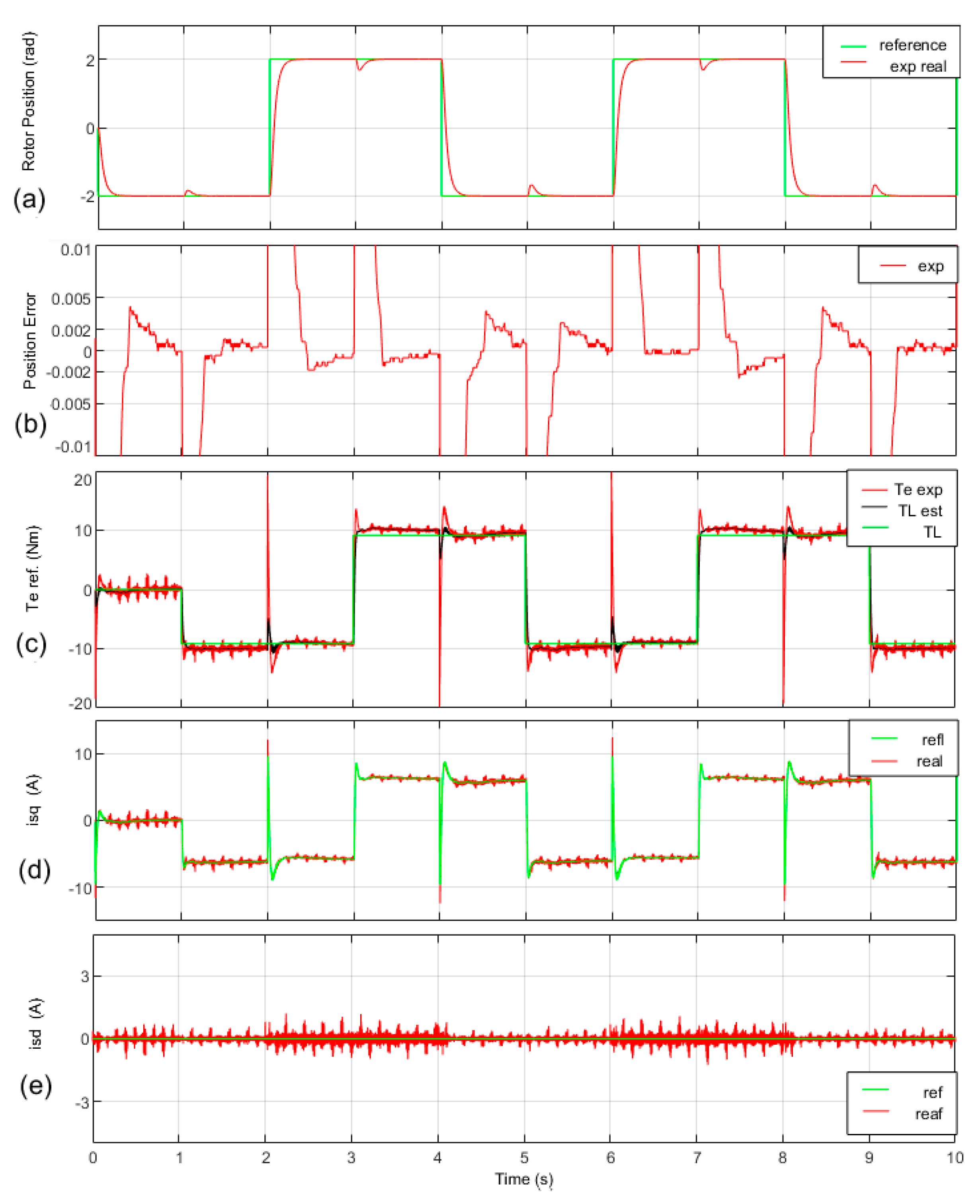
Figure 10 shows the experimental performance of the D2 position regulator for the PMSM machine. The test was the same as that employed and shown in Figure 5, but in this case using a square load torque of 9.15 N·m (75% of rated torque). Observing the response of the motor, it was fast and with small overshoot (a) and (b). The position error in the steady state was small or equal to 0.004 rad (0.2292°), obtaining excellent position tracking taking into account the hard load disturbance conditions. In spite of this, the electromagnetic torque, (c), was smooth, like its current, (d). The estimator of the load torque also worked very fine, obtaining a very similar disturbance’s waveform. Finally, it could be seen that the real rotor flux current, (e), tracked very properly its reference in these hard situations, obtaining that the machine produced only the magnet rotor flux successfully.
4. Conclusions
Taking into account the results obtained in the simulation and in the experimental tests, the next conclusions could be remarked. For three-phase machines of several units of kW, a very good position tracking was obtained employing a bandwidth (ωGCϴm) between 40 and 50 rad/s, and a phase margin (PMϴm) around of 70° for the PD regulator, when a step type position reference and the load torque was unknown and its value took up to 50% or less than the rated value of the electromagnetic torque. Really excellent results were obtained, with a position error of 0.007 rad (0.4011°) for IM and 0.002 rad (0.1146°) for PMSM. For load torque that was 75% or higher of the rated value of the electromagnetic torque, a bandwidth (ωGCϴm) between 75 and 85 rad/s, and a phase margin (PMϴm) around of 80° were necessary, obtaining also excellent results: a position error of 0.015 rad (0.8594°) for IM and between 0.004 rad (0.2292°) and 0, for PMSM. The PMSM motor provided better accuracy than the IM machine by employing the same PD position controller. The implementation of the load torque estimator was essential to obtain these results. Regarding the two PI inner loops, the tuning of a bandwidth (ωGCi) of 3000 rad/s and a phase margin (PMi) of 70°, was adequate for both loops (isd and isq), in both machines, due to that the current tracking was also very good in all cases. Moreover, despite PMSM having different stator inductances (Lsd and Lsq), the solution was to get their arithmetic mean value (Ls) and employ it in tuning for both loops, obtaining good results.
The methodology presented in this paper consists of a simple way to tune the position PD regulator for the most employed kind of commercial/industrial three-phase motors, that is IM and PMSM, obtaining excellent results, as well as much other advanced position controllers. This methodology could be used for other three-phase machines like Switched Reluctance Motor (SRM), Brushless DC (BLDC), Double Feed Induction Machine (DFIM) and including DC motors, for machines of different power.
Author Contributions
Conceptualization, P.A., O.B. and J.A.C.; Data curation, F.J.M.; Formal analysis, I.M. and F.J.M.; Investigation, P.A. and F.J.M.; Methodology, P.A., O.B., J.A.C. and I.M.; Software, O.B. and I.M.; Validation, P.A. and J.A.C.; Writing—original draft, P.A.; Writing—review & editing, O.B., J.A.C. and P.A. All authors have read and agreed to the published version of the manuscript.
Funding
This research was partially funded by the Basque Government through the project SMAR3NAK (ELKARTEK KK-2019/00051.
Acknowledgments
The authors wish to express their gratitude to the Basque Government, and to the UPV/EHU for supporting this work.
Conflicts of Interest
The authors confirm that there is not any conflict of interest with any institution or company.
References
- Vas, P. The Space-Vector method. In Electrical Machines and Drives: a Space-Vector theory approach, 1st ed.; Oxford University Press: Oxford, UK, 1992; Volume 1, pp. 32–125. [Google Scholar]
- Kume, T.; Iwakane, T. High-Performance Vector-Controlled AC Motor Drives: Applications and New Technologies. IEEE Trans. Ind. Appl. 1987, 23, 872–880. [Google Scholar] [CrossRef]
- Stojic, M.; Vukosavic, S. Design of microprocessor-based system for positioning servomechanism with induction motor. IEEE Trans. Ind. Electron. 1991, 38, 369–378. [Google Scholar] [CrossRef]
- Alkorta, P.; Barambones, O.; Cortajarena, J.A.; Vicandi, F.J.; Martija, I. Effective Proportional Derivative Position control of Induction Motor Drives. In Proceedings of the 2016 IEEE International Conference on Industrial Technology (ICIT), Taipei, Taiwan, 14–17 March 2016. [Google Scholar]
- Huang, T.; El-Sharkawi, M. High performance speed and position tracking of induction motors using multi-layer fuzzy control. IEEE Trans. Energy Convers. 1996, 11, 353–358. [Google Scholar] [CrossRef]
- Cecati, C. Position Control of the Induction Motor using a Passivity-based Controller. IEEE Trans. Ind. Appl. 2000, 36, 1277–1284. [Google Scholar] [CrossRef]
- Rodriguez, P.; Dumur, D. Generalized predictive control robustification under frequency and time-domain constraints. IEEE Trans. Control. Syst. Technol. 2005, 13, 577–587. [Google Scholar] [CrossRef]
- Veselić, B.; Peruničić-Draženović, B.; Milosavljevic, Č. High-Performance Position Control of Induction Motor Using Discrete-Time Sliding-Mode Control. IEEE Trans. Ind. Electron. 2008, 55, 3809–3817. [Google Scholar]
- Barambones, O.; Alkorta, P.; De Durana, J.M.G. A real-time estimation and control scheme for induction motors based on sliding mode theory. J. Frankl. Inst. 2014, 351, 4251–4270. [Google Scholar] [CrossRef]
- Callegaro, A.D.; Nalakath, S.; Srivatchan, L.N.; Luedtke, D.; Preindl, M. Optimization-Based Position Sensorless Control for Induction Machines. In Proceedings of the 2018 IEEE Transportation Electrification Conference and Expo (ITEC), Long Beach, CA, USA, 13–15 June 2018; pp. 460–466. [Google Scholar]
- Egiguren, P.A.; Echeverria, J.A.C.; Caramazana, O.B.; Lopez, I.M.; Alcorta, J.C. Poles Placement Position Control of Induction Motor Drives. In Proceedings of the IECON 2019—45th Annual Conference of the IEEE Industrial Electronics Society, Lisbon, Portugal, 14–17 October 2019. [Google Scholar]
- Ogasawara, S.; Akagi, H. Implementation and position control performance of a position-sensorless IPM motor drive system based on magnetic saliency. IEEE Trans. Ind. Appl. 1998, 34, 806–812. [Google Scholar] [CrossRef] [Green Version]
- Hua, Y.; Sumner, M.; Asher, G.; Gao, Q.; Saleh, K. Improved sensorless control of a Permanent Magnet Synchronous Machine using fundamental Pulse Width Modulation excitation. IET Electr. Power Appl. 2011, 5, 259–370. [Google Scholar] [CrossRef] [Green Version]
- Ghafari-Kashani, A.; Faiz, J.; Yazdanpanah, M. Integration of non-linear H∞∞ and sliding mode control techniques for motion control of a permanent magnet synchronous motor. IET Electr. Power Appl. 2010, 4, 267. [Google Scholar] [CrossRef]
- Yin, Z.; Gong, L.; Du, C.; Liu, J.; Zhong, Y. Integrated Position and Speed Loops Under Sliding-Mode Control Optimized by Differential Evolution Algorithm for PMSM Drives. IEEE Trans. Power Electron. 2019, 34, 8994–9005. [Google Scholar] [CrossRef]
- Lin, F.-J.; Lin, C.-H. A Permanent-Magnet Synchronous Motor Servo Drive Using Self-Constructing Fuzzy Neural Network Controller. IEEE Trans. Energy Convers. 2004, 19, 66–72. [Google Scholar] [CrossRef]
- Lin, F.-J.; Sun, I.-F.; Chang, J.-K.; Yang, K.-J. Intelligent position control of permanent magnet synchronous motor using recurrent fuzzy neural cerebellar model articulation network. IET Electr. Power Appl. 2015, 9, 248–264. [Google Scholar] [CrossRef]
- Yu, J.; Shi, P.; Yu, H.; Chen, B.; Lin, C. Approximation–based Discrete-time Adaptive Position Tracking Control for Interior Permanent Magnet Synchronous Motors. IEEE Trans. Cybernetics. 2015, 45, 1363–1371. [Google Scholar] [CrossRef] [PubMed]
- Belda, K.; Vosmik, D. Explicit Generalized Predictive Control of Speed and Position of PMSM Drives. IEEE Trans. Ind. Electron. 2016, 63, 3889–3896. [Google Scholar] [CrossRef]
- Mubarok, M.S.; Liu, T.-H. Implementation of Predictive Controllers for Matrix-Converter-Based Interior Permanent Magnet Synchronous Motor Position Control Systems. IEEE Trans. Emerg. Sel. Topics Power Electron. 2019, 7, 261–273. [Google Scholar] [CrossRef]
- Mohan, N. Mathematical Description of Vector Control in Induction Machines; Wiley: Hoboken, NJ, USA, 2014; Volume 1, pp. 79–96. [Google Scholar]
- Bose, B.K. AC Machines for Drives. In Modern Power Electronics and AC Drives, 1st ed.; Prentice Hall PTR: Upper Saddle River, NJ, USA, 2002; Volume 1, pp. 86–92. [Google Scholar]
Figure 1.
The proportional derivative position indirect vector control scheme for the three-phase motor.
Figure 1.
The proportional derivative position indirect vector control scheme for the three-phase motor.

Figure 2.
Simplified scheme for proportion derivative (PD) position indirect vector control for the three-phase motor.
Figure 2.
Simplified scheme for proportion derivative (PD) position indirect vector control for the three-phase motor.

Figure 3.
Simplified scheme for PD position control with Feed-Forward (FF) action for the three-phase motor.
Figure 3.
Simplified scheme for PD position control with Feed-Forward (FF) action for the three-phase motor.
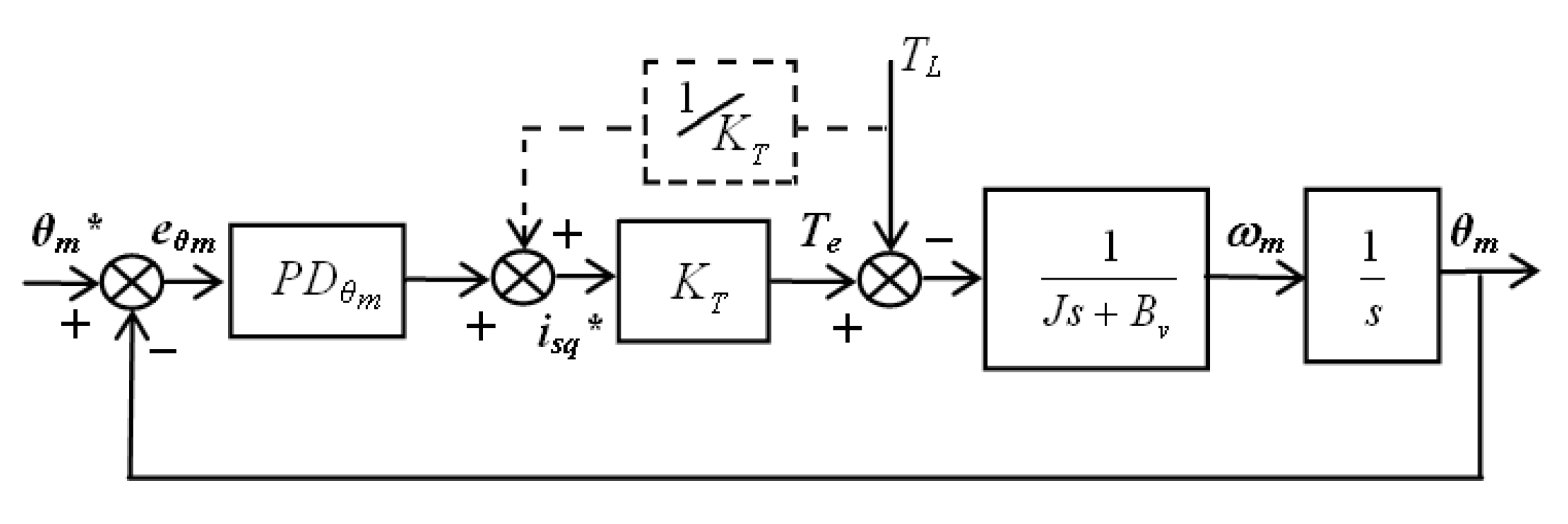
Figure 4.
Simplified scheme of the PI regulator for isq and isd currents loops (induction motor (IM) machine case).
Figure 4.
Simplified scheme of the PI regulator for isq and isd currents loops (induction motor (IM) machine case).
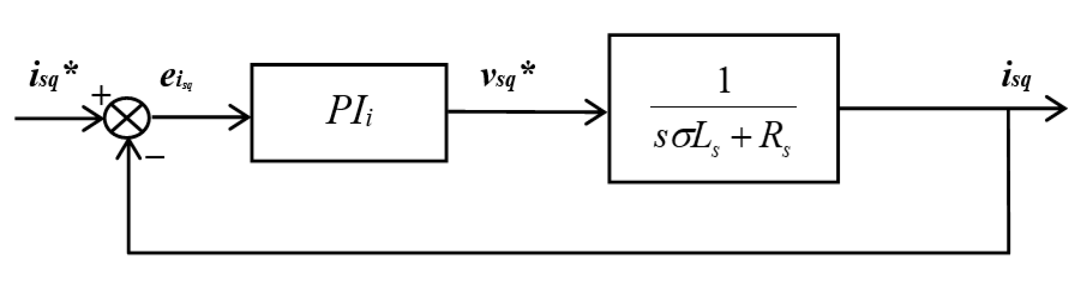
Figure 5.
Simplified scheme of the PI regulator for isq and isd currents loops (permanent magnet synchronous motor (PMSM) machine case).
Figure 5.
Simplified scheme of the PI regulator for isq and isd currents loops (permanent magnet synchronous motor (PMSM) machine case).
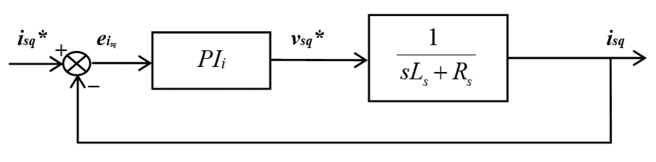
Figure 6.
(a) IM tests bench and (b) PMSM tests bench.
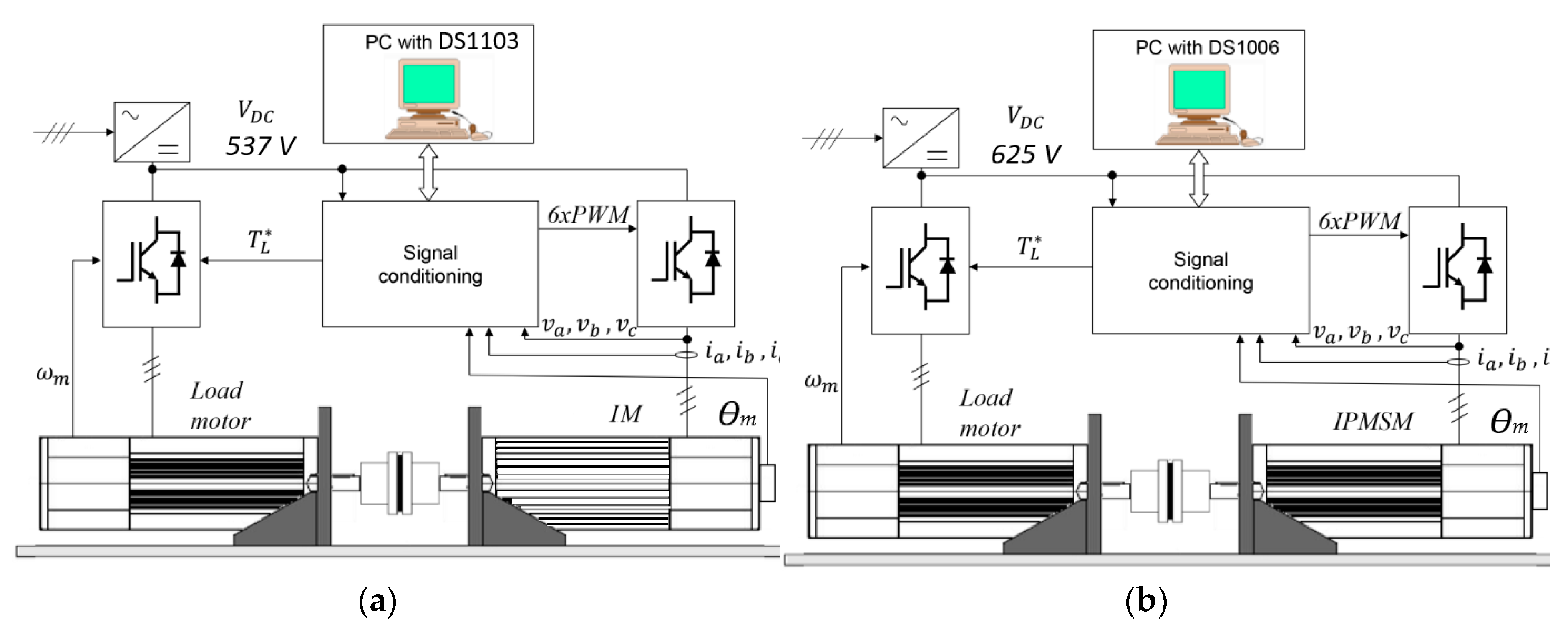
Figure 7.
Simulation and experimental tests’ performances employing the D1 design for the IM machine: (a) rotor position, reference and real (rad); (b) rotor position error (rad); (c) rotor position error zoom (rad); (d) rotor speed (rad/s); (e) electromagnetic torque (Te), estimated load torque (TL est) and load torque (TL), (N·m); (f) torque current, isq (A) and (g) rotor flux current, reference and real, isd (A).
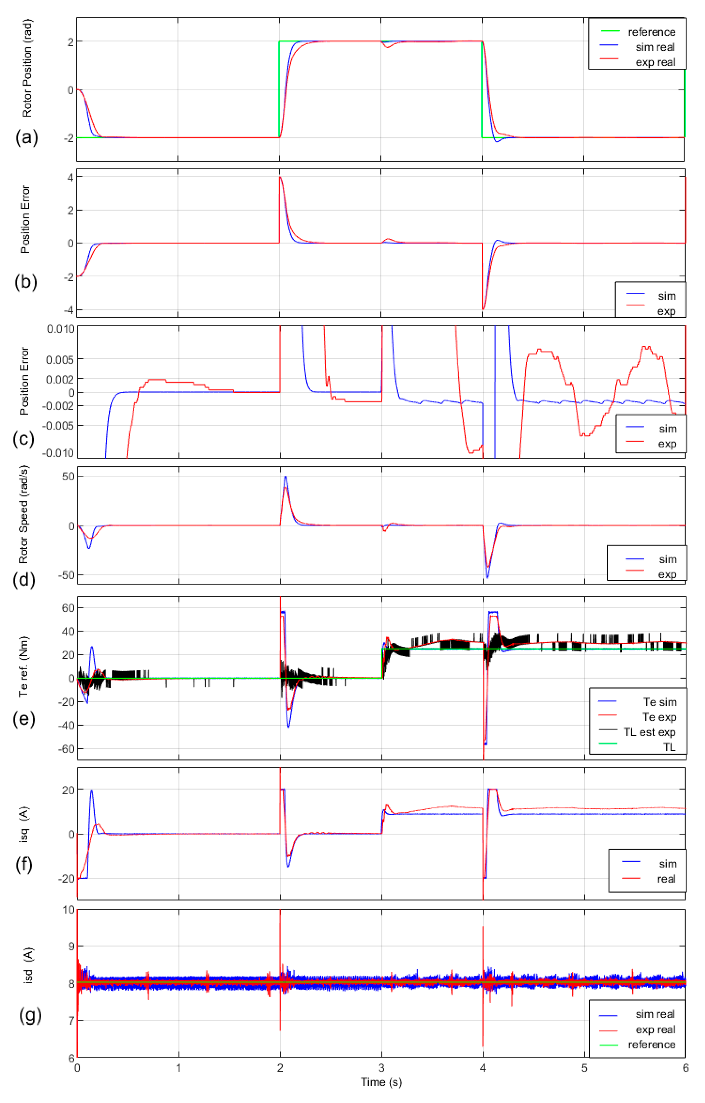
Figure 8.
Experimental test employing the D2 design for the IM machine: (a) rotor position, reference and real (rad); (b) rotor position error (rad); (c) rotor position error zoom (rad); (d) electromagnetic torque (Te), estimated load torque (TL est) and load torque (TL), (N·m); (e) torque current, isq (A) and (f) rotor flux current, reference and real, isd (A).
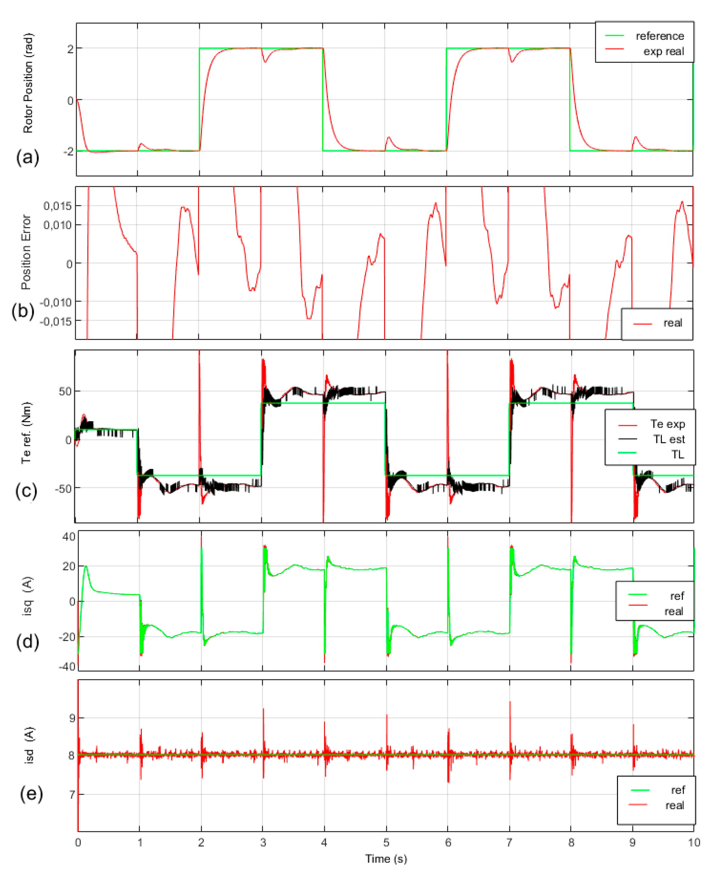
Figure 9.
Simulation and experimental tests’ performances employing the D1 design for the PMSM machine: (a) rotor position, reference and real (rad); (b) rotor position error (rad); (c) rotor position error zoom (rad); (d) rotor speed (rad/s); (e) electromagnetic torque (Te), estimated load torque (TL est) and load torque (TL), (N·m); (f) torque current, isq (A); (g) rotor flux current, reference and real, isd (A).

Figure 10.
Experimental test employing the D2 design for the IM machine: (a) rotor position, reference and real (rad); (b) rotor position error (rad); (c) rotor position error zoom (rad); (d) electromagnetic torque (Te), estimated load torque (TL est) and load torque (TL), (N·m); (e) torque current, isq (A) and (f) rotor flux current, reference and real, isd (A)

Table 1.
D1 and D2 position controller designs for the IM machine.
| Design | ωGCϴm | PMϴm | ωGCi | PMi |
|---|---|---|---|---|
| D1 | 50 rad/s Kpϴm = 11.1, | 74° Kdϴm = 914.63, | 3000 rad/s Kpi = 10.82, | 70° Kii = 14401 |
| D2 | 85 rad/s Kpϴm = 15.23, | 79° Kdϴm = 1597, | 3000 rad/s Kpi = 10.82, | 70° Kii = 14401 |
Table 2.
D1 and D2 position controller designs for the PMSM machine.
| Design | ωGCϴm | PMϴm | ωGCi | PMi |
|---|---|---|---|---|
| D1 | 45 rad/s Kpϴm = 2.8, | 70° Kdϴm = 139.25, | 3000 rad/s Kpi = 15, | 70° Kii = 18004 |
| D2 | 75 rad/s Kpϴm = 4.25, | 75° Kdϴm = 248.15, | 3000 rad/s Kpi = 15, | 70° Kii = 18004 |
© 2020 by the authors. Licensee MDPI, Basel, Switzerland. This article is an open access article distributed under the terms and conditions of the Creative Commons Attribution (CC BY) license (http://creativecommons.org/licenses/by/4.0/).
Share and Cite
MDPI and ACS Style
Alkorta, P.; Barambones, O.; Cortajarena, J.A.; Martija, I.; Maseda, F.J. Effective Position Control for a Three-Phase Motor. Electronics 2020, 9, 241. https://doi.org/10.3390/electronics9020241
AMA Style
Alkorta P, Barambones O, Cortajarena JA, Martija I, Maseda FJ. Effective Position Control for a Three-Phase Motor. Electronics. 2020; 9(2):241. https://doi.org/10.3390/electronics9020241
Chicago/Turabian StyleAlkorta, Patxi, Oscar Barambones, José Antonio Cortajarena, Itziar Martija, and Fco. Javier Maseda. 2020. "Effective Position Control for a Three-Phase Motor" Electronics 9, no. 2: 241. https://doi.org/10.3390/electronics9020241
Note that from the first issue of 2016, this journal uses article numbers instead of page numbers. See further details here.