Investigation of Induced Charge Mechanism on a Rod Electrode

Abstract

Rod electrodes based on an electrostatic induction mechanism are widely used in various industrial applications, but the analytic solution of an induced charge mechanism on a metal rod electrode has not yet been systematically established. In this paper, the theoretical model of the induced charge on a rod electrode is obtained through the method of images. Then, the properties of the rod electrode under the action of the point charge are studied, including the induced charge density distribution on the rod electrode, the amount of the induced charge with different diameters and lengths of the electrode, and the effective space region induced by the electrode. On this basis, a theoretical model of the induced current on a rod electrode is established, which is used to study the induced current properties by a moving point charge. It is found that both the magnitude and bandwidth of the induced current increase with the increased point charge velocity. Finally, three experimental studies are conducted, and the experimental results show good consistency with the analysis of the theoretical model, verifying the correctness, and accuracy of the model. In addition, the induced charge mechanism studied in this paper can act as an effective basis for the rod electrode sensor design in terms of the optimal radius and length.

1. Introduction

Dust pollution is a common issue in industrial and mining enterprises, such as coal mining, iron mining, etc. [1,2]. Dust moves together with the ventilation air and settles on walls and equipment. Dust in the ventilation air can have negative effects on the working conditions, posing a risk to the health of workers. Many measures have been taken to improve the air quality [3,4]. Real-time and accurate detection of the dust concentration is a basic guarantee to ensure an effective dust removal [5,6].

Based on the electrostatic induction phenomenon, electrodes are widely used to measure the electric charges carried on solid particles, mass flow rate, concentration, volume loading, mean flow velocity, and other electrical and mechanical parameters in two-phase and multiphase gas–solid flows such as those in pneumatic conveyances, in the air, etc. [7]. When charged particles move close to or away from a metal electrode, a charge with the opposite polarity to the dust particles is induced on the surface of the electrode. Hence, the physical parameters of the charged particles can be acquired by measuring the characteristics of the induced charge on the electrode. In practical applications, metal electrodes are fabricated in different shapes to acquire different measurement parameters in various environments. Typical electrodes mainly include the ring, curved, square, and rod electrodes and arrays composed of electrodes of different shapes.

The ring electrode has received wide attention by researchers because of its noninvasive characteristics. It is an electrode form with relatively mature theory and applications. Weinheimer [8] derived a charge numerical solution on the surface of ring electrodes induced by the point charge, which was applied to the measurement of meteorological precipitation charge. Yan, Gajewski, and Woodhead used a correlation method to measure velocity after studying the sensing mechanism, spatial sensitivity, and spatial filtering effect of noninvasive ring induction electrodes [9,10,11]. In recent years, ring charge-sensing sensors have been widely utilized in the measurement of dilute phase/dense phase of gas–solid two-phase flow parameters [12,13,14]. At the same time, some modern signal processing algorithms have further improved the measurement accuracy [15,16,17,18,19]. For example, Wang et al. [20] improved the measurement accuracy by applying the wavelet transform to the multiphase flow parameters. Considering that the signal measured by the ring electrode is an average feature over the entire cross-section, Zhang, Yang, and Dong’s research found that the arc-shaped sensing electrode had an advantage in particle velocity and concentration distribution measurement in the monitoring of particle motion in gas–solid fluidized beds [21,22,23]. Qian also combined arc-shaped electrodes with digital images for the measurement of biomass–coal particles in fuel-injection pipelines [24]. Liu and Yao obtained the characteristics of square electrodes through theoretical and simulation studies, and utilized them on a square pneumatic conveying pipeline [25,26]. Compared with the above two models, Zhang used the method of images to obtain a simple analytical solution of the square electrode [27]. With the increasing complexity of the measurement environment, combinations of multistatic sensors and even electrostatic sensor arrays are applied to acquire different parameters of various pipelines [28,29].

Rod sensors based on the electrostatic induction mechanism have been widely used in industrial fields [7,30], mainly due to their simpler installation compared to other types of sensors, its working principle, and its applications in the real world are shown as Figure 1. Since they can accurately reflect pollutant emissions such as the steel mill flue gas, they have been widely applied for the detection of particulate matter concentration and dust in dust collector bags. Although the noninvasiveness is a great advantage of the ring electrodes, it usually takes the form of a spool piece installed in line with the pipe, which leads to an expensive and challenging installation. Moreover, signals collected by the ring electrodes are an overall result of the induced signals, making it difficult to detect local flow regimens. In comparison to the ring electrodes, the installation of rod electrodes is easier, since they only need a suitable drilling hole at any position of the pipe, making it possible to detect local flow regimes [30]. Therefore, rod electrodes are widely used in industrial areas and some research work has been performed. Shao compared the advantages and disadvantages of the ring electrode and rod electrode electrostatic sensors in measuring the pulverized coal speed [31,32], and proved that both types of electrodes achieved the same measurement accuracy in the coal dust measurement.

Electrostatic induction is a basic physical phenomenon in which the opposite induced charge is induced on the conductor if the point charge is close to the conductor. It is a qualitative conclusion. However, the analytic solution of the amount of induced charge when the point charge is close to the conductor has always been a difficult problem. It is a physical boundary value problem, which is difficult to represent with an analytical solution. The common method is to solve the Poisson equation through numerical calculations to get the amount of induced charge on the electrode. Krabicka studied the characteristics of electrostatic charges on rod electrodes by the finite element analysis (FEA) method and obtained an approximate solution [30]. However, this method requires remodeling of rod sensing electrodes of different lengths and diameters, which increases the modeling time. The simulation of large sensing electrodes takes too much time and the simulation accuracy is heavily dependent on the simulation software such as COMSOL. Therefore, this method is limited in practical application. Chen [33] established a mathematical model of rod electrodes by a theoretical derivation, but the fact that the induction conductor is a metal conductor was neglected, and the metal conductor was modeled as an insulator.

Analytic solutions of rod electrodes can be used to optimize the sensor design or interpret how particles at various locations influence the signal; for example, the bandwidth and amplitude. In order to establish a simple and easy-to-use mathematical model of rod electrodes, the method of images and the symmetry of rod electrodes are employed in this paper. The mathematical formula of the amount of charge induced by the point charge on the sensing rod electrode is obtained, and the equation is then used to study the physical properties of the sensing electrode under the action of the point charge. Based on this model, the distribution characteristics of the induced charge on the surface of the electrode and the influence of the electrode length on the induced charge density are studied, the induced charge of the induced electrode is simulated when the point charge moves in different directions, the amount of the induced current on the sensing electrode is studied, the spectral characteristics and the influence of the general measurement model of the induced current are analyzed, the experimental model is established, and the validity and accuracy of the model are verified by experiments.

2. Induced Charge Model on Rod Electrode by Point Charge

The method of images is an indirect method to solve the electrostatic field problem by applying the uniqueness theorem. The electrostatic method can be used to treat the actual partitioned uniform medium as uniform, and replace the actual complex charge distribution on the boundary with a simple charge distribution on the virtual closed setting boundary of the research field for calculation. According to the uniqueness theorem, this result is correct as long as the electric field generated by the imaginary charge together with the actual charge within the boundary satisfies a given boundary condition [34].

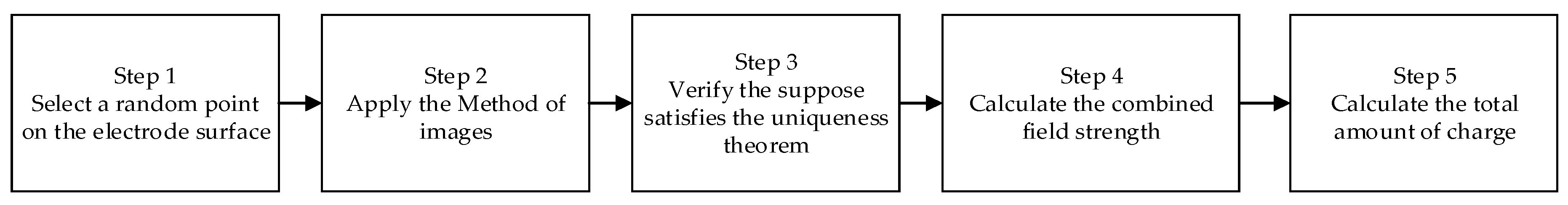
In this paper, the relationship between the rod electrode and point charge $q$ is established by the method of images, which mainly models the relationship of the induced charge by the point charge $q$ with two basic parameters of the rod electrode, length, and radius. The steps of the proposed method to model the induced charge on a rod electrode is shown in Figure 2. The following subsections explains the steps in detail step by step.

2.1. Step 1 Select A Random Point On the Electrode Surface

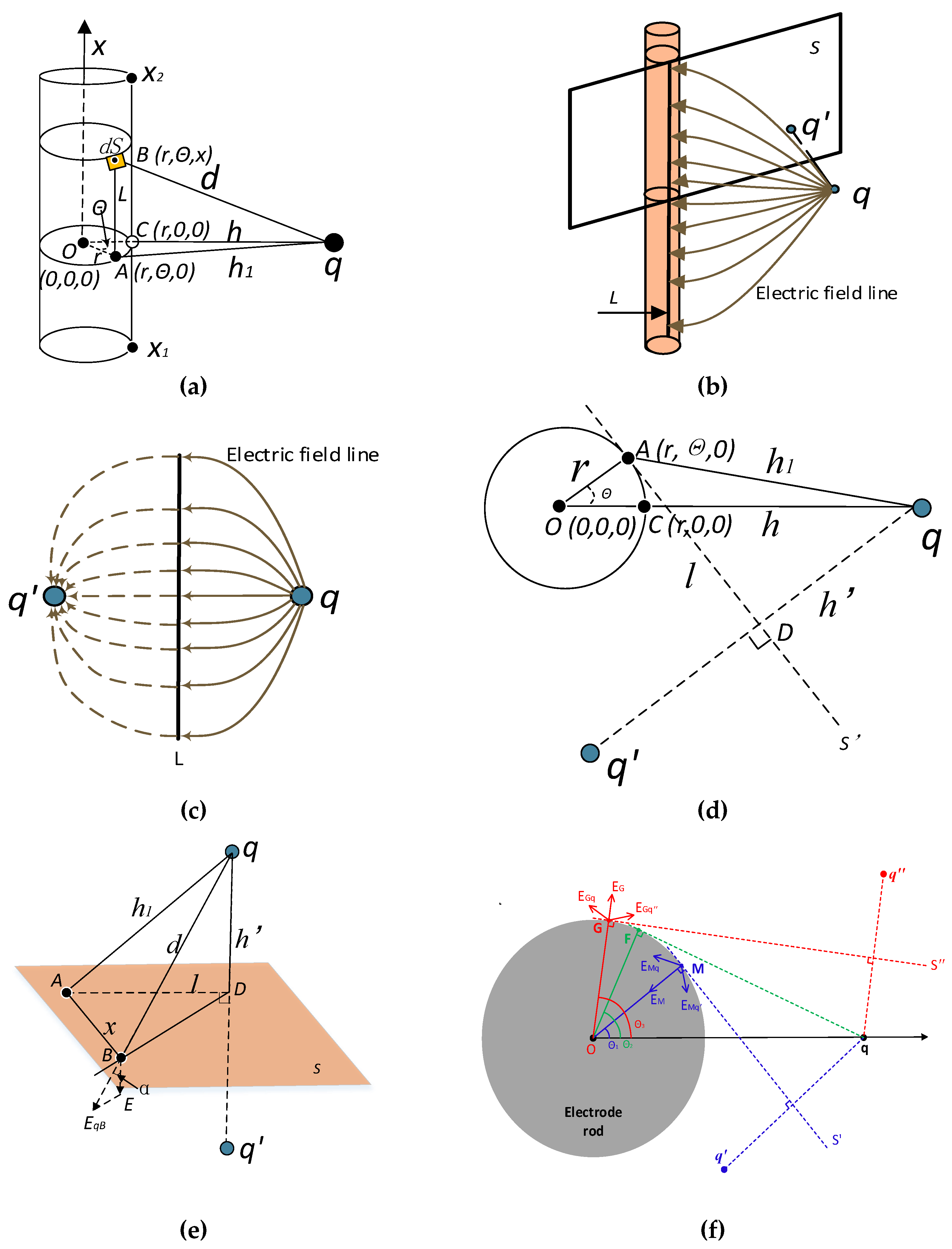
To model the induced current on a rod electrode by a point charge, a cylindrical coordinate system is established, as shown Figure 3a, with the origin point $O$ being the center of the electrode. Point C is the intersection of Oq and the electrode’s surface, point $A$ is one point on the surface of the electrode, and plane OAC is perpendicular to line L. Suppose $\theta$ is the angle between line $OA$ and line $OC$, the coordinate of point $A$ can be written as $\left(r,\theta ,0\right)$. Point charge $q$ is in plane $OAC$ and is located on the extension line of $OC$, and the distance to $C$ is $h$ and the distance to point $A$ is $h_1$. Point $B$ is a random point on the electrode surface and $x$ is the vertical distance from B to plane $OAC$, hence the coordinates of point $B$ are $\left(r,\theta ,x\right)$.

2.2. Step 2 Apply the Method of Images

In addition to the electric field caused by point charge q in the electrolyte, the effect of the induced charge on the rod electrode should also be considered. However, the electric field distribution on the sensing electrode is unknown, which is the problem that this paper needs to solve. As shown in Figure 3b, it is assumed that an infinitely large plane $S$ is tangent to the metal rod electrode and the intersection between the rod electrode and plane $S$ forms a straight line $L$. The electric field intensity $E$ and the electric field line distribution generated on infinite plane $S$ can be obtained by the method of images, as shown in Figure 3c. Note that these electric field lines are perpendicular to the surface of the rod electrode. It is assumed that electric field E on line L of infinite plane S formed by point charge q is electric field E on the line of the rod electrode. Then, the image method is assumed to have a point charge at q′ with an equivalent charge (−q) to point charge q.

2.3. Step 3 Verify the Suppose Satisfies the Uniqueness Theorem

After removing the electrode and conductive plate S, and the following conditions are still satisfied:

(1)

In addition to the position where the point charge is located, ${\nabla }^2\phi =0$ is satisfied everywhere, and $\phi$ is the potential.

(2)

Taking infinity as the reference point, the potential at the interface between the medium and conductor L is zero.

(3)

The direction of the electric field line is unchanged, which is the direction of the vertical electrode surface pointing to the axis.

These conditions satisfy the uniqueness theorem.

2.4. Step 4 Calculate the Combined Field Strength

By applying the method of images, we can obtain the electric field intensity $E$ of point $B$. A cross-section view of plane $OAC$ is illustrated in Figure 3d; the projection of point $B$ is point $A$ and the projection of plane $S$ is line $S^{\prime }$. The connecting line between point charge $q$ and image charge $q^{\prime }$ intersects with $S^{\prime }$ at point $D$, the distance between point $A$ and point $D$ is $l$, and the distance between point $q$ and point $D$ is $h^{\prime }$; $d$ is the distance between point charge $q$ and B.

The mathematical expressions of $h^{\prime }$, $l$, and $h_1$ and the range of values of $\theta$ can be obtained, as follows:

$$h^{\prime }=\left(h-\left(\frac{r}{cos\theta }-r\right)\right)cos\theta$$

(1)

$$l=rtan\theta +h^{\prime }tan\theta$$

(2)

$$h_1={(h^{\prime }{}^2+l^2)}^{1/2}$$

(3)

$$d={(h_1{}^2+x^2)}^{1/2}.$$

(4)

To determine the range of $\theta$, suppose point charge q carries a positive charge and is located at a position with minimum distance h to the surface of the electrode, as shown in Figure 3f. F is at the intersection of the tangential line through point charge q, and the angle ${\theta }_2$ is equal to $acos\left(r/\left(r+h\right)\right)$.

For any point M at a position that satisfies the condition ${\theta }_1<acos\left(r/\left(r+h\right)\right)$, its electric field strength can be analyzed as follows. According to the method of images, the imaginary charge is $q^{\prime }$, carrying a negative charge. $E_{Mq}$ is the electric field strength generated by point charge $q$, and $E_{M{q}^{\prime }}$ is the electric field strength generated by point charge $q^{\prime }$. Their synthetic electric field of strength is $E_M$, which points to the center point O. The orientation of $E_M$ conforms with the electric field on the metal being perpendicular to the metal surface. As is known, if the charge of $q$ is positive, the induced charge on the metal surface should be negative. This further confirms the correctness of the orientation of $E_M$.

For any point G at a position that satisfies the condition ${\theta }_3>acos\left(r/\left(r+h\right)\right)$, its electric field strength can be analyzed similarly. According to the method of images, the imaginary charge is $q^{″}$, also carrying a negative charge. $E_{Gq}$ is the electric field strength generated by point charge $q$, and $E_{G{q}^{″}}$ is the electric field strength generated by point charge $q^{″}$. The synthetic field of strength is $E_G$, which points to a direction off the center O and is perpendicular to the metal surface. This indicates that the charge at point G is positive, which does not comply with the induced charge being negative. Hence, such a point should not have an induced charge generated from point charge $q$.

According to the above analysis, $\theta$ should not be larger than $acos\left(r/\left(r+h\right)\right)$. Using the same method, we can get that the minimum value of $\theta$ is not smaller than $-acos\left(r/\left(r+h\right)\right)$.

In summary, the range of $\theta$ can be determined as the following when the method of images is used:

$$\theta =\left[-acos\left(\frac{r}{r+h}\right), acos\left(\frac{r}{r+h}\right)\right]$$

(5)

It can be seen from Figure 3e that field strength $E_{qB}$ is the summation result of point charge $q$ and its image $q^{\prime }$. $E_{qB}$ can be expressed as

$$E_{qB}=2\frac{q}{4\pi {\epsilon }_0{d}^2}$$

(6)

and $E$ can be expressed as

$$E=E_{qB}cos\alpha .$$

(7)

Electric field strength $E$ of point B based on the method of images can be obtained as

$$E=\frac{q{h}^{\prime }}{2\pi {\epsilon }_0{d}^{3/2}}$$

(8)

where ${\epsilon }_0$ is the vacuum permittivity.

2.5. Step 5 Calculate the Total Amount of Charge

The charge density $\rho$ of point B is obtained as

$$\rho =-{\epsilon }_{0}E=\frac{-q{h}^{\prime }}{2\pi d^{3/2}}$$

(9)

The $dS$ marked in orange on the surface of the electrode contains point B, as in Figure 3c; the area of $dS$ is expressed as

$$dS=rd\theta dx$$

(10)

When $d\theta$ and $dx$ are infinite to zero, the charge density of $dS$ will be the density of point B.

The total amount of the induced charge on the metal electrode is obtained:

$$Q=\oint \rho dS=\underset{x_1}{\overset{x_2}{{\displaystyle \int }}}\underset{-acos\left(\frac{r}{r+h}\right)}{\overset{acos\left(\frac{r}{r+h}\right)}{{\displaystyle \int }}}\frac{-q{h}^{\prime }r}{2\pi d^{3/2}}d\theta dx$$

(11)

where $x_1$, $x_2$ are the x-coordinates of the ends of the metal electrode.

By changing the order of the integration, we get

$$Q=\underset{-acos\left(\frac{r}{r+h}\right)}{\overset{acos\left(\frac{r}{r+h}\right)}{{\displaystyle \int }}}\underset{x_1}{\overset{x_2}{{\displaystyle \int }}}\frac{-q{h}^{\prime }r}{2\pi d^{3/2}}dxd\theta .$$

(12)

The result is obtained as

$$Q={{\displaystyle \int }}_{-acos\left(\frac{r}{r+h}\right)}^{acos\left(\frac{r}{r+h}\right)}\left(\frac{-qr{h}^{\prime }{x}_2}{2\pi h_1{}^2{\left(h_1{}^2+x_2{}^2\right)}^{\raisebox{1ex}{$1$}\!\left/ \!\raisebox{-1ex}{$2$}\right.}}-\frac{-qr{h}^{\prime }{x}_1}{2\pi h_1{}^2{\left(h_1{}^2+x_1{}^2\right)}^{\raisebox{1ex}{$1$}\!\left/ \!\raisebox{-1ex}{$2$}\right.}}\right)d\theta .$$

(13)

Let the charge distribution function along with $x_1,x_2 \mathrm{and} \theta$ be $F\left(x_1,x_2,\theta \right)$:

$$F\left(x_1,x_2,\theta \right)=\frac{-qr{h}^{\prime }{x}_2}{2\pi h_1{}^2{\left(h_1{}^2+x_2{}^2\right)}^{\raisebox{1ex}{$1$}\!\left/ \!\raisebox{-1ex}{$2$}\right.}}-\frac{-qr{h}^{\prime }{x}_1}{2\pi h_1{}^2{\left(h_1{}^2+x_1{}^2\right)}^{\raisebox{1ex}{$1$}\!\left/ \!\raisebox{-1ex}{$2$}\right.}}.$$

(14)

When point charge $q$ moves infinitely away from the electrode, the amount of induced charge is $\underset{h\to \infty }{lim}Q=0$. This means the amount of the induced charge generated by the point charge at infinity on the rod-shaped metal electrode is zero. From the analysis of Section 3.2.1, it can been seen that when point charge $q$ is infinitely close to the electrode, the amount of the induced charge is $\underset{h\to 0}{lim}Q=-q$; that is, the amount of the induced charge generated on the rod-shaped metal electrode is $-q$ when the point charge is infinitely close to the metal electrode.

3. Characteristics of Induced Charge on a Rod Electrode

In this section, the basic characteristics of the induced charge on a rod electrode are analyzed by utilizing the model obtained in Section 2.

3.1. Induced Charge Distribution under the Effect of Point Charge

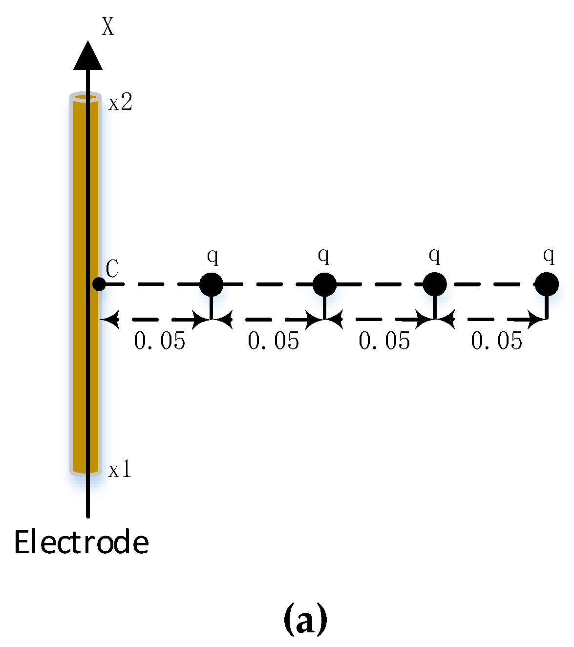
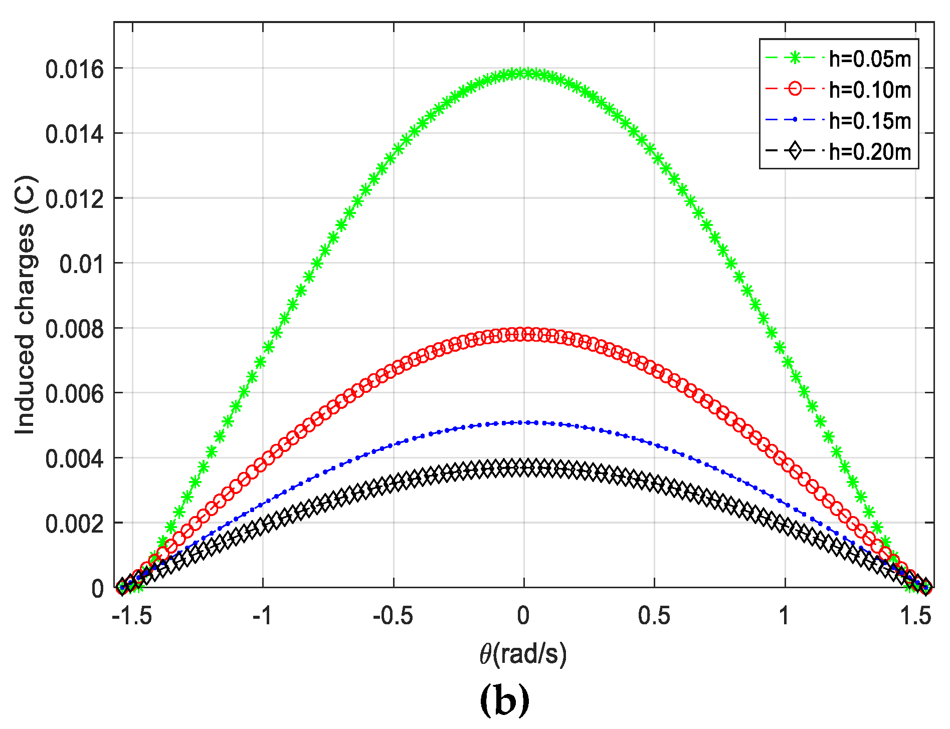
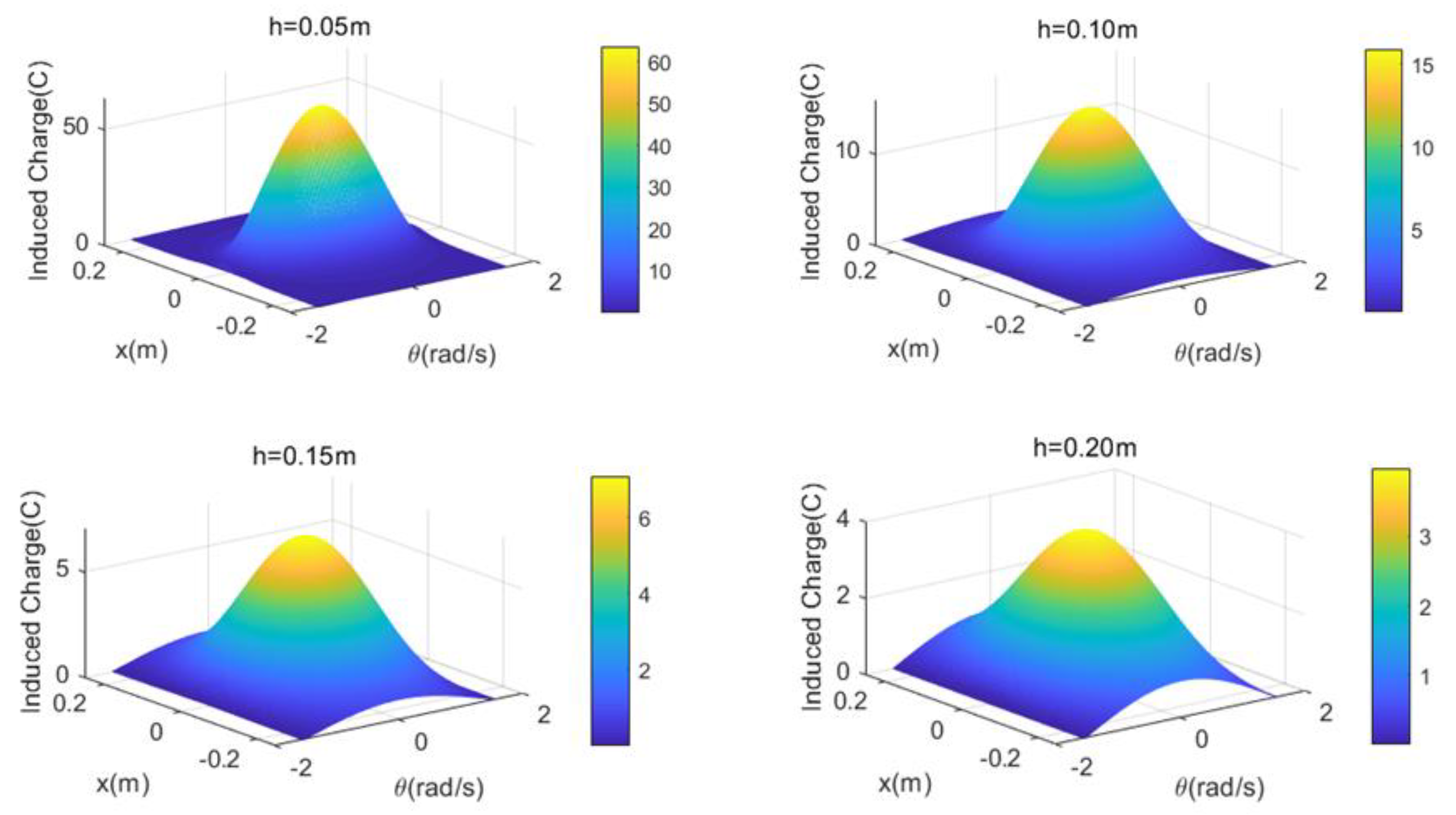
The induced charge distribution with $\theta$ is studied. Four cases of $h$ are studied, as shown in Figure 4a, where $h$ is selected as $0.05\mathrm{m}$, $0.10\mathrm{m}$, $0.15\mathrm{m}$, and $0.20\mathrm{m}$. The diameter of the electrode is $r=0.005 \mathrm{m}$, the length of the rod electrode is $0.50 \mathrm{m}$, and the two ends of the electrode are $x_1$ = $-0.25\mathrm{m}$ and $x_2$ = $0.25\mathrm{m}$. Charge $\mathrm{q}$ carries a charge quantity of $-1 \mathrm{C}$. Figure 4b shows the charge distribution with $\theta$. It can be observed that the charge decreases as distance $h$ increases and the charge reaches a maximum value when $\theta =0$.

The variation of the induced charge along $\left(\theta ,x\right)$ on the electrode is shown in Figure 5. The induced charge reaches its maximum value at the point $\left(r,0, 0\right)$. If the point charge is closer to the electrode, the charge distribution is more concentrated. When the sensing range $x$ is smaller, the induced charge is greater. This indicates that the closer the point charge is to the rod electrode, the more charge is induced in the small sensing region, and the charge distribution tends to gradually decrease when the distance from the point $\left(r,0, 0\right)$ increases.

3.2. Quantity of Charge Induced by Moving Point Charge

3.2.1. Effect of Distance between Electrode and Point Charge

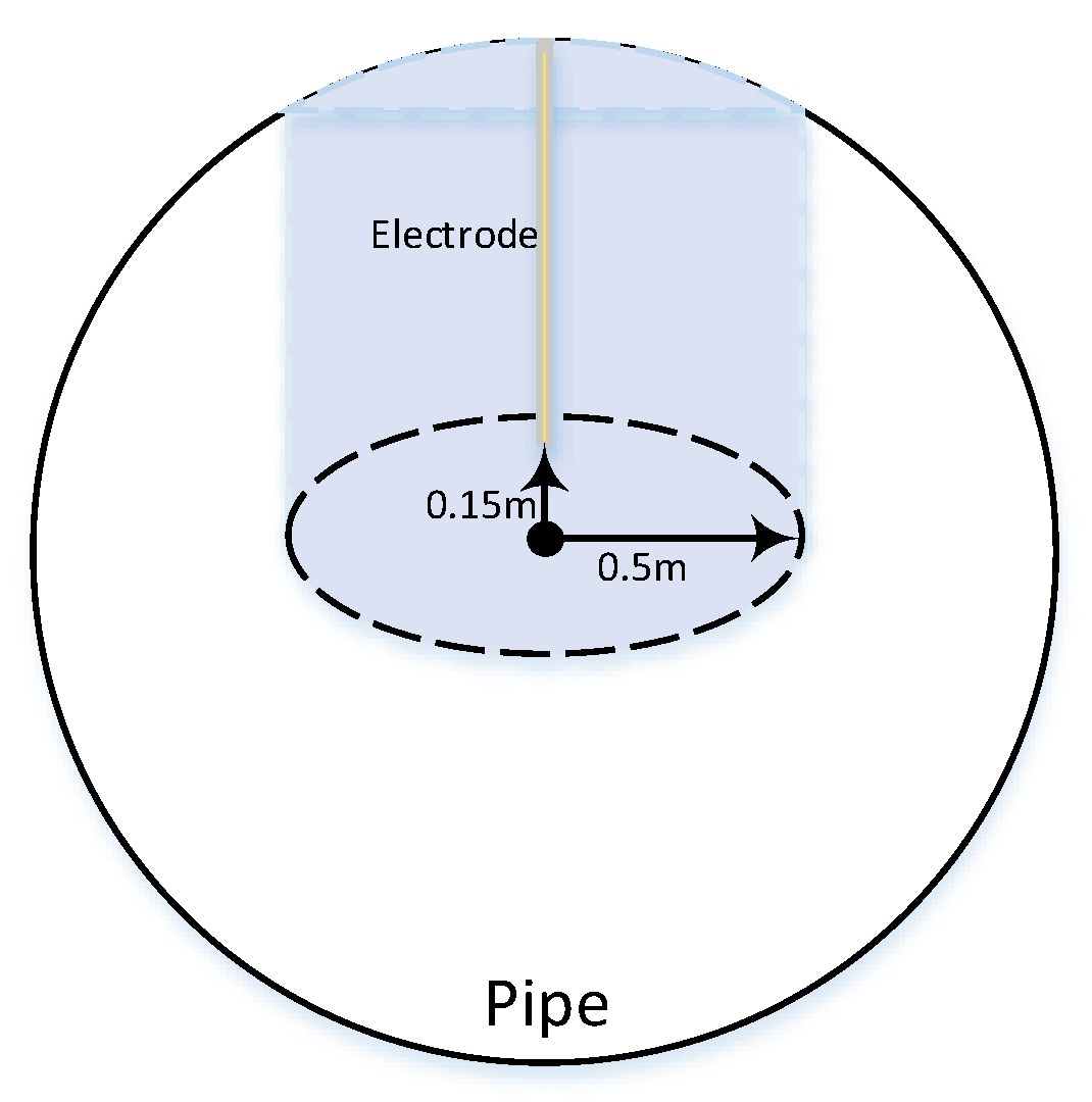
As shown in Figure 6a, the point charge $q$ carries −1 C charge and moves at a constant velocity of $5 \mathrm{m}/\mathrm{s}$ along the direction parallel to the pipeline and perpendicular to the electrode’s axis. The length of the electrode is $0.1 \mathrm{m}$ and the radius of electrode $r$ is $0.005\mathrm{m}$.

Suppose the distance between the electrode and point charge is $h$. We performed simulations on five distances, as presented in Figure 6b, showing the cross-section of the pipeline that contains the electrode. The distances between the surface of the electrode and the five positions of $\mathrm{A},\mathrm{B},\mathrm{C},\mathrm{D},\mathrm{E}$ are $0.1\mathrm{m}$, $0.2\mathrm{m}$, $0.3\mathrm{m}$,$0.4\mathrm{m}$, and $0.5\mathrm{m}$, respectively. The variations of the amount of charge induced on the electrode by these five simulations are shown in Figure 6c. Here, we define the distance from the point charge before it passes through points $\mathrm{A},\mathrm{B},\mathrm{C},\mathrm{D},\mathrm{E}$ as negative and the distance after as positive. It can be observed that the amount of charge decreases when the distance between the electrode and point charge increases. This applies when the distance between the electrode and point charge is within the range of $-0.5\mathrm{m}$ to $0.5\mathrm{m}$, and the amount of the induced charge can be neglected when it falls outside of this range Therefore, if there are charged particles uniformly distributed around the electrode, it can be considered that the induced charge on the electrode is generated by charges within a cylindrical section with a radius of $0.5\mathrm{m}$.

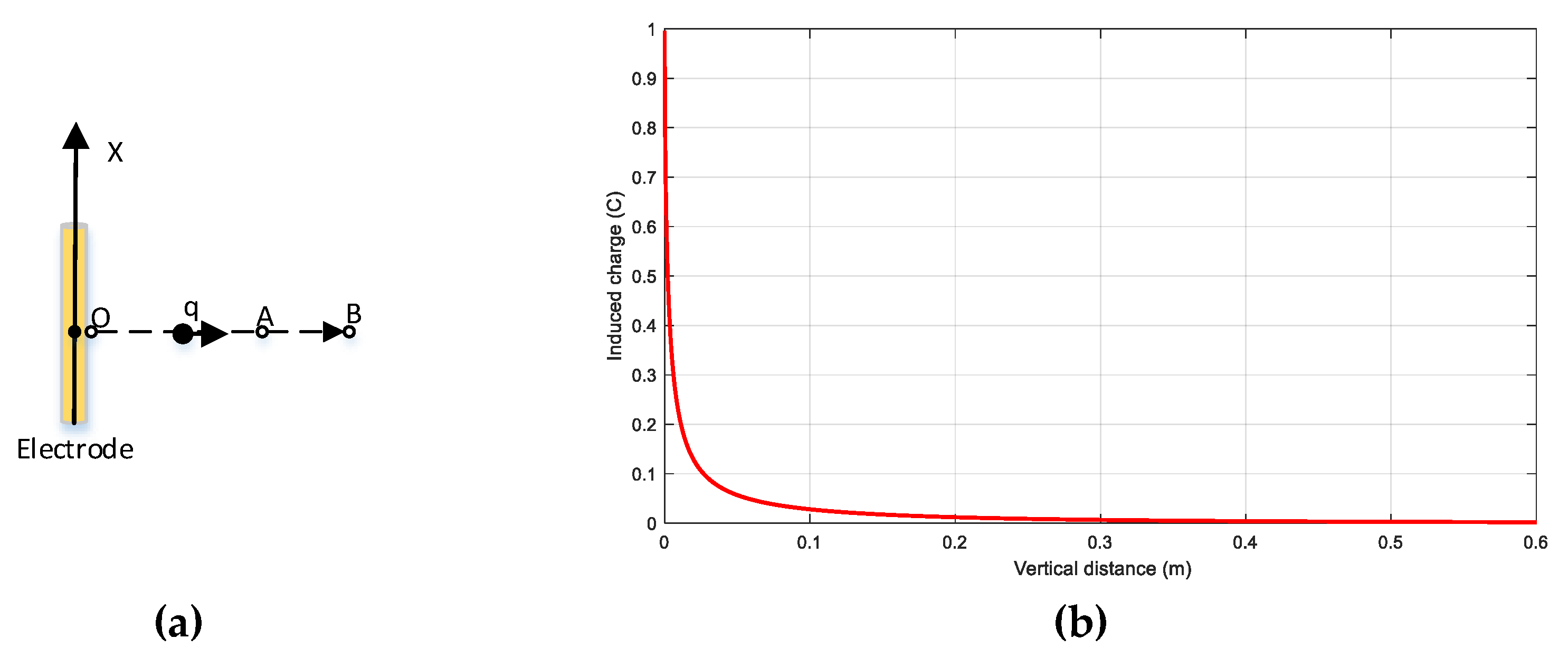
As shown in Figure 7a, the point charge $q$ moves from the surface of the electrode to point $\mathrm{A}$ and then to point $\mathrm{B}$. The distance between point $\mathrm{A}$ and the surface of the electrode is $0.5\mathrm{m}$ and the distance between point $\mathrm{B}$ and the electrode is $0.5\mathrm{m}$, the amount of charge $Q$ is $-1\mathrm{C}$, the radius of rod electrode $r$ is $0.005\mathrm{m}$, and the length of the electrode is $0.5 \mathrm{m}$. As shown in Figure 7b, the closer the point charge is to the electrode, the larger the induced charge. With increased distance from the point charge, the induced charge decreases rapidly. When the distance between the point charge and the electrode reaches a certain value, the change of the induced charge is very small. The trend in Figure 7b can also be observed in Figure 6c. It is also consistent with the conclusion that when the charged particles are evenly distributed around the electrode, the charge on the electrode is induced by a cylindrical region around the electrode with a radius of $0.5\mathrm{m}$.

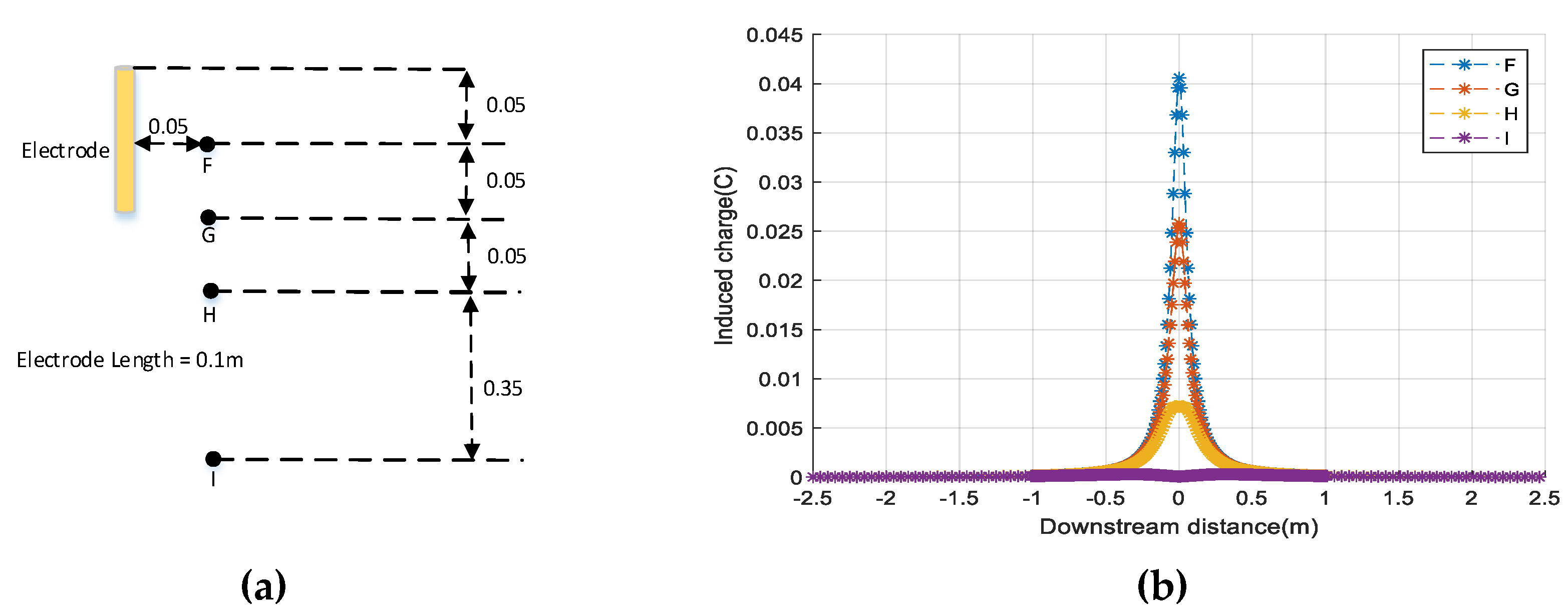
As shown in Figure 8a, the point charge passes through the points $\mathrm{F},\mathrm{G},\mathrm{H},\mathrm{I}$ with a constant velocity v = 5 m/s in a direction perpendicular to the electrode’s axis. The distribution of $\mathrm{F},\mathrm{G},\mathrm{H},\mathrm{I}$ parallel to the length of the electrode is fixed, the amount of the point charge is $Q=-1\mathrm{C}$, the radius of the rod electrode is $r=0.005\mathrm{m}$, and the vertical distance between $\mathrm{F},\mathrm{G},\mathrm{H},\mathrm{I},$ and the surface of the electrode is $h=0.05\mathrm{m}$. The distribution of the induced charge on the electrode is shown in Figure 8b. The amount of the induced charge increases gradually as the point charge gradually approaches the electrode. With the charge point away from the electrode, the amount of the induced charge gradually decreases. The induced charge at point $\mathrm{I}$ is very small, thus it can be concluded that the induced charge by the point charge being farther than $\mathrm{I}$ can be ignored when the charged particles are evenly distributed around the electrode.

The case where the point charge moves in a direction parallel to the axis of the electrode, as shown in Figure 9a, is considered, and the point charge moves from point $\mathrm{A}$ to point $\mathrm{B}$ and then to point $\mathrm{C}$. The distance from point $\mathrm{A}$ to point $\mathrm{C}$ is $1.2 \mathrm{m}$. The charge of the point charge is $Q=-1\mathrm{C}$, the radius of the rod electrode is $r=0.005\mathrm{m}$, and the vertical distance of points $\mathrm{A}$, $\mathrm{B}$, and $\mathrm{C}$ from the surface of the electrode is $h=0.05\mathrm{m}$. The amount of the induced charge is shown in Figure 9b. The amount of the induced charge increases as the length of the electrode increases; the amount of the induced charge on the electrode in the range near the intermediate position of the electrode is larger, and the amount on the electrode becomes smaller. If the point charge is outside the range of the electrode length +0.15 m, the contribution to the amount of the induced charge will be negligible.

From the above analysis, it is concluded that the charged particles capable of inducing a charge on the rod electrode are mostly distributed in the shadow range, as shown in Figure 10. Note that a circular conveying pipe is considered in Figure 10 and the charged particles are uniformly distributed.

3.2.2. Effect of Electrode Length

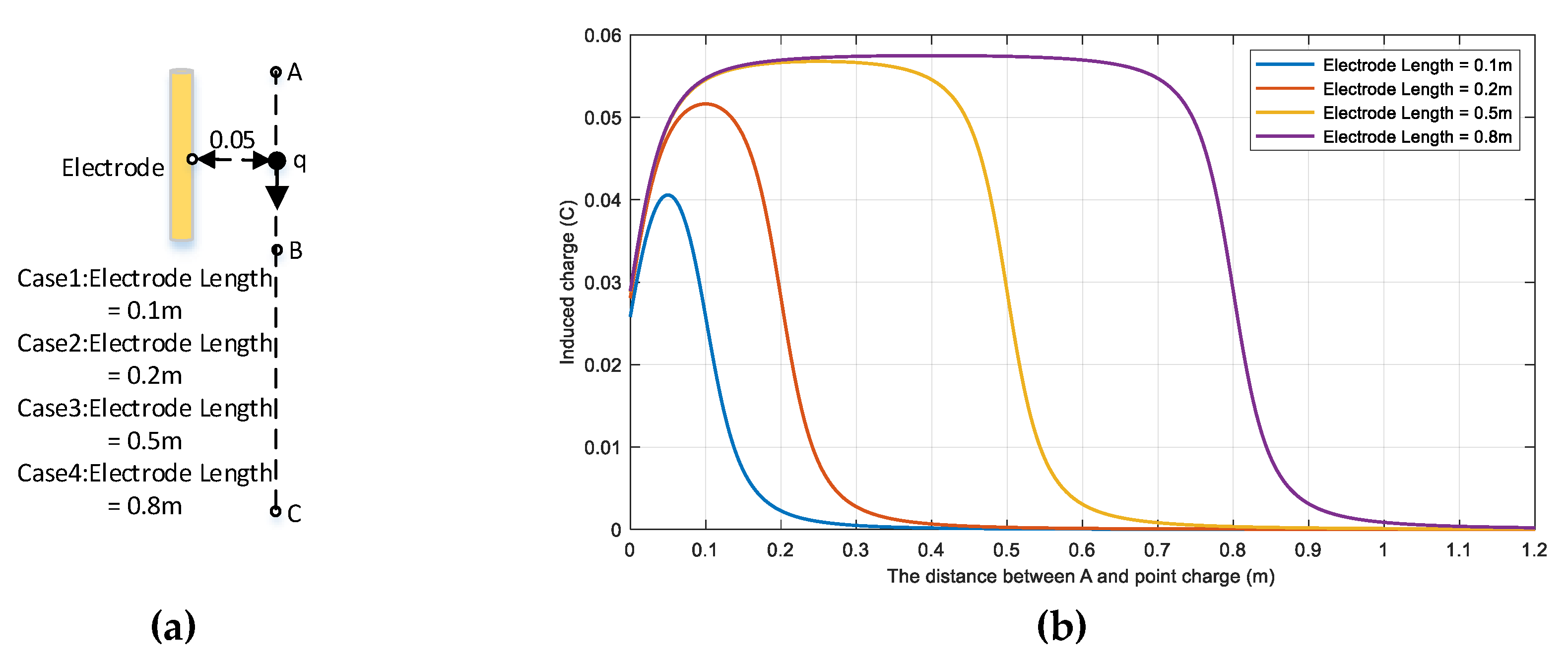
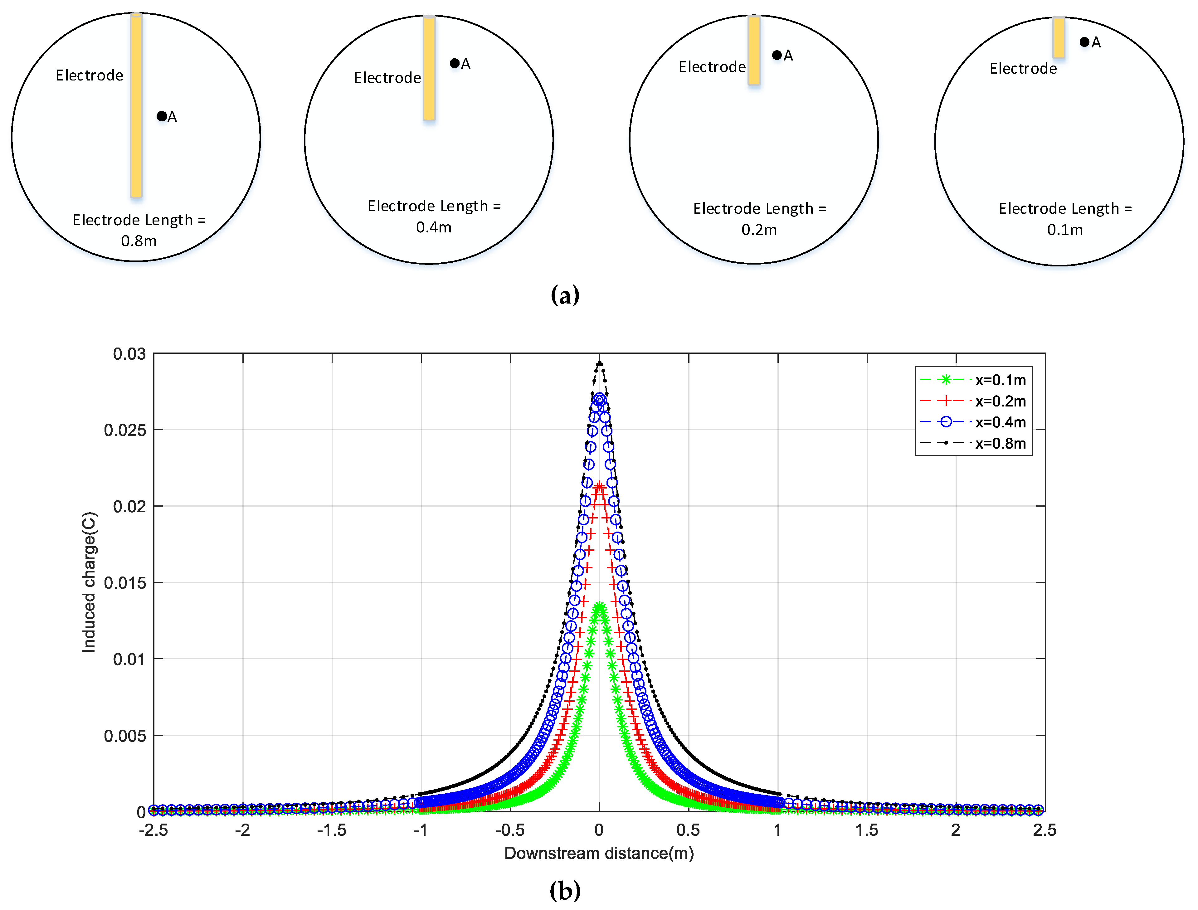
The length of the rod electrode is an important parameter that needs to be determined in the sensor design stage. As shown in Figure 11a, four cases of the electrode length are chosen for the simulation study: $0.8\mathrm{m}$, $0.4\mathrm{m}$, $0.2\mathrm{m}$, and $0.1\mathrm{m}$. The point charge carries charge $Q=-1\mathrm{C}$ and travels with constant velocity $v=5 \mathrm{m}/\mathrm{s}$ passing through point $\mathrm{A}$ in the direction perpendicular to the electrode. The radius of the rod electrode is $r=0.005 \mathrm{m}$, and the distance from point $\mathrm{A}$ to the surface of the electrode is $h=0.05 \mathrm{m}$. The change of the induced charge for the four cases is presented in Figure 11b. It can be observed that as the length of the electrode increases, the amount of the induced charge increases, but the increase rate decreases with the increase of the electrode. It can be concluded that the longer the electrode, the more charge can be induced. However, when the electrode length increases to a certain extent, its growth does not cause a significant change in the amount of the induced charge.

As shown in Figure 12a, the length of the electrode varies from 0 m to 4 m and the distance from the surface of the electrode is $h=0.1\mathrm{m}$. The changed amount of the induced charge on the electrode is shown in Figure 12b. The charge of the point charge is $Q=-1\mathrm{C},$ and the radius of the rod electrode is $r=0.005\mathrm{m}$. As shown in Figure 13b, once the length of the electrode reaches $1\mathrm{m}$ or more, the increase rate of the induced change becomes very small. In other words, increasing the electrode length contributes very little to the amount of the induced charge when the length reaches $1\mathrm{m}$.

3.2.3. Effect of Electrode Radius

As shown in Figure 13a, the distance of four points $\mathrm{J},\mathrm{K},\mathrm{M},\mathrm{and}\mathrm{N}$ from the surface of the electrode is $0.05\mathrm{m}$, $0.10\mathrm{m}$, $0.15\mathrm{m}$, and $0.20\mathrm{m}$, respectively. The charge amount of the point charge is $Q=-1\mathrm{C}$, and the length of the rod electrode is $0.1 \mathrm{m}$. The radius varies from $0.001 \mathrm{m}$ to $0.2\mathrm{m}$. The amount of the induced charge on the electrode is shown in Figure 13b. As the radius of the electrode increases, the amount of the induced charge increases. This means that electrodes with a larger radius can induce more charge, which is beneficial to the design of the detection circuit in later stages. However, the radius of the electrode generally cannot be made too large to adapt to the actual situation in practice.

4. Induced Current on a Rod Electrode by Moving Point Charge

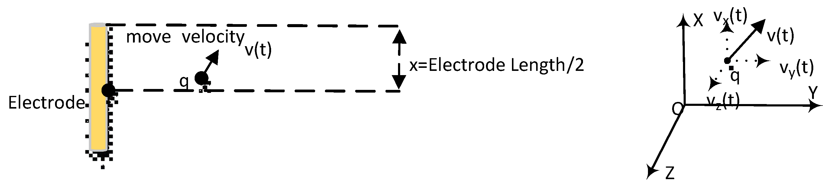
As shown in Figure 14, point charge $q$ moves with velocity $v\left(t\right)$, assuming that its position at time $zero$ is $\left(x_0, y_0, z_0\right)$, then its position at time $t$ is $\left(x_t, y_t, z_t\right)$.

$x_t$, $y_t$, and $z_t$ can be expressed as

$$x_t=x_0+\underset{0}{\overset{t}{{\displaystyle \int }}}{v}_x\left(t\right)dt$$

(15)

$$y_t=y_0+\underset{0}{\overset{t}{{\displaystyle \int }}}{v}_y\left(t\right)dt$$

(16)

$$z_t=z_0+\underset{0}{\overset{t}{{\displaystyle \int }}}{v}_z\left(t\right)dt.$$

(17)

$h$ in Equation (1) can be expressed as

$$h={\left({\left(y_t+r\right)}^2+z_t{}^2\right)}^{1/2}-r.$$

(18)

Equation (13) can be expressed as

$$Q\left(t\right)={{\displaystyle \int }}_{-acos\left(\frac{r}{r+h}\right)}^{acos\left(\frac{r}{r+h}\right)}\left(\frac{-qr{h}^{\prime }\left(x_2-x_t\right)}{2{\pi h}_1{}^2{\left(h_1{}^2+{\left(x_2-x_t\right)}^2\right)}^{\raisebox{1ex}{$1$}\!\left/ \!\raisebox{-1ex}{$2$}\right.}}-\frac{-qr{h}^{\prime }(x_1-x_t)}{2{\pi h}_1{}^2{\left(h_1{}^2+{(x_1-x_t)}^2\right)}^{\raisebox{1ex}{$1$}\!\left/ \!\raisebox{-1ex}{$2$}\right.}}\right)d\theta .$$

(19)

The induced current can be calculated by

$$I\left(t\right)=\frac{dQ\left(t\right)}{dt}.$$

(20)

4.1. Simulation for Induced Current

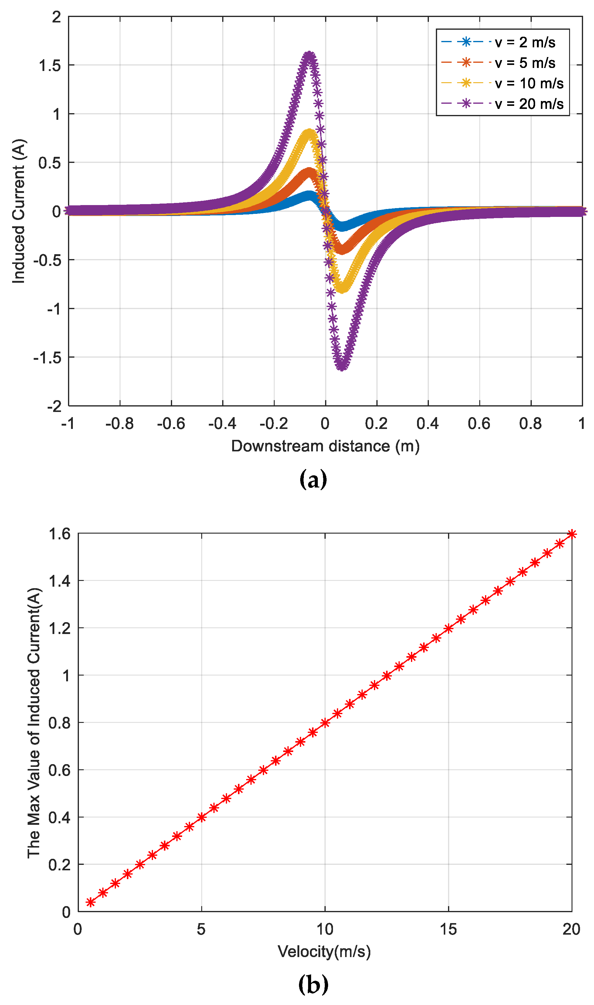
As shown in Figure 14, suppose that point charge $q$ moves from $\left(0, y_0, z_0\right)$ to $\left(0, y_0, -z_0\right)$ with a different constant velocity $v$ of $2\mathrm{m}/\mathrm{s}$, $5\mathrm{m}/\mathrm{s}$, $10\mathrm{m}/\mathrm{s}$, and $20\mathrm{m}/\mathrm{s}$. The charge of the point charge is $Q=-1\mathrm{C}$, $y_0=0.1 \mathrm{m}$, the length of the electrode is $0.1 \mathrm{m}$, and the radius of the electrode is $r=0.005\mathrm{m}$. As shown in Figure 15a, the induced current increases with the increased speed, and the range of the induced current is from $-0.5\mathrm{m}$ to $0.5\mathrm{m}$, which is consistent with the previous analysis in Section 3.2.1.

Figure 15b shows the variation of the maximum induced current with the velocity. Note that the maximum induced current is proportional to the velocity $v_z$ of the point charge.

4.2. Spectrum of Induced Current

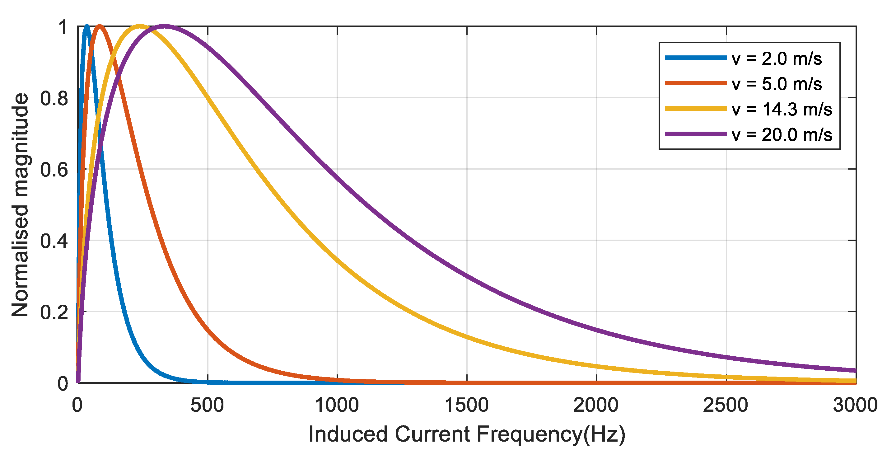
Four velocity cases ($2\mathrm{m}/\mathrm{s}$, 5 $\mathrm{m}/\mathrm{s}$, $14.3\mathrm{m}/\mathrm{s}$, and $20\mathrm{m}/\mathrm{s}$) are selected to study the spectrum of the induced current. As shown in Figure 14, point charge $q$ carries a charge of $-1\mathrm{C}$ and moves from position $\left(0,y_0,z_0\right)$ to position $\left(0,y_0,-z_0\right)$ at velocity $v$, where $z_0=1\mathrm{m}$ and $y_0=0.0015\mathrm{m}$. The length of the electrode is $0.5\mathrm{m}$ and the radius is $r=0.005\mathrm{m}$. The results of the spectrum analysis are shown in Figure 16. It can be seen that the spectrum of the induced current spreads wider as the speed increases. In other words, as the charge moves faster, more abundant frequency components are introduced. This places a requirement on the design of the induced current measurement circuit. In order to capture the signals induced by faster-moving particles, it is necessary to design an acquisition circuit with a sufficiently wide frequency response, which will be discussed in Section 4.4.

4.3. Analysis of the Variation of the Induced Current Spectrum over the Effective Range

To study the variation of the induced current spectrum in the range shown in Figure 10, we take velocity $v=20\mathrm{m}/\mathrm{s}$ as an example. As shown in Figure 14, point charge $q$ moves from $\left(0,y_0,z_0\right)$ to $\left(0, y_0,-z_0\right)$ at constant velocity $v$ parallel to the z-axis direction, where $z_0=1 \mathrm{m}$, the charge of the point charge is $Q=-1\mathrm{C}$, $y_0$ changes from $0.001\mathrm{m}$ to $0.5\mathrm{m}$, the length of the electrode is $0.5\mathrm{m}$, and the radius is $r=0.005\mathrm{m}$. The vertical axis of Figure 17 represents the maximum frequency component. The result indicates that the higher the frequency of the induced current induced by particles closer to the electrode, the lower the frequency of the current induced by particles far from the electrode. In order to acquire high-frequency signals around the electrodes, the detection circuit requires a wide band-pass.

4.4. Measurement Circuit Analysis

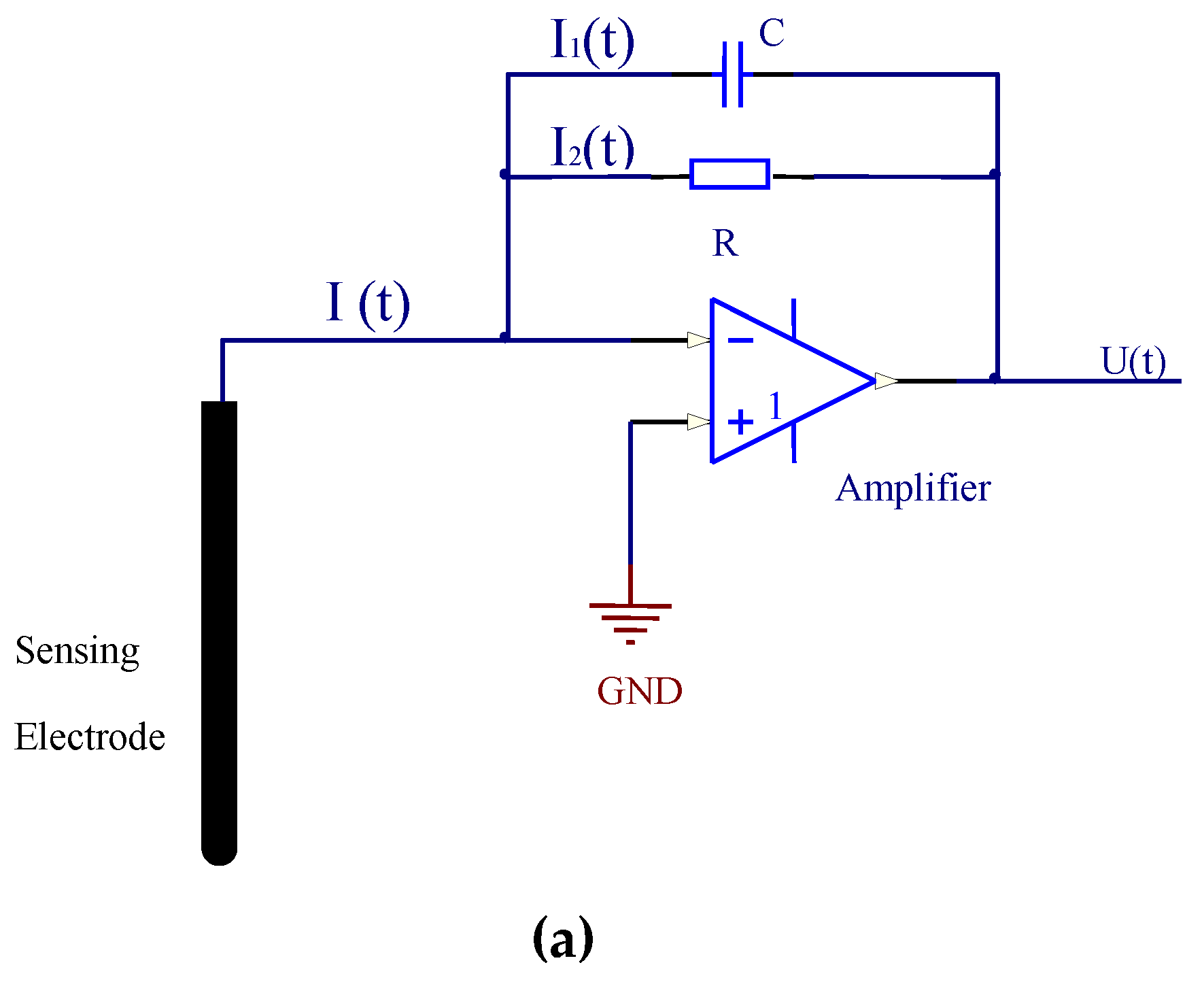
An electrode typically has a high impedance output, hence a charge amplifier is typically added to match the impedance with the input of the data acquisition circuit. A typical charge amplifier is presented in Figure 18a. After passing through the circuit, the induced current signal is converted to a voltage signal. According to the virtual short and virtual break principle of the operational amplifier, it can be obtained that

$$I\left(t\right)=I_1\left(t\right)+I_2\left(t\right)$$

(21)

$$I_1\left(t\right)=-C\frac{dU\left(t\right)}{dt}$$

(22)

$$U\left(t\right)=-I_2\left(t\right)R.$$

(23)

By performing the Fourier transform on Equations (21)–(23), the response of the circuit can be derived as:

$$\frac{U\left(\omega \right)}{I\left(\omega \right)}=-\frac{R}{1+j\omega CR}$$

(24)

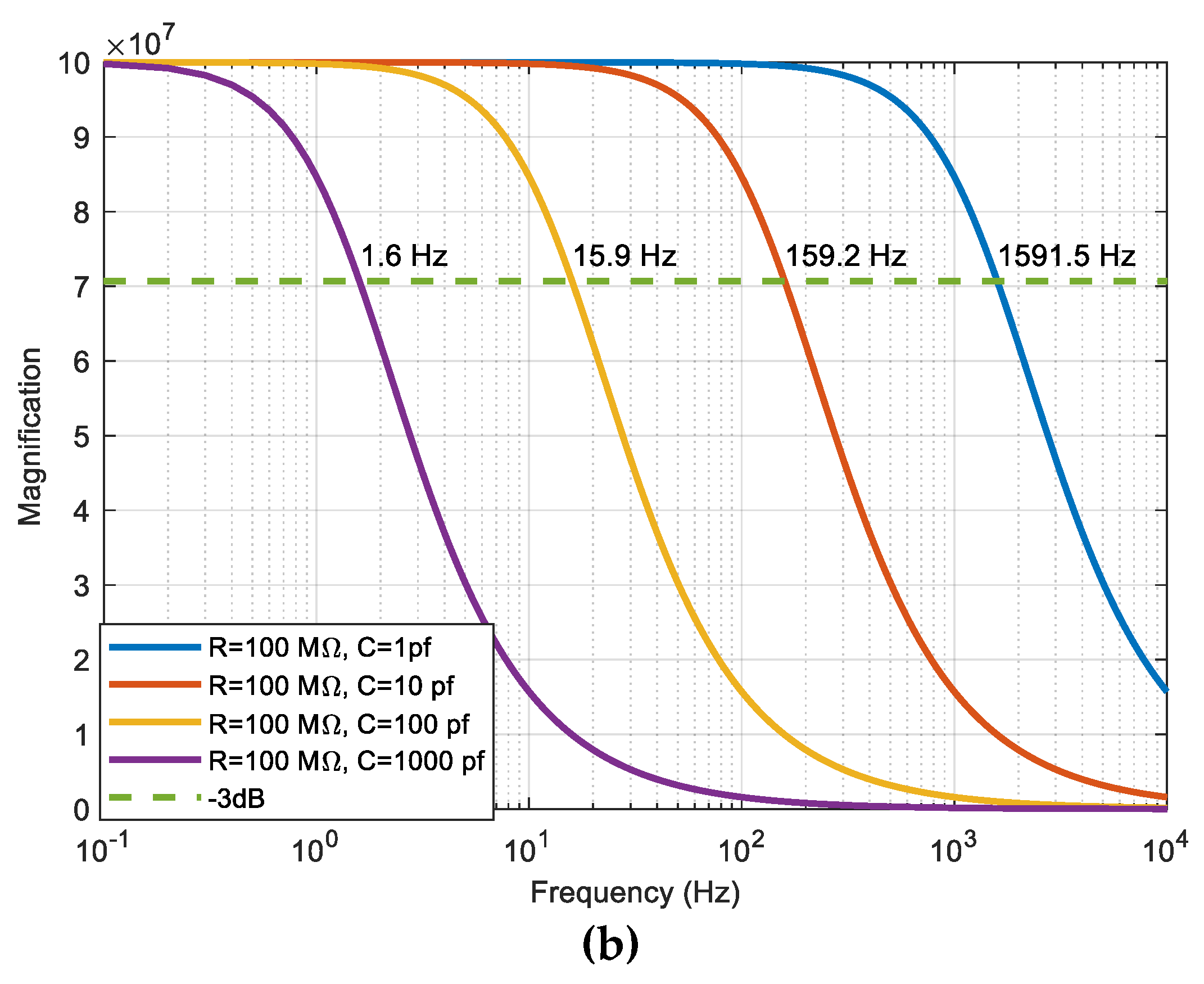
The two most important features of the measurement circuit are its amplification and frequency characteristics. The amplification function is used to amplify the weak induced current signal to the extent that it can be acquired by an analogue to a digital converter. To study the spectral influence of the measurement circuit over the sensing circuit, its frequency characteristics are examined. From Equation (24), it can be concluded that the amplification factor of the output signal is determined by the resistor $R$ and the cutoff frequency of the output signal $U\left(t\right)$ is determined by the capacitor C. The frequency responses by different $R$ and $C$ values are calculated and shown in Figure 18b. It can be observed that the cutoff frequency decreases with the increased $C$.

5. Experimental Study and Discussion

From the simulation study in Section 4, we can understand the signals of the induced current by a moving point charge. In this section, an experimental system is set up and three experiments are performed to validate the established model.

5.1. Experimental Setup

The schematic of the experimental system is shown in Figure 19a. A rod electrode is placed on a supporting holder parallel to the ground, and a funnel is placed on top of the electrode. During the experiment, a charged ball is released from the funnel toward the ground. By adjusting the distance Height1 between supporting rods 1 and 2, the moving speed of the charged ball can be adjusted. The distance Height2 between supporting rod 2 and the ground can decide the final speed of the charging ball. Note that supporting rod 2 is made of insulating material to hold the rod electrode. In addition, supporting rods 1 and 2 are adjustable to a full 360°, hence the horizontal distance between the small ball and the rod electrode can be adjusted by changing the angle between supporting rods 1 and 2; that is, parameter $h$ in Equation (19).

A picture of the rod electrode employed in this paper is shown in Figure 19b. The rod electrode is made of a 316L stainless steel, with a radius of 0.005 m and a length of 0.5 m. Note that the surface is coated with a Teflon insulation 0.3 mm thick to ensure that the current on the electrode is entirely induced by the electrostatic induction.

The output of the rod electrode was connected to a charge amplifier for amplification, as shown in Figure 18a, with $R=100\mathrm{M}\mathrm{\Omega }$ and $C=10\mathrm{pf}$. According to the analysis in Section 4.4, the cutoff frequency was set at 159.2 Hz with such a setting. In the experiment, the maximum moving speed of the ball was less than 6 m/s, so the signal of interest could be appropriately magnified based on the analysis in Figure 16. Then, the signal was acquired by a data acquisition board and sent to the computer for further analysis. From the analysis in Section 4, we understand that the highest frequency of the signal is below 3500 Hz, so the sampling rate of the data acquisition board was set at 10 kHz to satisfy the Nyquist sampling theorem, i.e., the sampling frequency should be more than twice the maximum frequency.

The experiments are conducted in an environment with room temperature (about 20–25 °C) and normal pressure (about 101 kPa).

5.2. Results and Discussion

Three situations were analyzed in this study, and in all these experiments, the gravity acceleration $g$ was assumed to be $9.8 \mathrm{m}/{\mathrm{s}}^2$ and the ball fell from the funnel at an initial velocity of 0 m/s, hence the velocity of the ball at time $t$ can be calculated by $v\left(t\right)=gt$.

Experiment 1: $Height1=0.57 \mathrm{m}$, $Height2=0.90\mathrm{m}$, $h=0.33\mathrm{m}$, ball carries a charge of $q=486 \mathrm{nC}$ $v\left(t\right)=gt$. Hence, the velocity of the ball reached $3.34 \mathrm{m}/\mathrm{s}$ when passing by the rod electrode and reached $5.37 \mathrm{m}/\mathrm{s}$ when it landed on the ground. The measured signal by the rod electrode and its spectrum are shown in Figure 20a,b, respectively. As can be observed, there exists a DC component in the measured signal in Figure 20a. This DC component is from the data acquisition board, not from the true signal, as the data acquisition board has an added offset of 2.5 V to the input signal, converting the input voltage of −2.5 V to 2.5 V to 0 to 5 V. Hence, this DC component should be removed before further processing. It can be observed that the signal interfered with a severe 50 Hz power line signal and the signal of interest mainly falls within 20 Hz. With a proper low-pass digital filter, the power line frequency can easily be removed. The filtered signal and its spectrum are presented in Figure 20c,d, respectively. In Figure 20c, the voltage increases at the beginning when the ball moves nearer to the rod electrode, indicating that the rate of increase of the induced charge is increasing. Then, the voltage decreases to zero, indicating that the rate of increase of the induced charge is decreasing, and the induced charge reaches the maximum value when the ball is nearest to the electrode, at which point the voltage output is equal to zero.

As the ball moves away from the electrode, the voltage becomes negative, indicating that the induced charge on the electrode becomes smaller. The smaller the voltage, the larger the loss rate. When the loss rate becomes the smallest, then it becomes larger, indicating that the loss rate of the induced charge becomes smaller. At the point where the voltage reaches zero again, the induced charge returns to zero. This is in agreement with the fact that when a charged ball moves to an electrode, the electrode will induce charges, and the induced charges will be reduced when the charged ball moves away from the electrode.

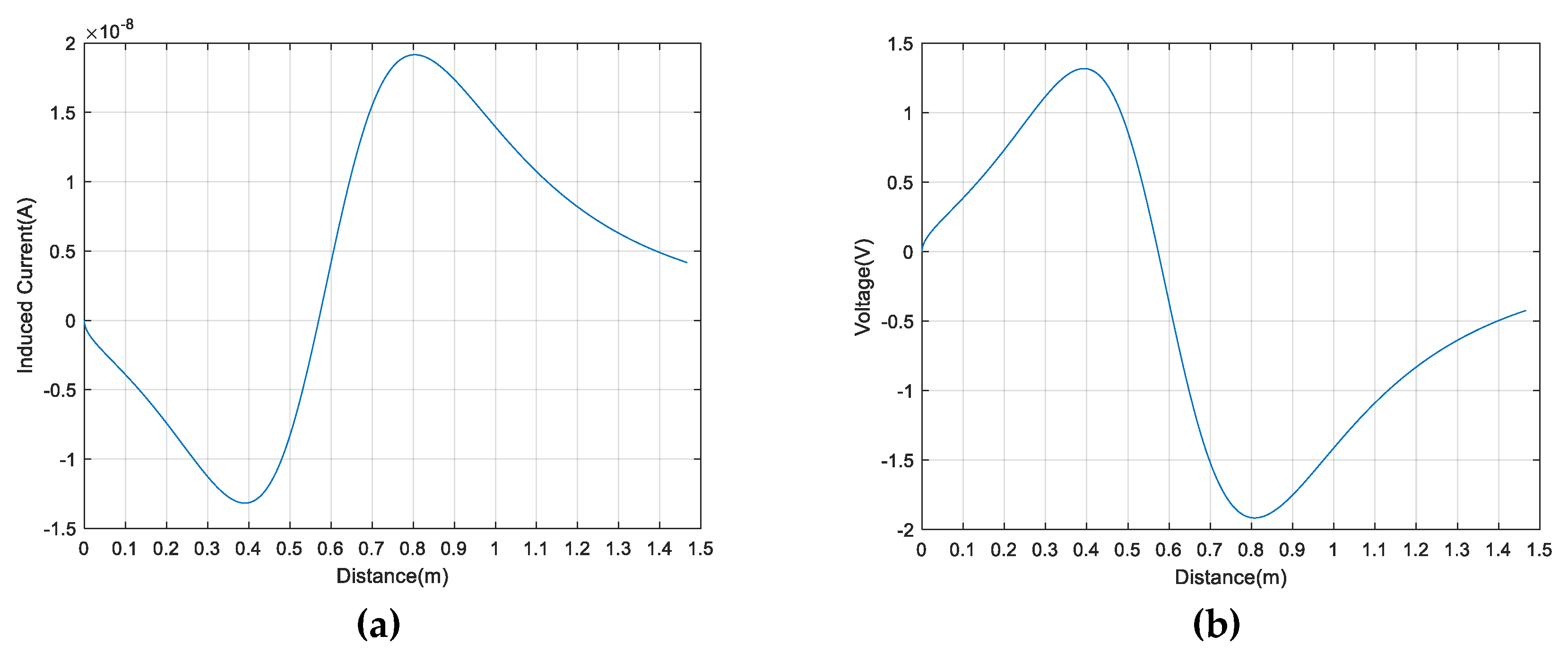
By using Equation (19), the induced current change with the distance between the ball and the funnel is calculated and presented in Figure 21a. The simulated signal output after the charge amplifier is shown in Figure 21b. It can be observed that this signal shows good similarity with the experimental output signal (Figure 20c) in both the shape and amplitude. The induced current increases to a maximum value with the ball moving close to the electrode, and then decreases to zero when the ball is closest to the electrode, corresponding with Figure 15a. The validity of the model is verified.

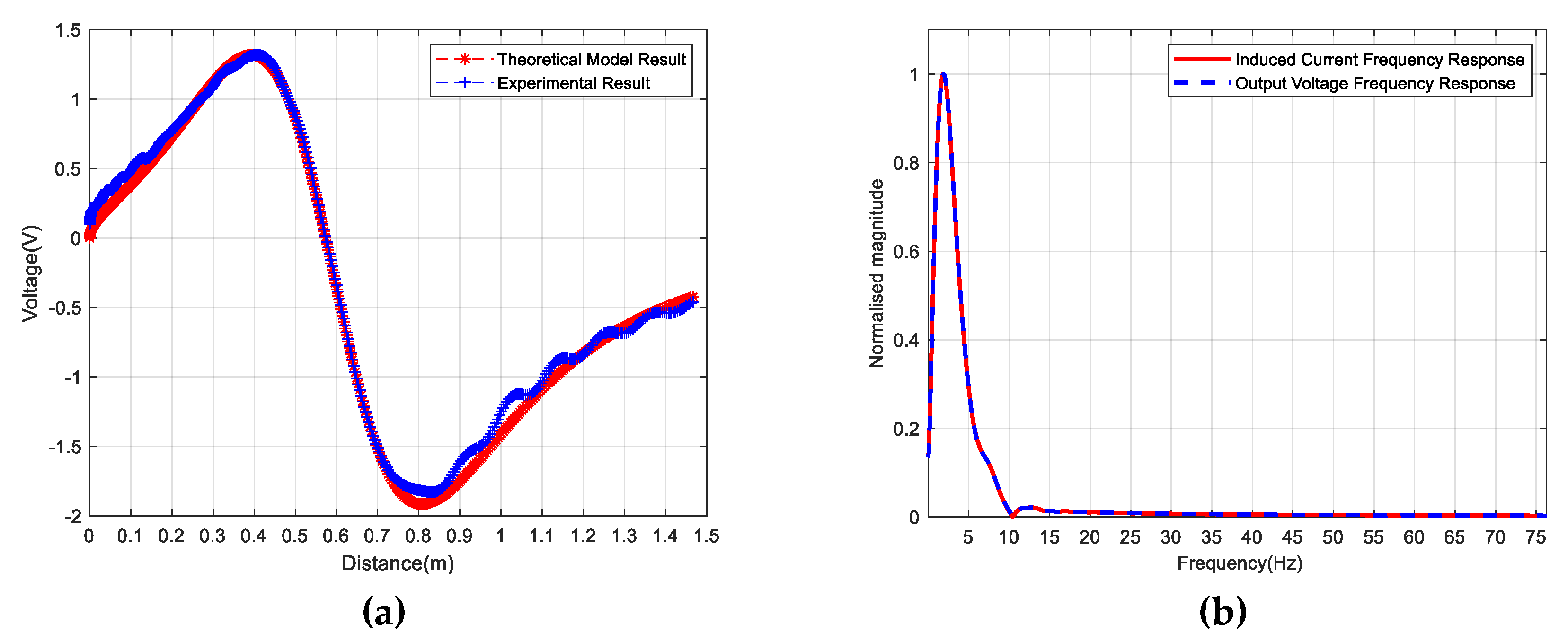
By resetting the time when the ball leaves the funnel at zero and converting the time to distance in Figure 20c, the theoretical output and measured signal are plotted together in Figure 22a and their spectra are compared in Figure 22b. It shows that these two signals have a high similarity in trend and their values are very close to each other, verifying the correctness of the model we established. Specifically, when the charged ball moved with a low velocity (distance Height 1 is less than 0.8 m or velocity is less than 4 m/s), the theoretical and measured waveforms agreed very well. When the charged ball moved with a high velocity, i.e., velocity greater than 4 m/s, the measured signal was smaller than the theoretical one. A possible reason for this phenomenon could be that the charged ball experiences more resistance from the air with the increased velocity, which reduces the velocity of the ball to a level lower than theoretical calculations and hence less current is induced on the rod electrode.

Experiment 2: $Height1=0.80 \mathrm{m}$, $Height2=0.90 \mathrm{m}$, $h=0.17 \mathrm{m}$, ball 1 carried a charge of $37.13 \mathrm{nC}$ and ball 2 carried a charge of $57.22 n\mathrm{C}$. Hence, the velocity of the ball reached $3.96 \mathrm{m}/\mathrm{s}$ when it passed by the rod electrode and reached $5.72 \mathrm{m}/\mathrm{s}$ when it landed on the ground.

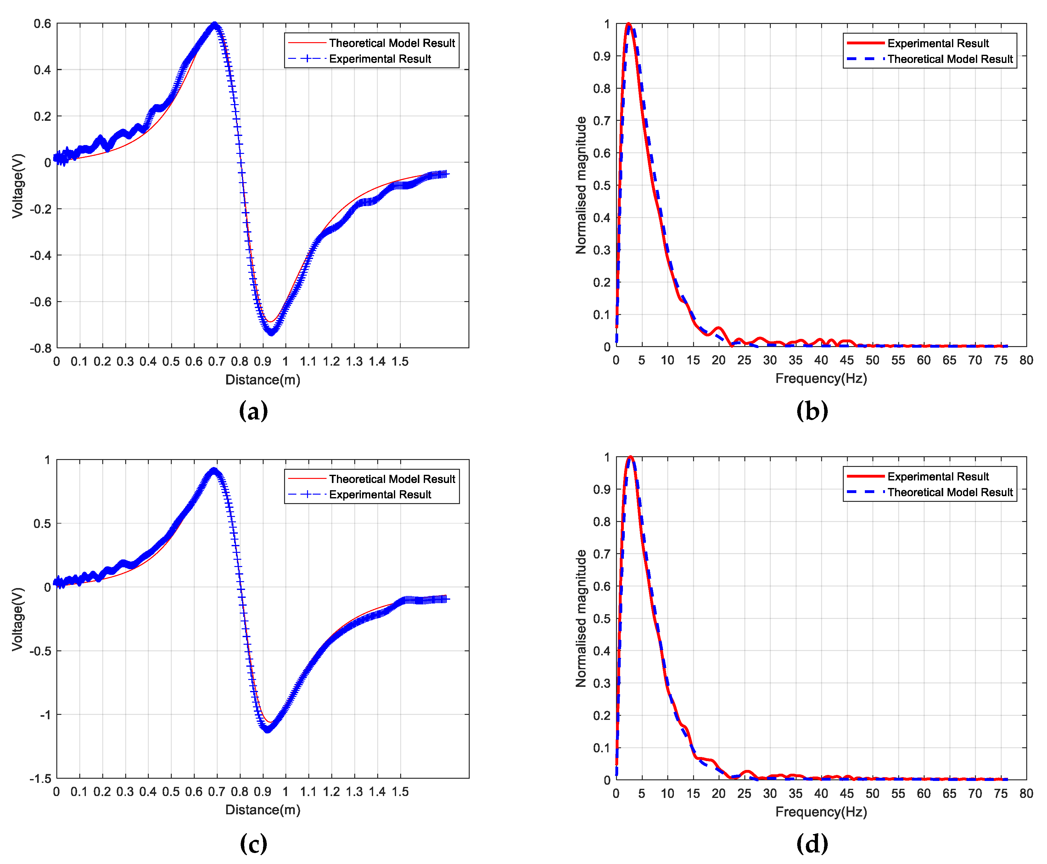
The theoretical and measured output voltages are shown in Figure 23a. As can be observed, the waveforms show similar trends as those in Experiment 1. The induced current increased accordingly with the increased velocity of the ball, which is reflected by the maximum and minimum amplitude of the induced current. By comparing Figure 23a,c, it can be seen that the induced voltage increased significantly, mainly caused by an increased charge carried by the ball. This can be explained by Equation (19), which shows that the induced current is proportional to the amount of charge if other conditions remain unchanged. Taking the maximum value, minimum value, and measured value at four similar distances in Figure 23a,c, the results are summarized in

Table 1. Comparison of the experimental results between charged ball 1 and charged ball 2.

	Charged Ball 1	Charged Ball 2	Ratio
Amount of charge (nC)	37.13	57.22	0.6490
Maximum measured value (V)	0.5909	0.9107	0.6488
Minimum measured value (V)	−0.7333	−1.1190	0.6553
Measured value at 0.5 m (V)	0.2788	0.4299	0.6485
Measured value at 0.6 m (V)	0.4794	0.6864	0.6984
Measured value at 1.1 m (V)	−0.4138	−0.6335	0.6531
Measured value at 1.2 m (V)	−0.2881	−0.4112	0.7006

. It can be observed that the induced current is approximately proportional to the amount of charge.

Experiment 3: $Height1=0.45 \mathrm{m}$, $Height2=0.90 \mathrm{m}$, $h=0.18 \mathrm{m}$, ball carried a charge of $134 \mathrm{nC}$. Hence, the velocity of the ball reached $2.97 \mathrm{m}/\mathrm{s}$ when it passed by the electrode and reached $5.14 \mathrm{m}/\mathrm{s}$ when it landed on the ground.

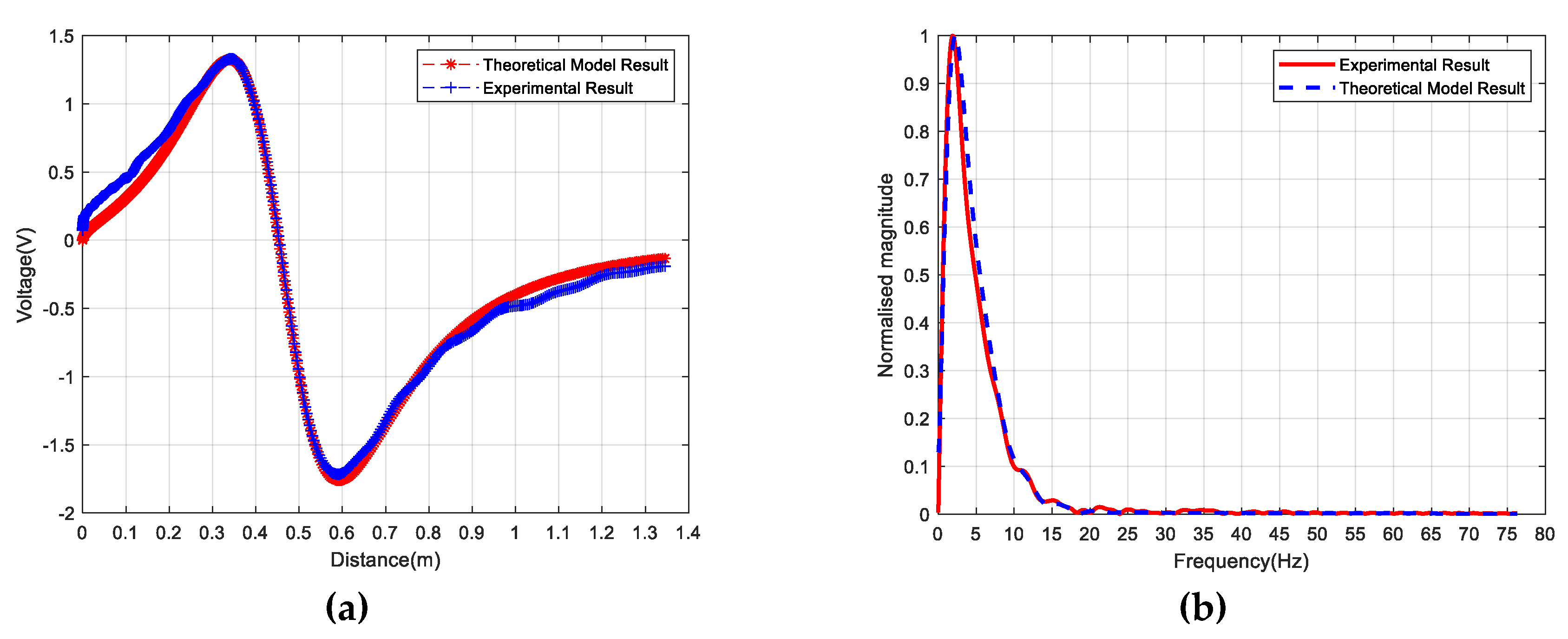
The comparison of the output voltage between the theoretical and experimental waveforms is shown in Figure 24a and the spectrum comparison is shown in Figure 24b. By comparing Figure 22a and Figure 24b, it can be seen that the high-frequency component decreases when $h$ increases, which is consistent with the analysis in Section 4.3.

Through three experiments with different scenario settings, it can be observed that the established model matches well with the experimental measurements, verifying the correctness and accuracy of the model. In addition, the following observations are also verified:

(1)

The induced current decreased significantly with the increase of $h$, which can be observed in Figure 22b and Figure 24a, and this is in line with the result in Figure 7b.

(2)

The high-frequency components of the induced current are reduced with the increased $h$, which can be seen by comparing Figure 22a and Figure 24b, and this is consistent with Figure 17.

(3)

The high-frequency components increase with the increased velocity, which can be observed by comparing Figure 23b and Figure 24b.

(4)

When the velocity and the $h$ value are fixed, the change in the amount of the charge on the ball does not influence the spectral characteristics of the induced current signal, which can be observed in Figure 23b,d.

6. Conclusions

In this paper, a theoretical model of the induced charge on a rod electrode by a point charge is established by the method of images and the accuracy of the model is verified by three experimental studies. The following conclusions are drawn based on the study.

• The amount of the induced charge on the rod electrode are mainly determined by the following factors: The distance between the point charge and the electrode, the radius and the length of the electrode.
• The general model of the relationship between the induced current and velocity is established and the spectrum of the induced current is studied. The induced current increases with the increase of the point charge’s velocity and the maximum value of the induced current is linearly proportional to the point charge’s velocity. The faster the velocity of the point charge, the wider the spectrum of the induced current. The further the point charge from the rod electrode, the narrower the spectrum of the induced current on the rod electrode.
• For the measurement circuit, its amplification ratio and pass-band width are determined by the feedback resistance and feedback capacitance, respectively. With the increase of the feedback resistance, the amplification factor of the circuit increases. With the increase of the feedback capacitance, the pass-band width of the measurement circuit becomes narrower.

The phenomena observed in the experiments, which are well explained by the established model, would be not so easy to explain with just the qualitative analysis. This model provides a basis for more complex studies in the future; for example, the sum result of all the particles around the electrode can been studied with this model. In addition, the influence of the length and radius of the rod electrode on the induced charge are also studied, providing theoretical support for the rod electrode sensor development in the future.

References

- Lebecki, K.; Małachowski, M.; Sołtysiak, T. Continuous dust monitoring in headings in underground coal mines. J. Sustain. Min. 2016, 15, 125–132. [Google Scholar] [CrossRef]
- Brodny, J.; Tutak, M. Exposure to Harmful Dusts on Fully Powered Longwall Coal Mines in Poland. Int. J. Environ. Res. Public Health 2018, 15, 1846. [Google Scholar] [CrossRef] [PubMed]
- Jeong, W.; Jeon, S.; Jeong, D. Advanced Backstepping Trajectory Control for Skid-Steered Duct-Cleaning Mobile Platforms. Electronics 2019, 8, 401. [Google Scholar] [CrossRef]
- Mataloto, B.; Ferreira, J.C.; Cruz, N. LoBEMS—IoT for Building and Energy Management Systems. Electronics 2019, 8, 763. [Google Scholar] [CrossRef]
- Marques, G.; Pitarma, R. A Cost-Effective Air Quality Supervision Solution for Enhanced Living Environments through the Internet of Things. Electronics 2019, 8, 170. [Google Scholar] [CrossRef]
- Arroyo, P.; Lozano, J.; Suárez, J.I. Evolution of Wireless Sensor Network for Air Quality Measurements. Electronics 2018, 7, 342. [Google Scholar] [CrossRef]
- Gajewski, J. Electrostatic Nonintrusive Method for Measuring the Electric Charge, Mass Flow Rate, and Velocity of Particulates in the Two-Phase Gas–Solid Pipe Flows—Its Only or as Many as 50 Years of Historical Evolution. IEEE Trans. Ind. Appl. 2008, 44, 1418–1430. [Google Scholar] [CrossRef]
- Weinheimer, A.J. The charge induced on a conducting cylinder by a point charge and its application to the measurement of charge on precipitation. J. Atmos. Ocean. Technol. 1988, 5, 298–304. [Google Scholar] [CrossRef]
- Woodhead, S.R.; Amadi-Echendu, J.E. Solid phase velocity measurement utilizing electrostatic sensors and cross correlation signal processing. In Proceedings of the 1995 IEEE Instrumentation and Measurement Technology Conference, Waltham, MA, USA, 23–26 April 1995; pp. 774–777. [Google Scholar]
- Gajewski, J.B. Non-contact electrostatic flow probes for measuring the flow rate and charge in the two-phase gas–solids flows. Chem. Eng. Sci. 2006, 61, 2262–2270. [Google Scholar] [CrossRef]
- Yan, Y.; Byrne, B.; Woodhead, S.; Coulthard, J. Velocity measurement of pneumatically conveyed solids using electrodynamic sensors. Meas. Sci. Technol. 1995, 6, 515–537. [Google Scholar] [CrossRef]
- Qian, X.; Yan, Y.; Huang, X.; Hu, Y. Measurement of the Mass Flow and Velocity Distributions of Pulverized Fuel in Primary Air Pipes Using Electrostatic Sensing Techniques. IEEE Trans. Instrum. Meas. 2017, 66, 944–952. [Google Scholar] [CrossRef]
- Li, L.; Hu, H.; Qin, Y.; Tang, K. Digital Approach to Rotational Speed Measurement Using an Electrostatic Sensor. Sensors 2019, 19, 2540. [Google Scholar] [CrossRef] [PubMed]
- Xu, C.; Wang, S.; Tang, G.; Yang, D.; Zhou, B. Sensing characteristics of electrostatic inductive sensor for flow parameters measurement of pneumatically conveyed particles. J. Electrost. 2007, 65, 582–592. [Google Scholar] [CrossRef]
- Li, J.; Ma, X.; Zhao, M.; Cheng, X. A Novel MFDFA Algorithm and Its Application to Analysis of Harmonic Multifractal Features. Electronics 2019, 8, 209. [Google Scholar] [CrossRef]
- S´wirad, S.; Wydrzynski, D.; Nieslony, P.; Krolczyk, G.M. Influence of hydrostatic burnishing strategy on the surface topography of martensitic steel. Measurement 2019, 138, 590–601. [Google Scholar] [CrossRef]
- Osornio-Rios, R.A.; Antonino-Daviu, J.A.; Romero-Troncoso, R.d.J. Recent Industrial Applications of Infrared Thermography: A Review. IEEE Trans. Ind. Inf. 2019, 15, 615–625. [Google Scholar] [CrossRef]
- Mia, M.; Królczyk, G.; Maruda, R.; Wojciechowski, S. Intelligent Optimization of Hard-Turning Parameters Using Evolutionary Algorithms for Smart Manufacturing. Materials 2019, 12, 879. [Google Scholar] [CrossRef] [PubMed]
- Glowacz, A. Fault Detection of Electric Impact Drills and Coffee Grinders Using Acoustic Signals. Sensors 2019, 19, 269. [Google Scholar] [CrossRef]
- Wang, C.; Zhan, N.; Jia, L.; Zhang, J.; Li, Y. DWT-based adaptive decomposition method of electrostatic signal for dilute phase gas-solid two-phase flow measuring. Powder Technol. 2018, 329, 199–206. [Google Scholar] [CrossRef]
- Zhang, W.; Cheng, X.; Hu, Y.; Yan, Y. Measurement of moisture content in a fluidized bed dryer using an electrostatic sensor array. Powder Technol. 2018, 325, 49–57. [Google Scholar] [CrossRef]
- Yang, Y.; Zhang, Q.; Zi, C.; Huang, Z.; Zhang, W.; Liao, Z.; Wang, J.; Yang, Y.; Yan, Y.; Han, G. Monitoring of particle motions in gas-solid fluidized beds by electrostatic sensors. Powder Technol. 2017, 308, 461–471. [Google Scholar] [CrossRef] [Green Version]
- Dong, K.; Zhang, Q.; Huang, Z.; Liao, Z.; Wang, J.; Yang, Y. Experimental investigation of electrostatic effect on bubble behaviors in gas-solid fluidized bed. AIChE J. 2015, 61, 1160–1171. [Google Scholar] [CrossRef]
- Qian, X.; Yan, Y.; Wang, L.; Shao, J. An integrated multi-channel electrostatic sensing and digital imaging system for the on-line measurement of biomass–coal particles in fuel injection pipelines. Fuel 2015, 151, 2–10. [Google Scholar] [CrossRef]
- Liu, S.; Chen, Q.; Wang, H.G.; Jiang, F.; Ismail, I.; Yang, W.Q. Electrical capacitance tomography for gas–solids flow measurement for circulating fluidized beds. Flow Meas. Instrum. 2005, 16, 135–144. [Google Scholar]
- Yao, J.; Zhao, Y.L.; Fairweather, M. Numerical simulation of turbulent flow through a straight square duct. Appl. Therm. Eng. 2015, 91, 800–811. [Google Scholar] [CrossRef]
- Zhang, S.; Yan, Y.; Qian, X.; Hu, Y. Mathematical Modeling and Experimental Evaluation of Electrostatic Sensor Arrays for the Flow Measurement of Fine Particles in a Square-Shaped Pipe. IEEE Sens. J. 2016, 16, 8531–8541. [Google Scholar]
- Wang, L.; Yan, Y.; Hu, Y.; Qian, X. Rotational Speed Measurement Using Single and Dual Electrostatic Sensors. IEEE Sens. J. 2015, 15, 1784–1793. [Google Scholar]
- Coombes, J.R.; Yan, Y. Experimental investigations into the flow characteristics of pneumatically conveyed biomass particles using an electrostatic sensor array. Fuel 2015, 151, 11–20. [Google Scholar] [CrossRef]
- Krabicka, J.; Yan, Y. Finite-Element Modeling of Electrostatic Sensors for the Flow Measurement of Particles in Pneumatic Pipelines. IEEE Trans. Instrum. Meas. 2009, 58, 2730–2736. [Google Scholar] [CrossRef]
- Shao, J.; Krabicka, J.; Yan, Y. Velocity Measurement of Pneumatically Conveyed Particles Using Intrusive Electrostatic Sensors. IEEE Trans. Instrum. Meas. 2010, 59, 1477–1484. [Google Scholar] [CrossRef]
- Shao, J.; Krabicka, J.; Yan, Y. Comparative study of electrostatic sensors with circular and probe electrodes for velocity measurement of pulverized coal. IEEE Trans. Instrum. Meas. 2010, 59, 1477–1484. [Google Scholar]
- Chen, J.-G.; Wu, F.-X.; Wang, J. Dust concentration detection technology of charge induction method. J. Chin. Coal Soc. 2015, 40, 713–718. [Google Scholar]
- Griffiths, D.J. Introduction to Electrodynamics, 4th ed.; Addison-Wesley: Reading, MA, USA, 2012; pp. 124–126. [Google Scholar]
Figure 1.
Working principle figure of the electrode and its application: (a) Schematic figure; (b) in the iron mining company; (c) in the laboratory; and (d) in the steel mill company figure.
Figure 2.
Steps of the proposed method to model the induced charge on a rode electrode.
Figure 3.
Rod electrode induced charge model: (a) Point charge q and its image; (b) electric field line distribution; (c) coordinate system; (d) projection of point on plane ; (e) calculation of the field strength of B using the image method; and (f) determining the range of .
Figure 4.
Induced charge density along θ: (a) Illustration of the point charge position, and (b) induced charge density.
Figure 5.
Distribution of the induced charge along .
Figure 6.
Locations of point charges A, B, C, D, E in the pipeline: (a) Point charge moving in the pipeline; (b) point charge distance from the electrode; and (c) induced charge of the point charge moving perpendicular to the electrode’s axis.
Figure 7.
Point charge away from the electrode: (a) Charge moving perpendicular to the electrode; and (b) induced charge change.
Figure 8.
Locations of point charges F, G, H, I in the pipeline: (a) Position of the point charge and electrode; and (b) amount of the induced charge on the electrode as distance changes.
Figure 9.
The point charge moves in a direction parallel to the axis of the electrode: (a) State of moving the point charge parallel to the electrode; and (b) amount of charge induced by moving the point charge parallel to the electrode.
Figure 10.
Active induced range of the rod electrode.
Figure 11.
(a) Electrodes of different lengths and positions of the point charge; (b) induced charge distribution on electrodes of different lengths.
Figure 12.
Effect of the electrode length change on the induced charge: (a) Increasing the length of the sensing electrode; and (b) variation of the amount of the induced charge with the electrode length.
Figure 13.
Effect of the electrode radius: (a) Positions of different point charges and (b) variation of the induced charge with the electrode radius under the influence of the point charge at different positions.
Figure 14.
Moving point charge model.
Figure 15.
(a) Induced current under the effect of the point charge moving at different velocities, and (b) variation of the maximum induced current with the velocity change.
Figure 16.
Spectrum analysis of the induced current under different moving speeds.
Figure 17.
Variation of the main frequency and point charge position of the induced current spectrum under the action of the point charge moving at 20 m/s.
Figure 18.
(a) Schematic of the measurement circuit, and (b) amplitude response of the circuit under different parameter settings.
Figure 19.
Experimental setup: (a) Schematic of the experimental system; (b) picture of the rod electrode employed; and (c) schematic of the signal connection.
Figure 20.
Results of experiment 1: (a) Measurement signal waveform; (b) spectrum of the measurement signal waveform; (c) filtered signal; and (d) spectrum of the filtered signal.
Figure 21.
(a) Theoretical induced current, and (b) theoretical output after the charge amplifier.
Figure 22.
Comparison of the theoretical and measured signal comparison: (a) Time domain waveform, and (b) spectrum.
Figure 23.
Results of experiment 2: (a) Comparison of the theoretical value with the measured voltage of charged ball 1; (b) comparison of the theoretical spectrum with the measured voltage spectrum of charged ball 1; (c) comparison of the theoretical value with the measured voltage of charged ball 2; and (d) comparison of the theoretical spectrum with the measured voltage spectrum of charged ball 2.
Figure 24.
Results of experiment 3: (a) Comparison of the theoretical value with the measured voltage; and (b) comparison of theoretical spectrum with the measured spectrum of voltage.