Specific Emitter Identification Using IMF-DNA with a Joint Feature Selection Algorithm


1
School of Electronics and Information Engineering, Harbin Institute of Technology, Harbin 150001, China
2
College of Computer Science and Information Technology, University of Bahri, Khartoum 12217, Sudan
*
Author to whom correspondence should be addressed.
Electronics 2019, 8(9), 934; https://doi.org/10.3390/electronics8090934
Submission received: 24 July 2019
/
Revised: 22 August 2019
/
Accepted: 23 August 2019
/
Published: 25 August 2019
(This article belongs to the Section Circuit and Signal Processing)
Abstract
:Specific emitter identification (SEI) is a technique to distinguish among different emitters of the same type using weak individual characteristics instead of conventional modulation parameters. The biggest challenge in SEI is to not only distinguish the different emitters with close modulation parameters but also to identify a specific emitter when its modulation parameters change significantly. For this paper, individual differences in pulse envelopes were investigated and four types of pulse envelopes were modeled. To exploit the individual features along with the pulse envelope for the identification of a specific emitter, an intrinsic mode function distinct native attribute (IMF-DNA) feature extraction algorithm and a joint feature selection (JFS) algorithm were proposed, which together constitute the final proposed SEI technique. Compared with four other feature selection methods, the proposed feature selection algorithm performed better for finding the most useful features for classification, which greatly helps in the reduction of feature dimension. Compared with radio frequency DNA (RF-DNA), IMF-DNA had a far superior correct emitter identification rate under similar conditions. A real data verification method was developed to verify the performance of IMF-DNA for specific emitter identification. The method achieved a correct identification rate of 85.3% at a sampling rate of 200 MHz and had an estimated signal-to-noise ratio (SNR) of approximately 10 dB.
1. Introduction
Specific emitter identification (SEI) is a widely applied practical technique for electromagnetic environmental perception, both in modern electronic warfare and many civilian scenarios [1,2]. In modern electronic warfare, radar emitter recognition (RER), which is an important research area of electronic reconnaissance, has faced some challenges in recent years, such as the intentional and random variation of modulation parameters [3,4,5]. SEI was proposed to solve these problems. However, it is difficult to ensure the valid and reliable performance of SEI if only some conventional characteristic parameters are extracted and used for SEI. There is an urgent need for new features that can indicate individual minor differences between different devices of the same type with the same or similar traditional characteristics. In fact, the practical demand of SEI comes not only from the military, but also from many civilian areas, such as information forensics and security [6,7,8,9].
In recent decades, a radio frequency distinct native attribute (RF-DNA) fingerprinting technique has been proposed to identify ZigBee devices. This technique computes some statistics from the time series of device emissions and can be regarded as a physical layer-based security measure [6,7,10,11,12,13,14,15]. The research team of Michael A. Temple is well known for exploiting RF-DNA to identify emitters; their prominent and impressive work began in 2008 [16], and greatly inspired the presented research in this paper. RF-DNA fingerprinting can be extended to other domain features, such as fractal features [17,18,19,20,21], and can be used to characterize native attributes. The method can also be extended to sub-bands of different frequencies using signal decomposition methods such as empirical mode decomposition (EMD) [22], variational mode decomposition (VMD) [23], and the empirical wavelet transform (EWT) [24]. After a feature selection process, the features with anti-noise ability and greater robustness can be selected for the final specific identification [10].
EMD, VMD, and EWT are multi-component signal analysis algorithms which can decompose a signal into several components, called intrinsic mode functions (IMFs) [22,23,24]. Extracting individual features from IMFs instead of the original RF signal has recently attracted the interest of numerous researchers [9,25,26,27,28,29,30]. Several spectral features, including spectral flatness, spectral brightness, and spectral roll-off, have been exploited to improve the identification accuracy compared with other existing temporal feature-based methods [25]. For instance, in [9], an SEI technique using the entropy and the first- and second-order moment features extracted from the Hilbert–Huang transform (HHT) spectrum was presented; impressively, the proposed algorithm is also applicable to fading channels. Additionally, in [27], a VMD-based SEI algorithm using mean and variance features extracted from each component (i.e., IMF) was proposed. In [28], a fusion frequency feature extraction method based on VMD, duffing chaotic oscillator (DCO), and permutation entropy was proposed to identify underwater acoustic signals. Moreover, in [29], a regression variational mode decomposition (RVMD) algorithm was used to decompose radar signals, and an SEI algorithm using the first IMF and a deep belief network (DBN) was finally proposed. VMD has been used for the attenuation of random seismic noise, and greatly improves the signal-to-noise ratio (SNR) of seismic data [30]. Signal decomposition algorithms are capable of representing the original signal in several sub-bands of different frequencies, which allows them to remove noise and consequently improves the SEI performance.
Individual differences between devices of the same type are mainly caused by the individual attributes of the physical components, which are stable for a long period of time or may even be permanent, such as frequency drift [31], power amplifier amplitude response [9,32], and phase noise [33,34]. In general, once an emitter is activated, the signals transmitted from the emitter have unique characteristics and can be used as a “fingerprint” to clearly identify the emitter. Previously proposed SEI algorithms and their applications are mainly based on the use of such unique individual characteristics. In SEI research, the work of Kawalec and Dudczyk is also well known, and their prominent and impressive research into SEI can be dated back to 2004 [18,35,36,37,38]. Their work is a continuation of the pioneering work of Kawalec on emitter recognition. The impressive work of Kawalec and Dudczyk in SEI research is mainly focused on systematically developing new methods which fully use abundant traditional pulse parameters.
SEI is mainly used to find specific views and representations of emitters, and has been used to obtain views of emitters in different domains, such as the time domain [9,39], the frequency domain [26,32,40,41], and the fractal domain [17,18,19,20,21]. Figure 1 shows a schematic timing diagram of a receiver and an emitter presented in [31]. Most of the studies mentioned above mainly focus on inter-pulse or intra-pulse information [18,20,36,37,38,42,43,44,45], which are in pulse level shown in Figure 1. Another of our papers focused on the phenomenon of frequency drift in an emitter start-up process which happens in the observing time window (OTW) level shown in Figure 1. For this paper, we focused on individual differences in the pulse envelope, which are in pulse level and can reflect the signatures of digital-to-analog converters (DACs), filters, and power amplifiers. Four types of pulse envelopes were modeled after analyzing the effect of physical devices on the pulse envelope. To exploit individual features along with the pulse envelope for SEI, an IMF distinct native attribute (IMF-DNA) feature extraction algorithm and a joint feature selection (JFS) algorithm were proposed, which constitute the final proposed SEI technique. Simulations and real data verification were used to verify the practical performance of the proposed SEI algorithm.
The rest of this paper is organized as follows: the signal modeling, modulated with four types of envelopes, is presented in Section 2; the proposed SEI algorithm for feature extraction from pulsed emitter signals and the joint feature selection algorithm are presented in Section 3; the simulation results and analysis are presented in Section 4; the real data verification is presented in Section 5; and conclusions and a summary of the results of the simulation and the whole work of this paper are presented in Section 6.
2. Signal Modeling
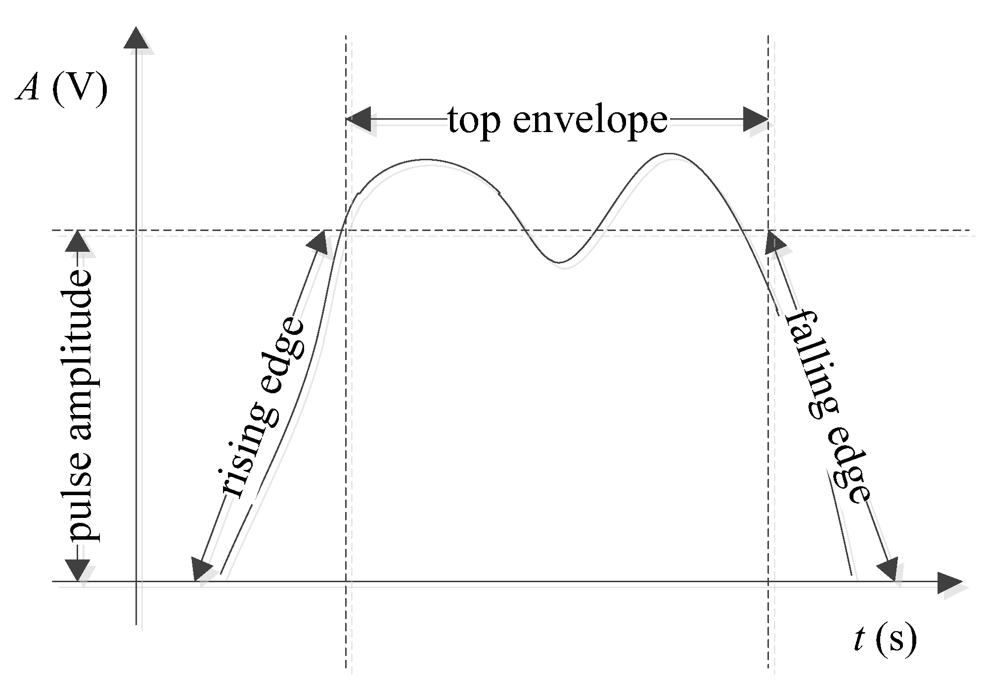
For signal modeling, we mainly consider the influence of phase envelopes, which are a typical emitter signature. The characteristics of a pulse envelope are mainly produced by the following factors: (1) the pulse envelope may be distorted by the inertia of the device during the DAC conversion of a digital signal to an analog signal; (2) the pulse envelope may be distorted by individual differences in the pass band flatness of the low-pass filters and the bandpass filter; this is more obvious for broadband signals, such as linear frequency modulation (LFM) signals; and (3) the pulse envelope can also be distorted by individual differences in frequency response at different frequencies in the pass band of intermediate frequency amplifiers, power amplifiers, etc. The above factors may lead to unsatisfactory envelopes of the pulsed signals from different emitters, which can be regarded as unique signatures of different emitters [26].
A typical envelope of a real pulsed signal is shown in Figure 2. This paper focuses on rising-edge modeling. Both the falling edge and the rising edge are assumed to have a symmetrical shape, and the top envelope is set at a constant level.
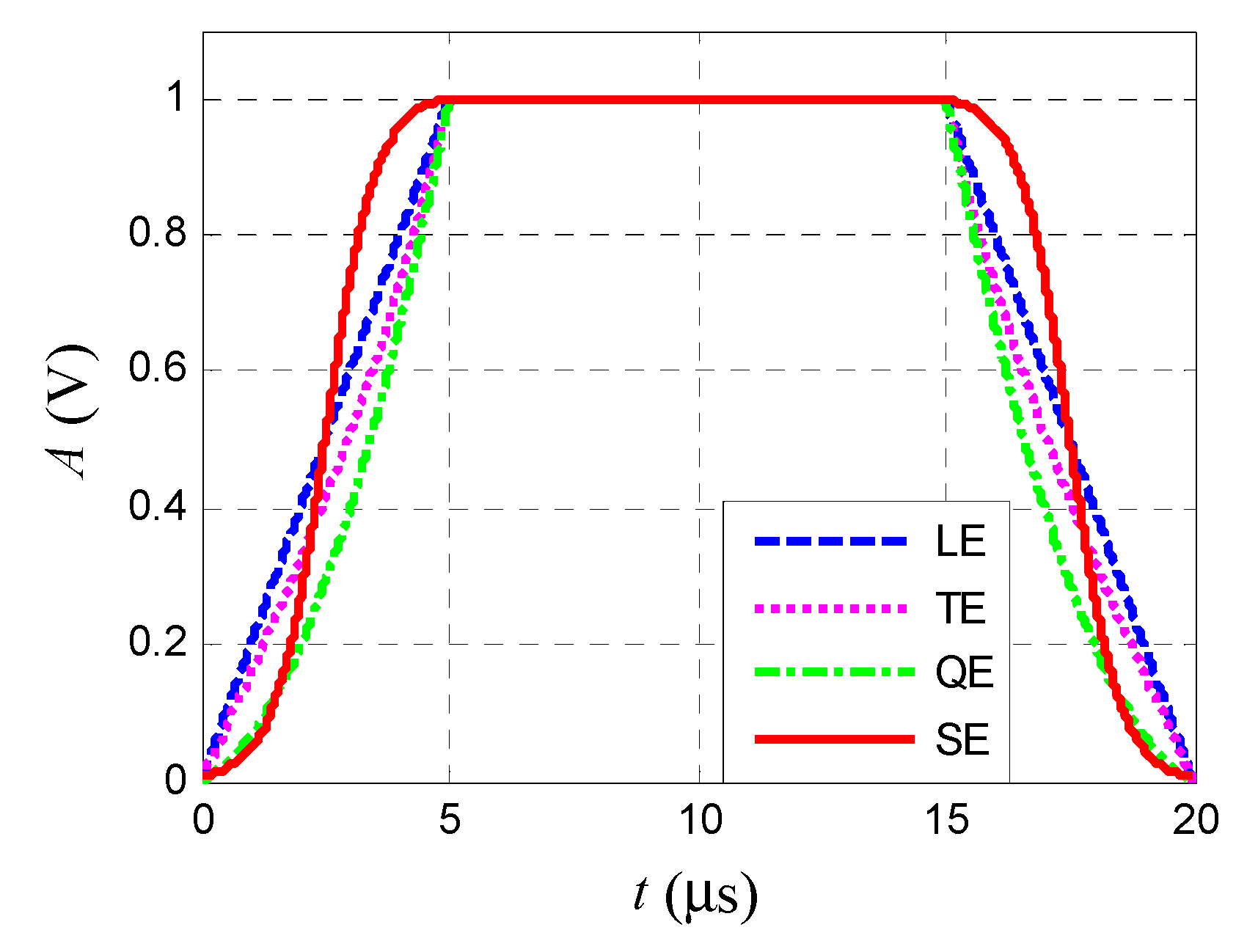
Four types of pulse envelopes were built for this paper, namely, linear envelope (LE), tangent envelope (TE), quadratic envelope (QE), and sigmoid function envelope (SE). The expression for the LE is as follows:
where is the time percentage of the pulse width occupied by the rising edge, which is the same as that occupied by the falling edge if no overshooting occurs.
The expression for the TE is as follows:
where is used to adjust the degree of curvature of the rising edge. Generally, we can set . if no overshooting occurs.
The expression for the QE is as follows:
where a and b are used to adjust the degree of curvature of the rising edge. if no overshooting occurs.
The expression for the SE is as follows:
where is used to adjust the “S” shape of the rising edge. Generally, we can set . if no overshooting occurs.
The differences in the rising edges for different emitters are so small that they can hardly be distinguished considering the transport channel noise, as can be seen from the distance between the different envelopes shown in Figure 3. By inference, SEI will not perform optimally if only some individual features are extracted in the time domain. Therefore, we attempted to extend the time-domain signal in the frequency direction using a signal decomposing algorithm; this can simultaneously increase the dimension of the feature vector in cost and reduce the redundancy of features, which in turn can decrease the feature dimension. As a result, we propose a novel specific emitter identification algorithm which uses individual envelope characteristics. This work was mainly inspired by the distinguished work of Michael A. Temple’s team [6,10,11,12,13,14,15].
3. Proposed Algorithm
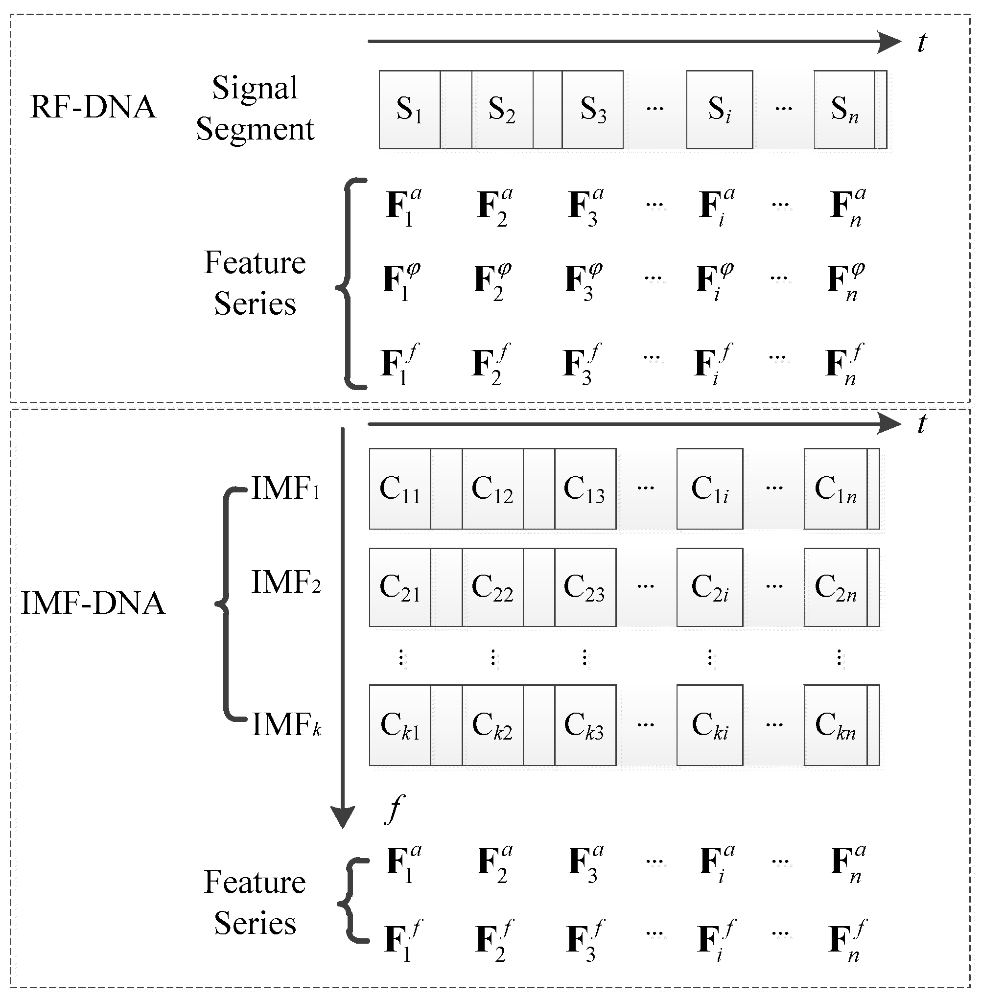
The new algorithm developed in the present study is shown in Figure 4. The algorithm decomposes the original time-domain signal into several IMFs, segments the IMFs into separate time series, and extracts the features that will be used for identification from each IMF. Unlike the RF-DNA algorithm, our algorithm uses features from different IMFs, whose amplitude (a) sequences and frequency (f) sequences are exploited in order to identify specific emitters. Consequently, our algorithm involves far fewer signal segmentations (eight) than the RF-DNA algorithm (80 in [10]). Considering that the feature sources are IMFs, the proposed SEI algorithm is named IMF-DNA.
3.1. Signal Decomposition
A pulsed signal s(t) can be decomposed into
which is a cumulative sum of multiple intrinsic mode functions and a residual trend according to a local feature timescale of the signal, where K is the number of modes. This is the basic idea of EMD, which was proposed by Huang [22]. Recently, it has been shown that the VMD signal decomposing algorithm [23], which is similar to EMD, can also transform a signal into a group of IMFs. Either of these two signal decomposing algorithms is practical for our technical framework. The quantity of IMFs (k) used for fingerprint feature extraction is usually an empirical value depending on the decomposition result, and was set as 3 in the present study. The proposed technical framework also works for the EWT [24].
3.2. IMF Segmentation
In the IMF-DNA algorithm, the IMFs are segmented into several time series, as in the RF-DNA algorithm. The enframe function in the MATLAB software (MathWorks, Natick, MA, USA), which is commonly used for signal windowing and framing in speech signal processing, is a useful tool to segment time sequences, and can be designed as a sliding window to resample the original signal time sequence. Its calling syntax is “y = enframe(x, w, s)”, where x represents the signal to be framed, w is the frame length or window width, and s indicates the step size or sliding window offset. For n segments, we obtain the following:
where the function is the ceiling function, which maps a real number x to the least integer. The returned value y of the enframe function is an matrix, so the fractal dimension needs to be calculated row by row. In this study, the number of segments was 8. The segmentation methodology was presented in our previous paper [21].
3.3. Feature Extraction from IMFs
Following [10], we assume that the individual characteristics for a frequency are duplicates of the features for phase (φ). Therefore, the features are only extracted from the amplitude sequence and the frequency sequence, and the feature structure can be expressed as follows:
where Nc = 4 × nk denotes the number of features extracted from all components (i.e., IMFs) from the amplitude sequence or frequency sequence, respectively; NF = Nc × 2 is the final feature dimension of IMF-DNA; denotes mean value; denotes variance; is skewness; and is kurtosis. In this paper, the final feature dimension of IMF-DNA was 96, compared to a value of 90 for RF-DNA.
3.4. Dimensional Reduction Analysis and the Proposed Joint Feature Selection Algorithm
A previous study [10] used two pre-classification dimensional reduction analysis (DRA) feature selection methods—namely, the Kolmogorov–Smirnov test (KS test) and the F test—and two post-classification DRA feature selection methods—namely, generalized relevance learning vector quantized improved (GRLVQI) relevance and Wilks’s lambda ratio. In the present study, we propose a joint feature selection (JFS) algorithm based on these four feature selection methods (Algorithm 1). This JFS is a voting algorithm and can select the features which contribute most to the classification. The ranking results obtained using the KS test, F test, GRLVQI relevance, and Wilks’s lambda ratio are denoted as K, F, G, and W, respectively.
where Tvoting is a preset threshold value, which is usually more than half the number of all voting members. The degree of feature dimension reduction is denoted as Nd, which refers to the first Nd features of the total number of NF features.
| Algorithm 1: Joint feature selection (JFS) algorithm |
| Initialize the ranking results obtained using each of the four feature selection algorithms (the Kolmogorov–Smirnov test, the F test, GRLVQI relevance, and Wilks’s lambda ratio) as K1×NF, F1×NF, G1×NF, and W1×NF, which stores the feature index number; i = 0; the vote counting result NVC = 01×NF, any element of which is less than or equal to the number of all voting members (4 in this paper); the index number of a group of features selected FS, index number of a group of features to update FS_update Repeat i = i + 1 Count the votes of each feature from the first i numbers of K1×NF, F1×NF, G1×NF and W1×NF, and update NVC Search the elements of NVC and find the feature index members which obtained votes greater than or equal to Tvoting, and denote the result as FS_temp Check the elements of FS_temp, find the new members which do not appear in FS, and denote these new members as FS_update if FS_update is blank continue else FS ← {FS, FS_update} Clear FS_temp FS_update ← 0 until i = NF |
3.5. Recognition Process Using a Support Vector Machine
Support vector machines (SVMs) have been widely used and have generally proven to be powerful and robust classification tools. Therefore, in this study, a classifier based on an SVM was applied for the final emitter identification of SEI. SVMs are machine learning algorithms that are based on statistical learning theory [46] and usually use a kernel function to measure the similarity between two samples and , which can map the nonlinear separable data to a high-dimensional space where the classifier can linearly separate the samples. The decision function for an SVM classifier can be written as follows:
where denotes the i-th sample, i = 1,…, N is the sample index of the training data, and yi = {±1} is the label of each sample. The typical kernels used for SVMs are the Gaussian radial basis function (RBF) kernel, the polynomial kernel, and the sigmoid kernel [47].
SVMs are conventional classifiers for binary classification; however, they can be extended to multiple classification using some algorithms, such as the one-against-all technique. In this study, we exploited a multi-classifier based on the LIBSVM machine learning library [48] to implement the final specific emitter identification, in which a general Gaussian RBF kernel is applied.
4. Numerical Results and Analysis
4.1. Signal Simulation and Feature Extraction
The numerical experiment simulated two emitters, E1 and E2, and three types of primary signals, giving a total of six signal sources, as shown in Table 1. The envelope types could be replaced by QE or SE. The original signal sources can be expressed as follows:
where i = 1,2, Ai(t) is the envelope function designed in Section 2, the initial frequency f0 is 20 MHz, the bandwidth B is 5 MHz, the chirp period T and the pulse width Tw are both 20 μs, and the sampling rate Fs is 1000 MHz. The frequency modulation rate k = B/T, λ = 0.15, and the parameter θ in A2(t) is 0.25π, which can be found in Equation (2). In the equation for s2i(t), φ(t) is the phase modulation function for binary phase shift keying (BPSK) signals, and can be written as follows:
where B(n) denotes a Barker code, Nc is the length of the Barker code, and T is the pulse width, which is 20 μs.
The channel noise type is additive white Gaussian noise, and the number of samples for each emitter and each primary signal type is 1000, resulting in a total of 6000 samples. The signal segmentation number for IMF-DNA is 8, the number of IMFs used for feature extraction is 3, and the feature vector dimension for each IMF segments is 2 with skewness and kurtosis removed. Therefore, the final feature vector dimension is 96. For comparison, the feature vector dimension of RF-DNA is 90 (10 signal segments and 9 features for each segment).
The signal decomposing algorithm used in this paper was VMD, which can effectively separate and suppress the noise component. The key parameter for decomposition, namely K (the total number of modes), was set as 3, and the parameter , which imposes the tightness of the band limits, was set as 1800. The parameter optimization is mainly based on other parameter optimization algorithms, such as particle swarm optimization, which will be presented as a separate work in the future. In this paper, the values of the parameters were obtained by empirical investigation. More details about VMD can be found in [23].
The Tvoting parameter of the proposed feature selection algorithm was set as 4 (i.e., the total number of feature selection methods used for joint selection), and the most recently updated members in one loop were not intentionally ranked again.
4.2. Recognition of Emitters
For the analysis of the classification performance of IMF-DNA and the proposed joint feature selection algorithm, the following three experiments were carried out:
- Experiment 1: Classify the six signal sources into six classes, which means the emitters are identified as six emitters. The experiment was designed to prove that the proposed fingerprint algorithm can also be used for modulation classification;
- Experiment 2: Classify s11, s12, s13 as Emitter E1 and s21, s22, s23 as Emitter E2, that is, identify two different emitters. The experiment was designed to determine the influence of the pulse envelope and primary signal on the proposed fingerprint algorithm;
- Experiment 3: Classify s11 as Emitter E1 and s21 as Emitter E2, which removes the influence of the primary signal and can be used to verify the performance of the SEI using pulse envelope characteristics.
Figure 5 shows the SVM classification performance for six classes for Experiment 1 using the IMF-DNA algorithm. The results proved that the proposed algorithm can effectively distinguish between different modulations with minor differences in individual pulse envelopes. It has previously been shown that the final reduced dimension does not significantly affect the final classification performance [10]. The main reason for this may be that the differences in modulation are large enough to allow correct classification.
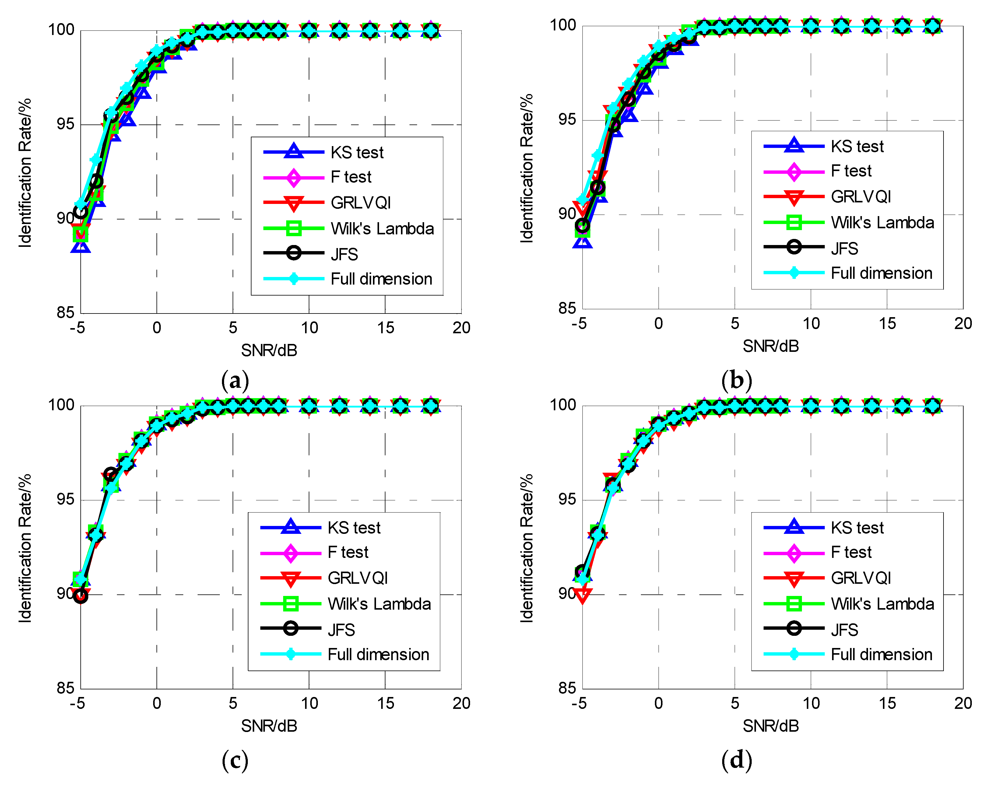
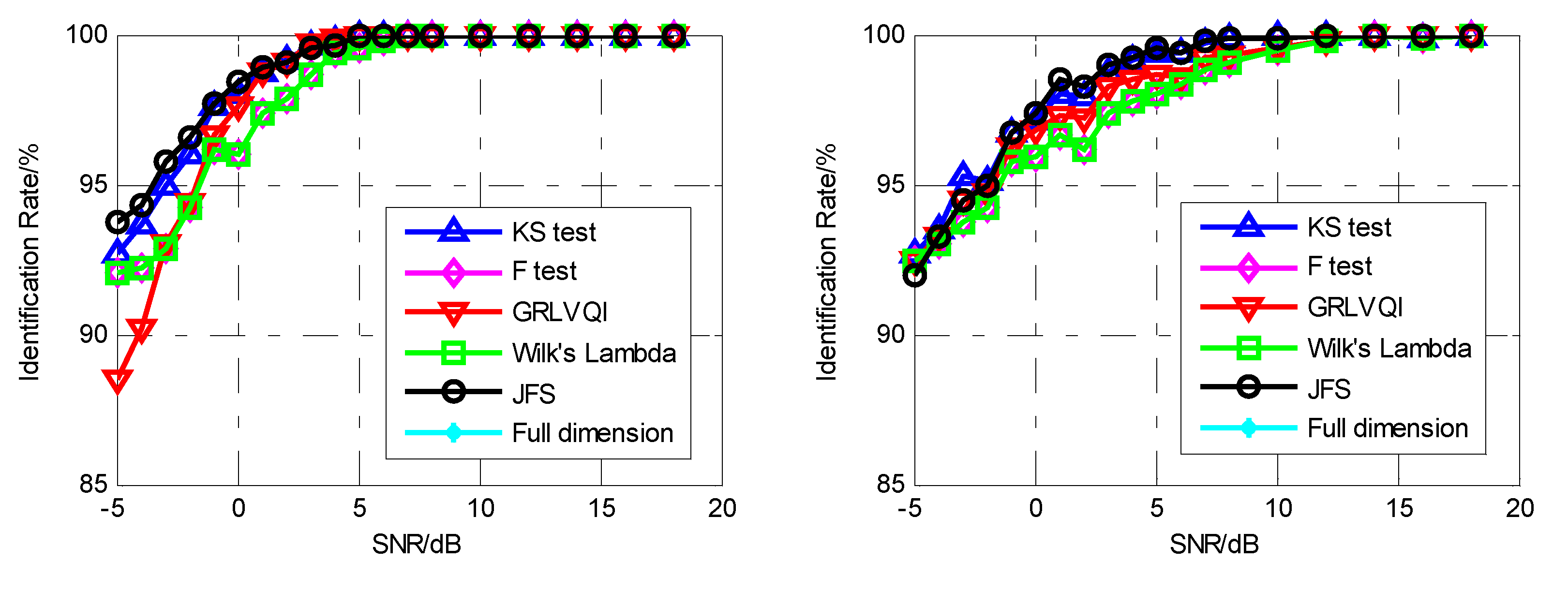
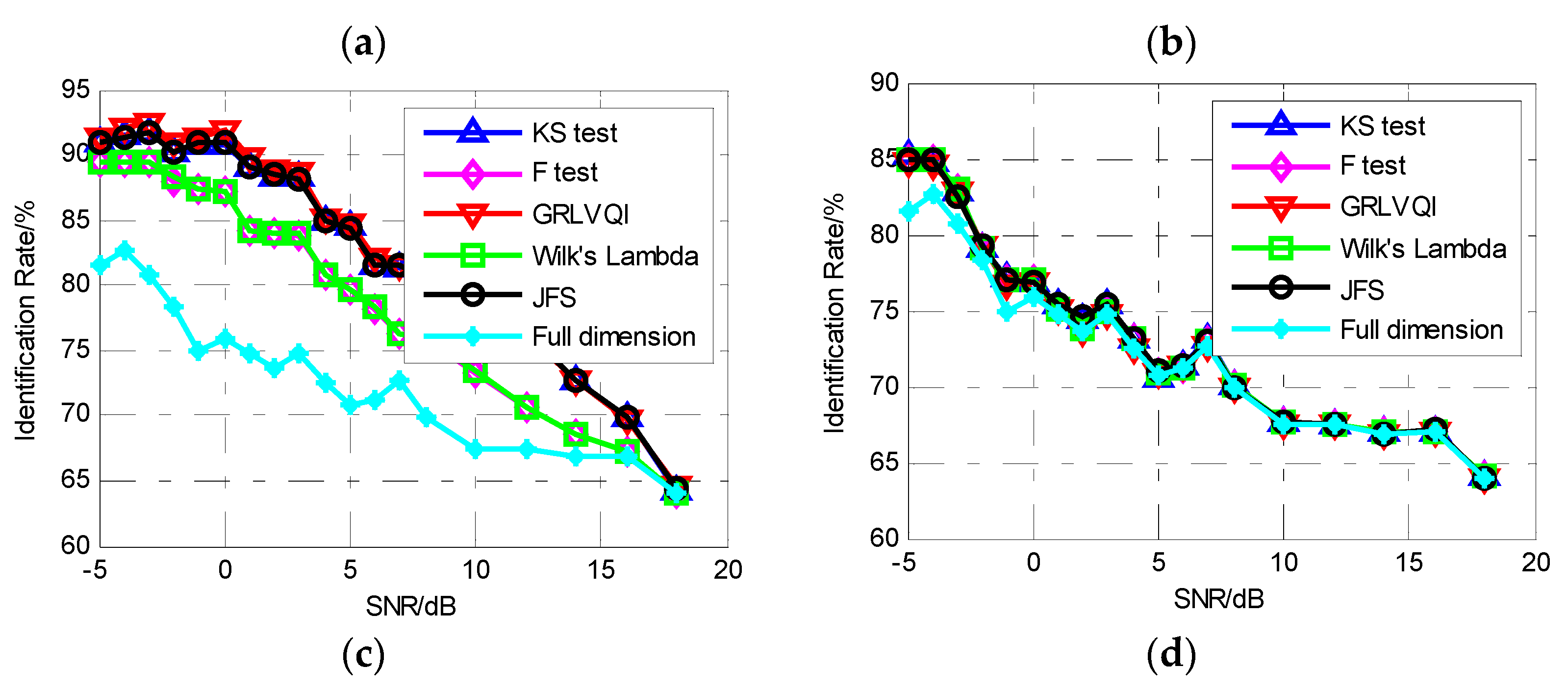
For Experiment 2, simultaneously considering the differences in modulation and the differences between envelopes, it was attempted to use the classification to distinguish the emitters by locating the individual differences between envelopes using the proposed feature selection algorithm. The results are shown in Figure 6. Because features related to the rising edge and falling edge are observed first and the features related to modulation are observed later in the feature selection process, the classification performance is excellent when the reduced dimension is low. As the number of features used for classification increases, during which the ratio of other features related to the modulation also increases, the performance decreases significantly as the difference between the two classes becomes less and less. Especially when SNR increases (Figure 6c,d), the influence of modulation increases rapidly, and consequently the classification performance decreases significantly. Additionally, the full dimension line shown in Figure 6a,b is below 85% and out of the display range of the y-axis, which can be seen in Figure 6c,d.
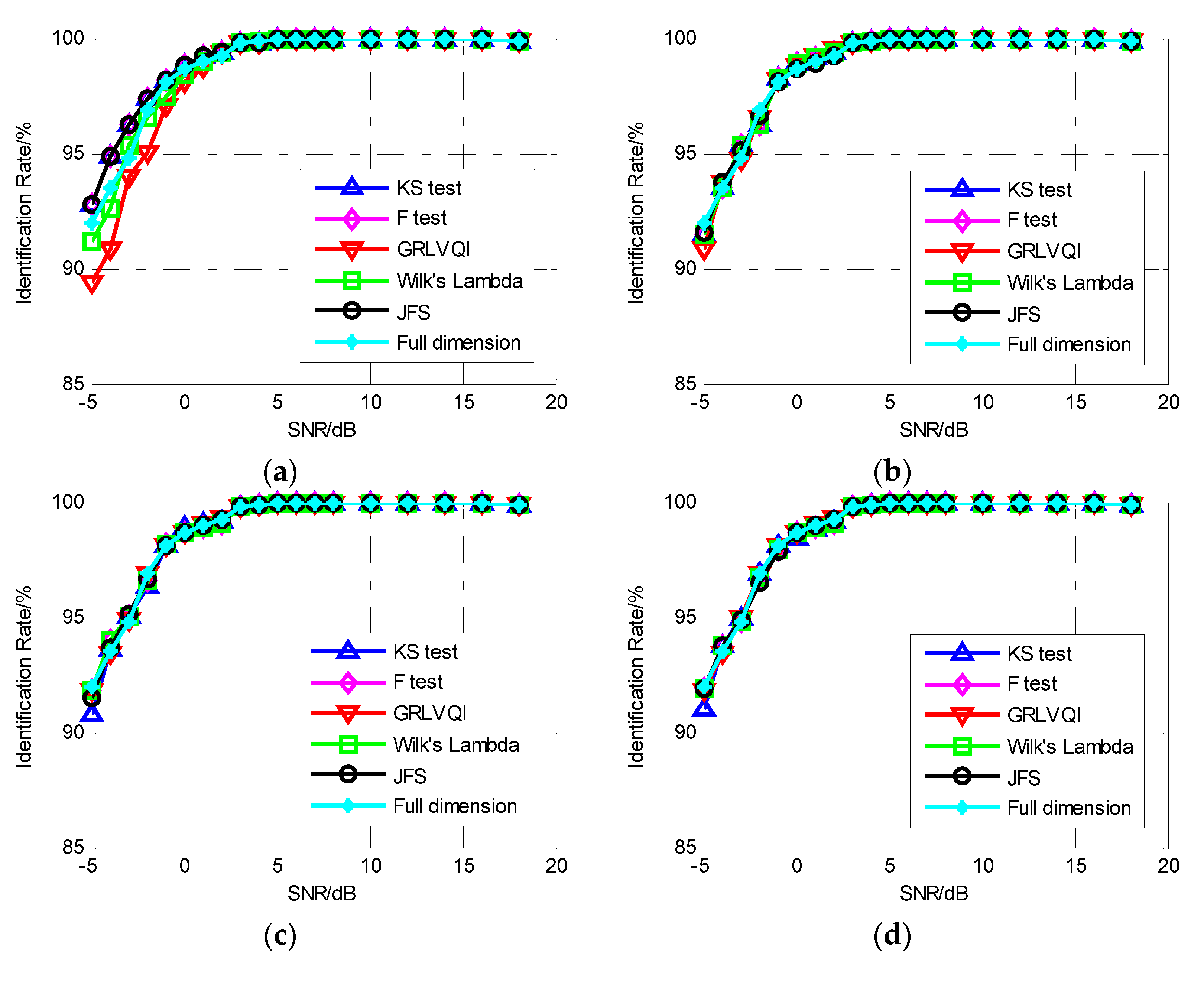
Experiment 3 was designed to remove the influence of the primary signal. Figure 7 shows the results for this experiment in terms of the SVM classification performance for LFMs with different envelopes being classified into two classes using the IMF-DNA algorithm. The result shown in Figure 7a verifies the superior performance of the proposed joint feature selection algorithm compared to the KS test, F test, GRLVQI relevance, and Wilks’s lambda ratio methods. All the primary signals used for classification were LFMs, which means that the differences between primary signals are removed, and the classification performance increases, especially in lower reduced dimensions, such as Nd = 10 (see Figure 5a and Figure 7a). The superior performance of IMF-DNA proves that it can select the ideal features which make the largest contribution to the classification. As the number of features used for the classification increases, the classification performance stays stable, with no differences being observed between primary signals. The above analysis proves the inferences and conclusions in experiment 2 as a supplement.
From the results of experiments 1 to 3, the following conclusions can be made: first, the proposed joint feature selection algorithm performs better than the KS test, F test, GRLVQI relevance, and Wilks’s lambda ratio methods; second, the proposed IMF-DNA algorithm performs excellently for specific emitter identification; and finally, if some primary signal suppression algorithm can remove the influence of the primary signal on the specific emitter features, the SEI performance will increase more robustly, which can prevent the performance reduction observed in Experiment 2. Future work will involve exploiting a primary signal suppression algorithm for SEI.
4.3. Comparison between IMF-DNA and RF-DNA
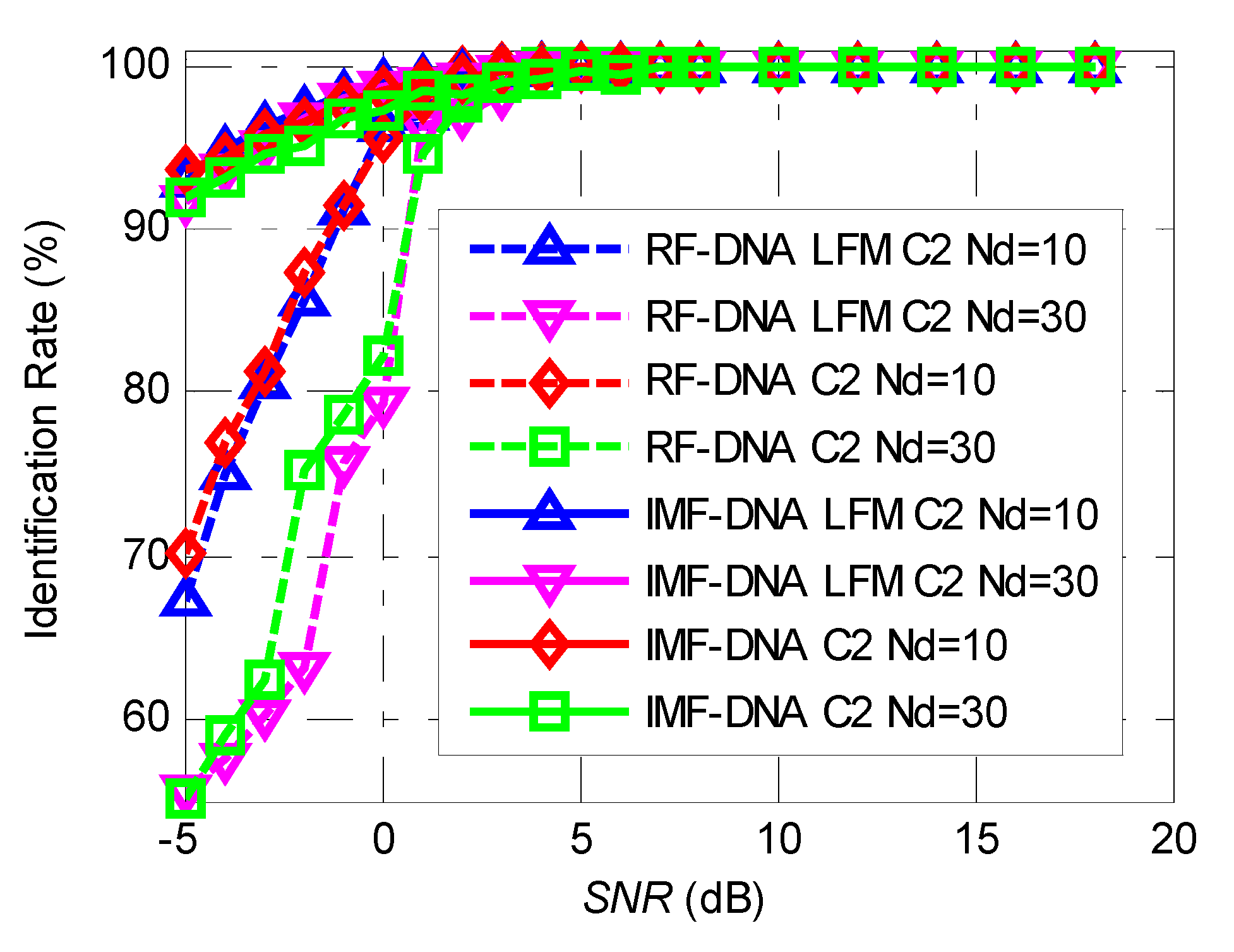
For a final performance comparison, the RF-DNA feature vector was designed as a 90-dimensional vector, consisting of 10 signal segments each containing 9 feature vector members. This high dimensional vector was reduced into 10 or 30 dimensions using the proposed joint feature selection algorithm. The final performance comparison between IMF-DNA and RF-DNA is shown in Figure 8.
As can be seen from Figure 8, the performance of the IMF-DNA algorithm is much better than that of RF-DNA, especially for lower SNR. The main reason why IMF-DNA performs better is that the VMD algorithm can decompose the original signal into several IMFs and the original minor differences in envelope will be distributed in different IMFs, which makes it possible for some differences to become more outstanding when other components are removed. At the same time, an efficient feature selection algorithm was applied to find the features which contribute most to the classification, which maximizes the distance between classes.
When using the proposed algorithm, we found that the sampling rate also affects the classification performance. Specific emitter identification performs better with a higher sampling rate, which requires more calculation.
5. Verification Using Real Data
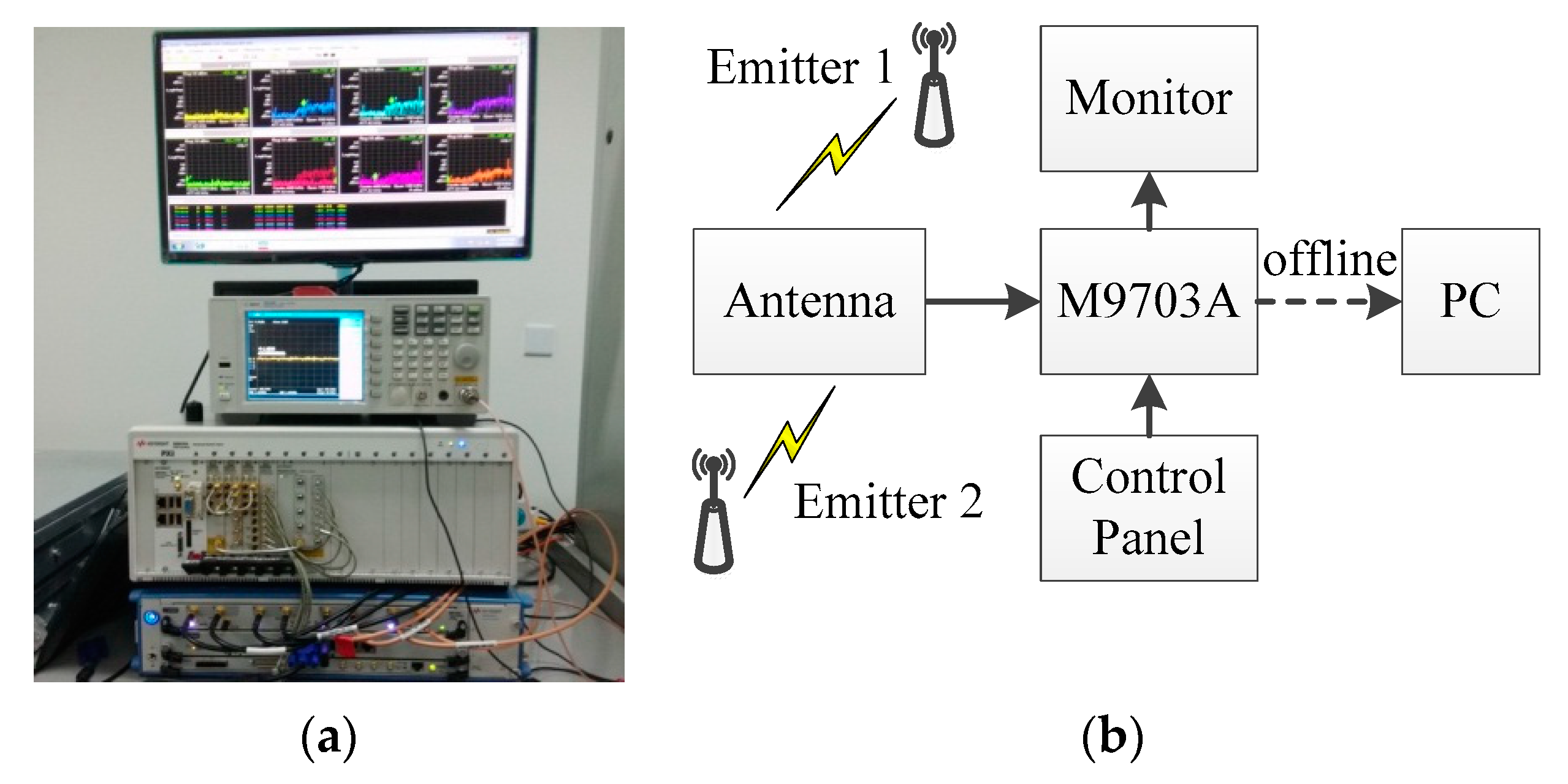
To verify the performance and practicality of the proposed algorithm, the emitted signals from two signal sources of the same type were sampled. To suppress the influence of the sampling equipment, this study used an M9703A high-speed digitizer/wideband digital receiver (Keysight Technologies, Inc., Santa Rosa, CA, USA), which had been regulated within the last year, to sample the signal sources. The real signal sampling experiment is described in Figure 9. The sampling work was presented in our previous paper [21].
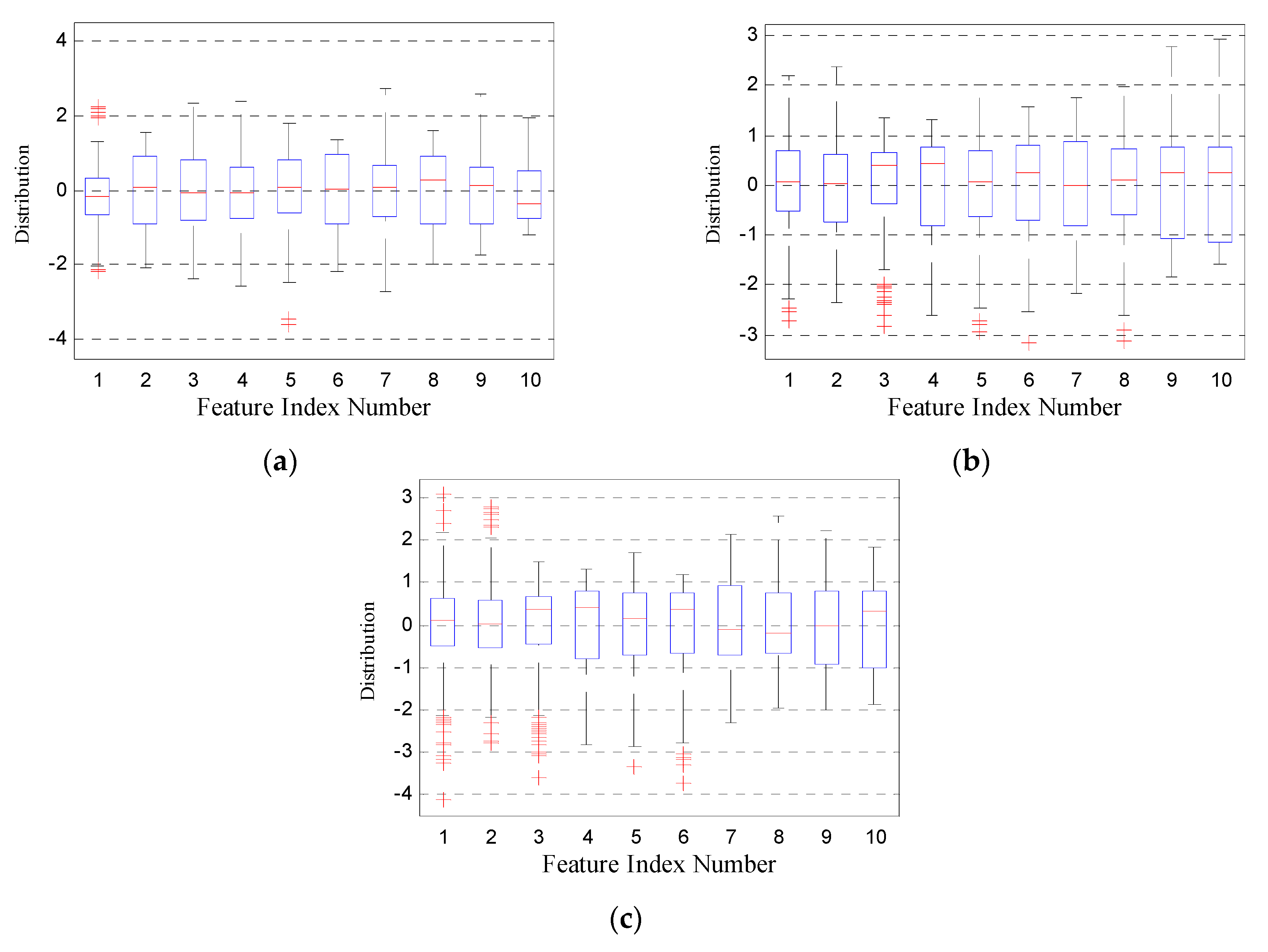
The carrier frequency of the two emitters was 425 MHz, the modulation bandwidth was 5 MHz, and the pulse width was 130 μs. The sampling rate was 2 GHz and the digital down-conversion process moved the spectrum to the intermediate frequency of 25 MHz. A total of 1000 samples for each emitter with similar values of estimated SNR were selected. Other real radar emitter sampling data, with a sampling rate of 200 MHz, were incorporated into the identification process. Therefore, the down-sampling rate for the first two signal sources was also set to 200 MHz. A total of 1000 pulses from the real radar emitter were selected for identification at the same time. Figure 10 presents the feature distribution of the three different real emitters after normalization; the data have a mean value of zero and a variance of 1.
As shown in Figure 10, Emitters 1 and 2 are signal sources with more stable parameters, which makes the feature distribution more stable and the spectrum purer. Emitter 3 is a real radar emitter with more outliers distributed at both ends, especially in features 1 to 6, which indicates strong dispersion characteristics.
For the final identification, 30% of the samples were used for training and the rest of the samples were used for testing. The SNR was estimated to be approximately 10.0 dB, and the correct identification rate was 85.3% using the proposed SEI algorithm, which consists of the IMF-DNA fingerprint algorithm and a joint feature selection algorithm. For comparison, the correct identification rate using RF-DNA under almost the same conditions was 83.3%. The final correct identification rate is different from the simulation result shown in Figure 8, which is mainly due to the sampling rate.
6. Conclusions
In this paper, individual differences in pulse envelopes were analyzed and four types of pulse envelopes were modeled. After the signal modeling, a specific emitter identification algorithm using IMF-DNA and a joint feature selection algorithm was proposed. Compared to four other feature selection methods, the proposed feature selection algorithm performed better, finding the most useful features for classification, which significantly helped with the reduction of feature dimension. Three experiments were used to verify the practical performance of IMF-DNA for modulation recognition and specific emitter identification. Compared with RF-DNA, IMF-DNA achieved a higher correct emitter identification rate under similar conditions in simulation experiments. IMF-DNA has significant advantages over RF-DNA, especially for lower SNRs (e.g., below 0 dB). On the other hand, for SNRs above 0 dB, the performances of the two algorithms rapidly converged, and they eventually became equal. However, for real data verification, the correct identification rate of IMF-DNA was only marginally higher than that of RF-DNA, which was mainly due to the sampling rate. Real data verification proved that the practical performance of IMF-DNA for specific emitter identification is excellent; the algorithm achieved a correct identification rate of 85.3% at a sampling rate of 200 MHz and an estimated SNR of approximately 10 dB.
Author Contributions
All authors contributed to this work. Conceptualization, L.W. and Y.Z.; methodology, L.W.; software, L.W. and M.F.; validation, Y.Z.; formal analysis, L.W. and Y.Z.; investigation, M.F., F.Y.O.A., and H.U.; data curation, L.W.; writing—original draft preparation, L.W.; writing—review and editing, L.W., Y.Z., F.Y.O.A., and H.U.; visualization, L.W.; supervision, Y.Z.; project administration, Y.Z.; funding acquisition, Y.Z.
Funding
This research was funded by the National Natural Science Foundation of China, grant number 61671185.
Acknowledgments
The authors would like to thank the anonymous reviewers for their patience and helpful comments to improve our paper. They also wish to thank Robin Wylie for improving the language of our paper.
Conflicts of Interest
The authors declare no conflict of interest. The funders had no role in the design of the study; in the collection, analyses, or interpretation of data; in the writing of the manuscript; or in the decision to publish the results.
References
- Langley, L.E. Specific emitter identification (SEI) and classical parameter fusion technology. In Proceedings of the WESCON/’93, San Francisco, CA, USA, 28–30 September 1993; pp. 377–381. [Google Scholar]
- Talbot, K.I.; Duley, P.R.; Hyatt, M.H. Specific emitter identification and verification. Technol. Rev. J. 2003, 113–133. [Google Scholar]
- Stove, A.G.; Hume, A.L.; Baker, C.J. Low probability of intercept radar strategies. IEE Proc. Radar Sonar Navig. 2004, 151, 249. [Google Scholar] [CrossRef]
- Krishnamurthy, V. Emission management for low probability intercept sensors in network centric warfare. IEEE Trans. Aerosp. Electron. Syst. 2005, 41, 133–152. [Google Scholar] [CrossRef]
- Lee, K.-W.; Lee, W.-K. The Low Probability of Intercept RADAR Waveform Based on Random Phase and Code Rate Transition for Doppler Tolerance Improvement. J. Korean Inst. Electromagn. Eng. Sci. 2015, 26, 999–1011. [Google Scholar] [CrossRef]
- Rondeau, C.M.; Betances, J.A.; Temple, M.A. Securing ZigBee Commercial Communications Using Constellation Based Distinct Native Attribute Fingerprinting. Secur. Commun. Netw. 2018, 2018. [Google Scholar] [CrossRef]
- Lopez, J.; Liefer, N.C.; Busho, C.R.; Temple, M.A. Enhancing Critical Infrastructure and Key Resources (CIKR) Level-0 Physical Process Security Using Field Device Distinct Native Attribute Features. IEEE Trans. Inf. Forensic Secur. 2018, 13, 1215–1229. [Google Scholar] [CrossRef]
- Zhang, J.W.; Cabric, D.; Wang, F.G.; Zhong, Z.D. Cooperative Modulation Classification for Multipath Fading Channels via Expectation-Maximization. IEEE Trans. Wirel. Commun. 2017, 16, 6698–6711. [Google Scholar] [CrossRef]
- Zhang, J.; Wang, F.; Dobre, O.A.; Zhong, Z. Specific Emitter Identification via Hilbert-Huang Transform in Single-Hop and Relaying Scenarios. IEEE Trans. Inf. Forensic Secur. 2016, 11, 1192–1205. [Google Scholar] [CrossRef]
- Bihl, T.J.; Bauer, K.W.; Temple, M.A. Feature Selection for RF Fingerprinting With Multiple Discriminant Analysis and Using ZigBee Device Emissions. IEEE Trans. Inf. Forensic Secur. 2016, 11, 1862–1874. [Google Scholar] [CrossRef]
- Patel, H.J.; Temple, M.A.; Baldwin, R.O. Improving ZigBee Device Network Authentication Using Ensemble Decision Tree Classifiers With Radio Frequency Distinct Native Attribute Fingerprinting. IEEE Trans. Rel. 2015, 64, 221–233. [Google Scholar] [CrossRef]
- Lukacs, M.; Collins, P.; Temple, M. Classification performance using ’RF-DNA’ fingerprinting of ultra-wideband noise waveforms. Electron. Lett. 2015, 51, 787–788. [Google Scholar] [CrossRef]
- Dubendorfer, C.; Ramsey, B.; Temple, M. ZigBee Device Verification for Securing Industrial Control and Building Automation Systems. In Critical Infrastructure Protection VII: 7th IFIP WG 11.10 International Conference, ICCIP 2013, Washington, DC, USA, March 18–20, 2013, Revised Selected Papers; Butts, J., Shenoi, S., Eds.; Springer Berlin Heidelberg: Berlin/Heidelberg, Germany, 2013; pp. 47–62. [Google Scholar] [CrossRef] [Green Version]
- Dubendorfer, C.K.; Ramsey, B.W.; Temple, M.A. An RF-DNA verification process for ZigBee networks. In Proceedings of the MILCOM 2012–2012 IEEE Military Communications Conference, Orlando, FL, USA, 29 October–1 November 2012; pp. 1–6. [Google Scholar]
- Cobb, W.E.; Garcia, E.W.; Temple, M.A.; Baldwin, R.O.; Kim, Y.C. Physical Layer Identification of Embedded Devices Using RF-DNA Fingerprinting. In Proceedings of the 2010 - MILCOM 2010 MILITARY COMMUNICATIONS CONFERENCE, San Jose, CA, USA, 31 October–3 November 2010. [Google Scholar] [CrossRef]
- Suski II, W.C.; Temple, M.A.; Mendenhall, M.J.; Mills, R.F. Radio frequency fingerprinting commercial communication devices to enhance electronic security. Int. J. Electron. Secur. Digit. Forensic 2008, 1, 301–322. [Google Scholar] [CrossRef]
- Liu, M.-W.; Doherty, J.F. Nonlinearity Estimation for Specific Emitter Identification in Multipath Environment. In Proceedings of the 2009 IEEE Sarnoff Symposium, Princeton, NJ, USA, 30 March–1 April 2009. [Google Scholar] [CrossRef]
- Dudczyk, J.; Kawalec, A. Identification of emitter sources in the aspect of their fractal features. Bull. Pol. Acad. Sci. Tech. Sci. 2013, 61, 623–628. [Google Scholar] [CrossRef] [Green Version]
- Tang, Z.; Li, S. Steady Signal-Based Fractal Method of Specific Communications Emitter Sources Identification. In Wireless Communications, Networking and Applications, Wcna 2014; Zeng, Q.A., Ed.; Springer: New Delhi, India, 2016; Vol. 348, pp. 809–819. [Google Scholar]
- Huang, G.; Yuan, Y.; Wang, X.; Huang, Z. Specific Emitter Identification Based on Nonlinear Dynamical Characteristics. Canadian J. Electric. Comput. Eng. Rev. Canad. Genie Electriq. Inform. 2016, 39, 34–41. [Google Scholar] [CrossRef]
- Wu, L.; Zhao, Y.; Wang, Z.; Abdalla, F.Y.O.; Ren, G. Specific emitter identification using fractal features based on box-counting dimension and variance dimension. In Proceedings of the 2017 IEEE International Symposium on Signal Processing and Information Technology (ISSPIT), 1 Bilbao, Spain, 8–20 December 2017; pp. 226–231. [Google Scholar]
- Huang, N.E.; Shen, Z.; Long, S.R.; Wu, M.L.C.; Shih, H.H.; Zheng, Q.N.; Yen, N.C.; Tung, C.C.; Liu, H.H. The empirical mode decomposition and the Hilbert spectrum for nonlinear and non-stationary time series analysis. Proc. R. Soc. London, Ser. A 1998, 454, 903–995. [Google Scholar] [CrossRef]
- Dragomiretskiy, K.; Zosso, D. Variational Mode Decomposition. Ieee Trans. Sign. Proc. 2014, 62, 531–544. [Google Scholar] [CrossRef]
- Gilles, J. Empirical Wavelet Transform. IEEE Trans. Sign. Proc. 2013, 61, 3999–4010. [Google Scholar] [CrossRef]
- Satija, U.; Trivedi, N.; Biswal, G.; Ramkumar, B. Specific Emitter Identification Based on Variational Mode Decomposition and Spectral Features in Single Hop and Relaying Scenarios. IEEE Trans. Inf. Forensic Secur. 2019, 14, 581–591. [Google Scholar] [CrossRef]
- Yuan, Y.; Huang, Z.; Wu, H.; Wang, X. Specific emitter identification based on Hilbert-Huang transform-based time-frequency-energy distribution features. IET Commun. 2014, 8, 2404–2412. [Google Scholar] [CrossRef]
- Gok, G.; Alp, Y.K.; Altiparmak, F. Radar Fingerprint Extraction via Variational Mode Decomposition. In Proceedings of the 2017 25th Signal Processing and Communications Applications Conference (Siu), Antalya, Turkey, 15–18 May 2017. [Google Scholar]
- Li, Y.; Chen, X.; Yu, J.; Yang, X. A Fusion Frequency Feature Extraction Method for Underwater Acoustic Signal Based on Variational Mode Decomposition, Duffing Chaotic Oscillator and a Kind of Permutation Entropy. Electronics 2019, 8. [Google Scholar] [CrossRef]
- Gao, J.; Shen, L.; Gao, L.; Lu, Y. A Rapid Accurate Recognition System for Radar Emitter Signals. Electronics 2019, 8. [Google Scholar] [CrossRef]
- Huang, Y.; Bao, H.; Qi, X. Seismic Random Noise Attenuation Method Based on Variational Mode Decomposition and Correlation Coefficients. Electronics 2018, 7. [Google Scholar] [CrossRef]
- Zhao, Y.; Wu, L.; Zhang, J.; Li, Y. Specific emitter identification using geometric features of frequency drift curve. Bull. Pol. Acad. Sci., Chem. 2018, 66, 99–108. [Google Scholar] [CrossRef]
- Ye, H.; Liu, Z.; Jiang, W. Comparison of unintentional frequency and phase modulation features for specific emitter identification. Electronics Lett. 2012, 48, 875–876. [Google Scholar] [CrossRef]
- Wisell, D.H.; Rudlund, B.; Ronnow, D. Characterization of Memory Effects in Power Amplifiers Using Digital Two-Tone Measurements. IEEE Trans. Instrum. Meas. 2007, 56, 2757–2766. [Google Scholar] [CrossRef]
- Harmer, P.K.; Reising, D.R.; Temple, M.A. Classifier selection for physical layer security augmentation in Cognitive Radio networks. In Proceedings of the 2013 IEEE International Conference on Communications (ICC), Budapest, Hungary, 9–13 June 2013; pp. 2846–2851. [Google Scholar]
- Dudczyk, J.; Kawalec, A. Fast-decision identification algorithm of emission source pattern in database. Bull. Pol. Acad. Sci. Techn. Sci. 2015, 63, 385–389. [Google Scholar] [CrossRef] [Green Version]
- Dudczyk, J.; Kawalec, A. Specific emitter identification based on graphical representation of the distribution of radar signal parameters. Bull. Pol. Acad. Sci. Techn. Sci. 2015, 63, 391–396. [Google Scholar] [CrossRef]
- Kawalec, A.; Owczarek, R.; Dudczyk, J. Data modeling and simulation applied to radar signal recognition. Mol. Quantum Acoust. 2005, 26, 165–173. [Google Scholar]
- Kawalec, A.; Owczarek, R. Specific emitter identification using intrapulse data. In Proceedings of the First European Radar Conference, 2004. EURAD, Amsterdam, The Netherlands, 11–15 October 2004; pp. 249–252. [Google Scholar]
- Jiang, H.; Guan, W.; Ai, L. Specific Radar Emitter Identification Based on a Digital Channelized Receiver. In Proceedings of the 2012 5th International Congress on Image and Signal Processing, Chongqing, China, 16–18 October 2012. [Google Scholar]
- Samborski, R.; Ziolko, M. Speaker Localization in Conferencing Systems Employing Phase Features and Wavelet Transform. In Proceedings of the IEEE International Symposium on Signal Processing and Information Technology, Athens, Greece, 12–15 December 2013. [Google Scholar]
- Chen, T.W.; Jin, W.D.; Li, J. Feature Extraction Using Surrounding-Line Integral Bispectrum for Radar Emitter signal. In Proceedings of the 2008 IEEE International Joint Conference on Neural Networks (IEEE World Congress on Computational Intelligence), Hong Kong, China, 1–8 June 2008. [Google Scholar]
- Shi, Y.; Ji, H. Kernel canonical correlation analysis for specific radar emitter identification. Electronics Lett. 2014, 50, 1318–1319. [Google Scholar] [CrossRef]
- Aubry, A.; Bazzoni, A.; Carotenuto, V.; De Maio, A.; Failla, P. Cumulants-based Radar Specific Emitter Identification. In Proceedings of the 2011 IEEE International Workshop on Information Forensics and Security, Iguacu Falls, Brazil, 29 November–2 December 2011. [Google Scholar]
- Matuszewski, J. Specific emitter identification. In Proceedings of the 2008 International Radar Symposium, Wroclaw, Poland, 21–23 May 2008. [Google Scholar]
- Kawalec, A.; Owczarek, R. Radar emitter recognition using intrapulse data. In Proceedings of the 15th International Conference on Microwaves, Radar and Wireless Communications (IEEE Cat. No.04EX824), Warsaw, Poland, 17–19 May 2004. [Google Scholar]
- Burges, C.J.C. A tutorial on Support Vector Machines for pattern recognition. Data Min. Knowl. Disc. 1998, 2, 121–167. [Google Scholar] [CrossRef]
- Gonen, M.; Alpaydin, E. Multiple Kernel Learning Algorithms. J. Mach. Learn. Res. 2011, 12, 2211–2268. [Google Scholar]
- Chang, C.-C.; Lin, C.-J. LIBSVM: A library for support vector machines. ACM Trans. Intell. Syst. Technol. 2011, 2, 1–27. [Google Scholar] [CrossRef]
Figure 1.
The schematic timing diagram of a receiver and an emitter. OTU, observing time unit; A/D, analog/digital.
Figure 1.
The schematic timing diagram of a receiver and an emitter. OTU, observing time unit; A/D, analog/digital.

Figure 2.
A typical envelope of a pulsed signal.

Figure 3.
The four types of pulse envelopes used in this study.

Figure 4.
The comparison of the process flows of the proposed specific emitter identification (SEI) using the intrinsic mode function distinct native attribute (IMF-DNA) algorithm and the radio frequency DNA (RF-DNA) algorithm.
Figure 4.
The comparison of the process flows of the proposed specific emitter identification (SEI) using the intrinsic mode function distinct native attribute (IMF-DNA) algorithm and the radio frequency DNA (RF-DNA) algorithm.

Figure 5.
The performance of the support vector machine (SVM) classification for six classes using IMF-DNA. (a) Nd = 10. (b) Nd = 30. (c) Nd = 50. (d) Nd = 80.
Figure 5.
The performance of the support vector machine (SVM) classification for six classes using IMF-DNA. (a) Nd = 10. (b) Nd = 30. (c) Nd = 50. (d) Nd = 80.

Figure 6.
The SVM classification performance for two classes using the IMF-DNA algorithm. (a) Nd = 10. (b) Nd = 30. (c) Nd = 50. (d) Nd = 80.
Figure 6.
The SVM classification performance for two classes using the IMF-DNA algorithm. (a) Nd = 10. (b) Nd = 30. (c) Nd = 50. (d) Nd = 80.


Figure 7.
The performance of the SVM classification for linear frequency modulations (LFMs) with different envelopes being classified into two classes using IMF-DNA. (a) Nd = 10. (b) Nd = 30. (c) Nd = 50. (d) Nd = 80.
Figure 7.
The performance of the SVM classification for linear frequency modulations (LFMs) with different envelopes being classified into two classes using IMF-DNA. (a) Nd = 10. (b) Nd = 30. (c) Nd = 50. (d) Nd = 80.

Figure 8.
A comparison of the identification performance of the RF-DNA and IMF-DNA algorithms for LFMs with different envelopes being classified into two classes and all the signal sources being classified into two classes.
Figure 8.
A comparison of the identification performance of the RF-DNA and IMF-DNA algorithms for LFMs with different envelopes being classified into two classes and all the signal sources being classified into two classes.

Figure 9.
Real signal sampling experiment. (a) Sampling the signals from two emitters. (b) Process of signal sampling and signal processing.
Figure 9.
Real signal sampling experiment. (a) Sampling the signals from two emitters. (b) Process of signal sampling and signal processing.

Figure 10.
The feature distribution of three different real emitters after normalization. (a) Emitter 1. (b) Emitter 2. (c) Emitter 3 (real radar emitter).
Figure 10.
The feature distribution of three different real emitters after normalization. (a) Emitter 1. (b) Emitter 2. (c) Emitter 3 (real radar emitter).


Table 1.
The signal parameters used for different pulse envelopes. LE, linear envelope; TE, tangent envelope; LFM, linear frequency modulation; BPSK, binary phase shift keying.
Table 1.
The signal parameters used for different pulse envelopes. LE, linear envelope; TE, tangent envelope; LFM, linear frequency modulation; BPSK, binary phase shift keying.
| Emitter | Envelope Type | Primary Signal Type | ||
|---|---|---|---|---|
| LFM | BPSK | Single Tone | ||
| E1 | LE | s11 | s21 | s31 |
| E2 | TE | s12 | s22 | s32 |
© 2019 by the authors. Licensee MDPI, Basel, Switzerland. This article is an open access article distributed under the terms and conditions of the Creative Commons Attribution (CC BY) license (http://creativecommons.org/licenses/by/4.0/).
Share and Cite
MDPI and ACS Style
Wu, L.; Zhao, Y.; Feng, M.; Abdalla, F.Y.O.; Ullah, H. Specific Emitter Identification Using IMF-DNA with a Joint Feature Selection Algorithm. Electronics 2019, 8, 934. https://doi.org/10.3390/electronics8090934
AMA Style
Wu L, Zhao Y, Feng M, Abdalla FYO, Ullah H. Specific Emitter Identification Using IMF-DNA with a Joint Feature Selection Algorithm. Electronics. 2019; 8(9):934. https://doi.org/10.3390/electronics8090934
Chicago/Turabian StyleWu, Longwen, Yaqin Zhao, Mengfei Feng, Fakheraldin Y. O. Abdalla, and Hikmat Ullah. 2019. "Specific Emitter Identification Using IMF-DNA with a Joint Feature Selection Algorithm" Electronics 8, no. 9: 934. https://doi.org/10.3390/electronics8090934
Note that from the first issue of 2016, this journal uses article numbers instead of page numbers. See further details here.