Predictor-Based Motion Tracking Control for Cloud Robotic Systems with Delayed Measurements


Abstract
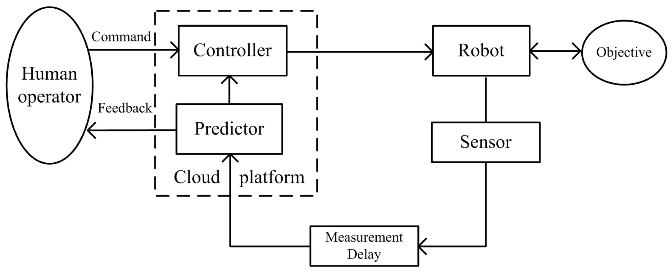
:1. Introduction
2. Problem Statement
- Property 1:
- The inertia matrix is definitely positive. There exist the positive constants and such that , where I is an identity matrix.
- Property 2:
- The matrix is skew symmetric.
- Property 3:
- There exists a positive scalar c such that .
- Assumption 1:
- The desired trajectory is designed such that the time derivative of exist and are bounded by known positive constants.
- Assumption 2:
- is an function.
- Assumption 3:
- Assumption 4:
- The unknown part with its time derivative are bounded functions and satisfy
3. Predictor Design
3.1. Predictor Formulation
3.2. Prediction Error Analysis
4. Controller Development
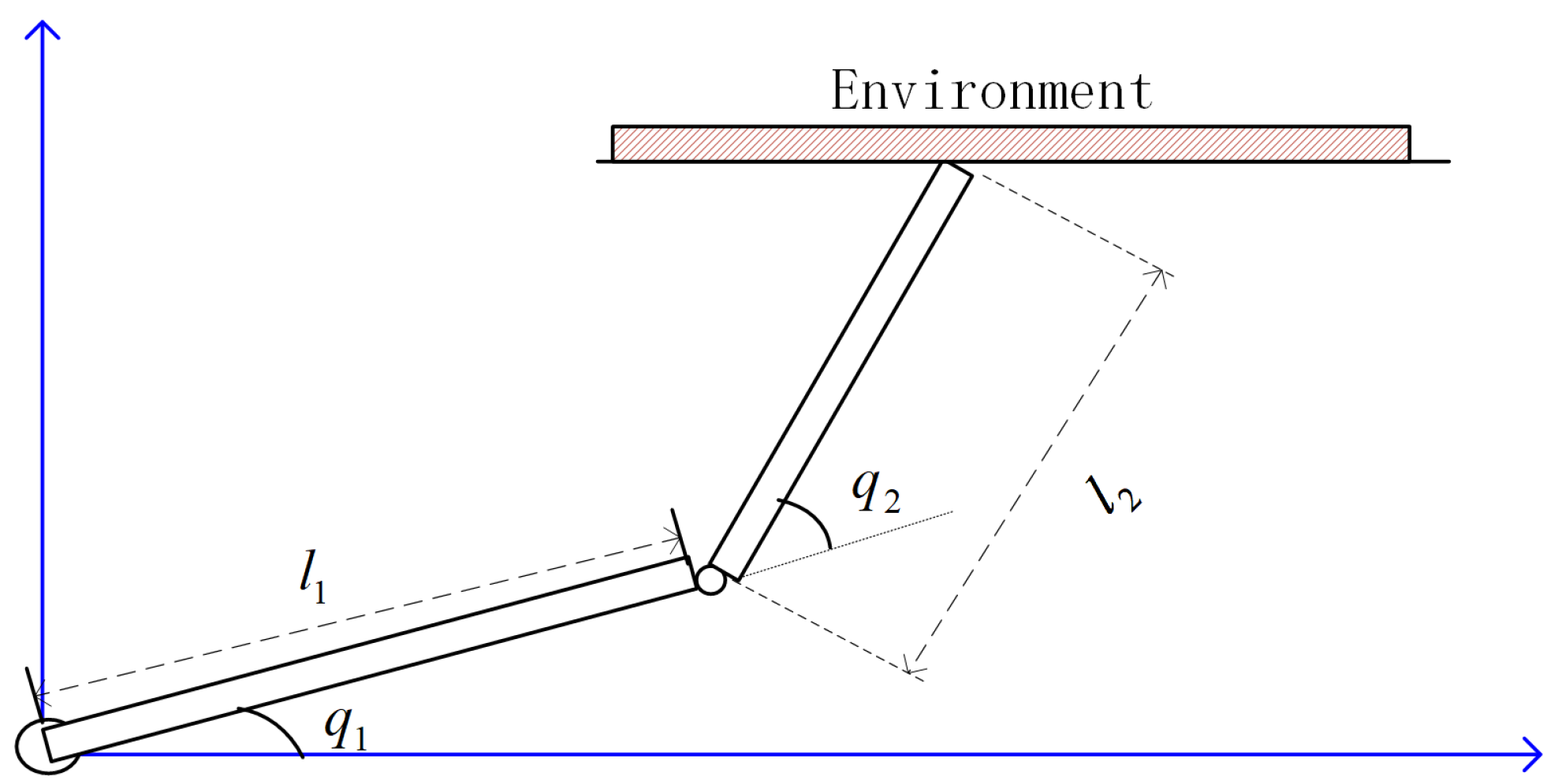
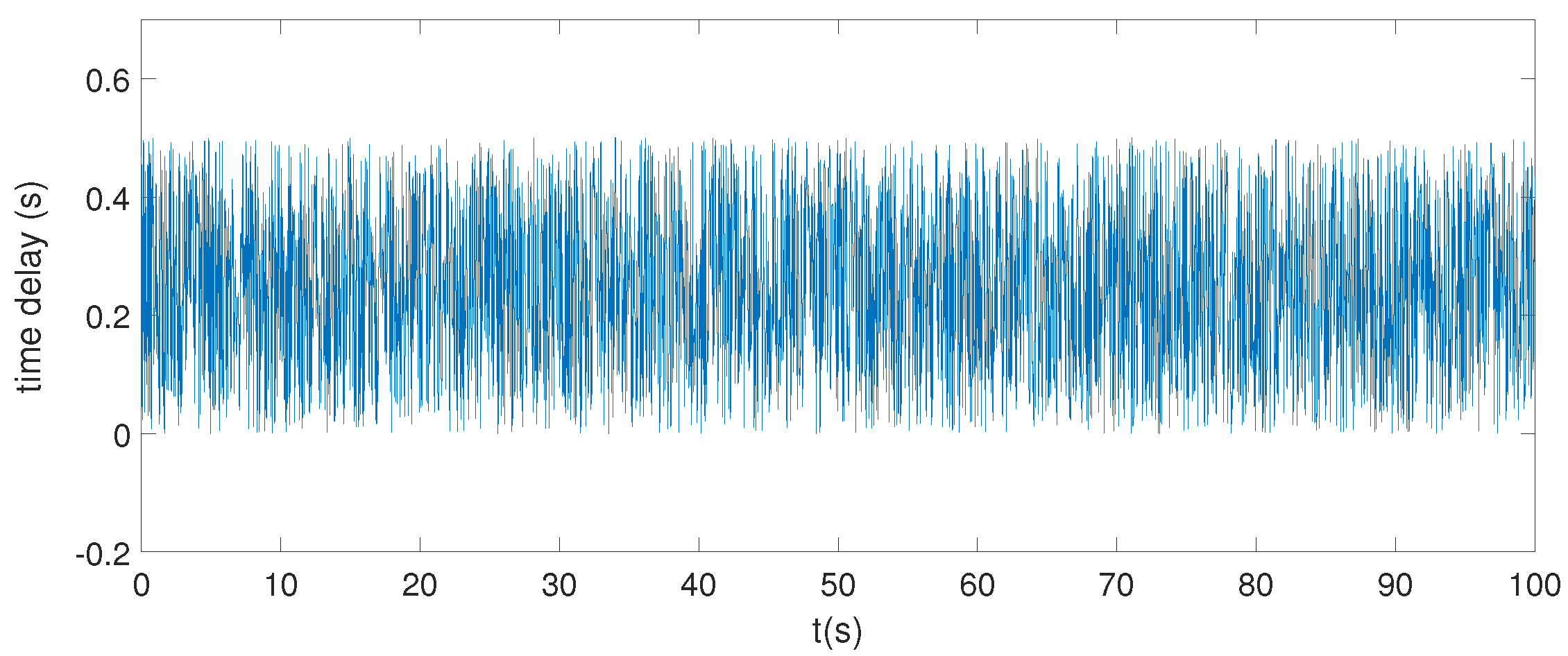
5. Simulations
6. Conclusions
Author Contributions
Funding
Conflicts of Interest
References
- Chen, Y.; Du, Z.; Garca-aacosta, M. Robot as a service in cloud computing. In Proceedings of the Fifth IEEE International Symposium on Service Oriented System Engineering, Nanjing, China, 4–5 June 2010; pp. 151–158. [Google Scholar]
- Ramírez De La Pinta, J.; Maestre Torreblanca, J.M.; Jurado, I.; Reyes De Cozar, S. Off the shelf cloud robotics for the smart home: Empowering a wireless robot through cloud computing. Sensors 2017, 17, 525. [Google Scholar] [CrossRef]
- Vega, J.; Cañas, J.M. PiBot: An open low-cost robotic platform with camera for STEM education. Electronics 2018, 7, 430. [Google Scholar] [CrossRef]
- Al-Wais, S.; Mohajerpoor, R.; Shanmugam, L.; Abdi, H.; Nahavandi, S. Improved delay-dependent stability criteria for telerobotic systems with time-varying delays. IEEE Trans. Syst. Man Cybern. Syst. 2017, 48, 2470–2484. [Google Scholar] [CrossRef]
- Sugiura, K.; Shiga, Y.; Kawai, H.; Misu, T. A cloud robotics approach towards dialogue-oriented robot speech. Adv. Robot. 2015, 29, 449–456. [Google Scholar] [CrossRef]
- Jahanshahi, H.; Jafarzadeh, M.; Sari, N.N.; Pham, V.-T.; Huynh, V.V.; Nguyen, X.Q. Robot motion planning in an unknown environment with danger space. Electronics 2019, 8, 201. [Google Scholar] [CrossRef]
- Ding, L.; Han, Q.L.; Zhang, X. Distributed secondary control for active power sharing and frequency regulation in islanded microgrids using an event-triggered communication mechanism. IEEE Trans. Ind. Inform. 2018. [Google Scholar] [CrossRef]
- Rabah, M.; Rohan, A.; Han, Y.-J.; Kim, S.-H. Design of fuzzy-PID controller for quadcopter trajectory-tracking. Int. J. Fuzzy Logic Intell. Syst. 2018, 18, 204–213. [Google Scholar] [CrossRef]
- Tiep, D.K.; Lee, K.; Im, D.-Y.; Kwak, B.; Ryoo, Y.-J. Design of fuzzy-PID controller for path tracking of mobile robot with differential drive. Int. J. Fuzzy Logic Intell. Syst. 2018, 18, 220–228. [Google Scholar] [CrossRef]
- Shahbazi, M.; Atashzar, S.F.; Tavakoli, M.; Patel, R.V. Position-force domain passivity of the human arm in telerobotic systems. IEEE/ASME Trans. Mechatron. 2018, 23, 552–562. [Google Scholar] [CrossRef]
- Santos, J.; Conceição, A.; Santos, T.; Araújo, H. Remote control of an omnidirectional mobile robot with time-varying delay and noise attenuation. Mechatronics 2018, 52, 7–21. [Google Scholar] [CrossRef]
- Li, W.; Liang, D.; Gao, H.; Tavakoli, M. Haptic tele-driving of wheeled mobile robots under nonideal wheel rolling, kinematic control and communication time delay. IEEE Trans. Syst. Man Cybern. Syst. 2017, 99, 1–12. [Google Scholar] [CrossRef]
- Farooq, U.; Gu, J.; El-Hawary, M.E.; Asad, M.U.; Abbas, G.; Luo, J. A time-delayed multi-master-single-slave non-linear tele-robotic system through state convergence. IEEE Access 2018, 6, 5447–5459. [Google Scholar] [CrossRef]
- Nuno, E.; Basanez, L.; Ortega, R. Passivity-based control for bilateral teleoperation: A tutorial. Automatica 2011, 47, 485–495. [Google Scholar] [CrossRef]
- Lee, J.; Chang, P.H.; Jin, M. Adaptive integral sliding mode control with time-delay estimation for robot manipulators. IEEE Trans. Ind. Electron. 2017, 64, 6796–6804. [Google Scholar] [CrossRef]
- Zhang, X.; Han, Q.; Ge, X.; Ding, D. An overview of recent developments in Lyapunov-Krasovskii functionals and stability criteria for recurrent neural networks with time-varying delays. Neurocomputing 2018, 313, 392–401. [Google Scholar] [CrossRef]
- Zhang, X.; Han, Q.; Wang, Z.; Zhang, B. Neuronal state estimation for neural networks with two additive time-varying delay components. IEEE Trans. Cybern. 2017, 47, 3184–3194. [Google Scholar] [CrossRef]
- Lian, H.; Xiao, S.; Wang, Z.; Zhang, X.; Xiao, H. Further results on sampled-data synchronization control for chaotic neural networks with actuator saturation. Neurocomputing 2019. [Google Scholar] [CrossRef]
- Yang, C.; Wang, X.; Li, Z.; Li, Y.; Su, C.-Y. Teleoperation control based on combination of wave variable and neural networks. IEEE Trans. Syst. Man Cybern. Syst. 2017, 47, 2125–2136. [Google Scholar] [CrossRef]
- Hua, C.; Liu, X.P. Teleoperation over the internet with/without velocity signal. IEEE Trans. Instrum. Meas. 2010, 60, 4–13. [Google Scholar] [CrossRef]
- Zhang, X.; Han, Q.; Seuret, A.; Gouaisbaut, F.; He, Y. Overview of recent advances in stability of linear systems with time-varying delays. IET Control Theory Appl. 2019, 13, 1–16. [Google Scholar] [CrossRef]
- Bowthorpe, M.; Tavakoli, M.; Becher, H.; Howe, R. Smith predictor-based robot control for ultrasound-guided teleoperated beating-heart surgery. IEEE J. Biomed. Health Inform. 2014, 18, 157–166. [Google Scholar] [CrossRef]
- Zhang, H.; Lu, X.; Cheng, D. Optimal estimation for continuous-time systems with delayed measurements. IEEE Trans. Autom. Control 2006, 51, 823–827. [Google Scholar] [CrossRef]
- Guechi, E.H.; Lauber, J.; Dambrine, M.; Defoort, M. Output feedback controller design of a unicycle-type mobile robot with delayed measurements. IET Control Theory Appl. 2012, 6, 726–733. [Google Scholar] [CrossRef]
- Lu, Z.; Huang, P.; Liu, Z. Predictive approach for sensorless bimanual teleoperation under random time delays with adaptive fuzzy control. IEEE Trans. Ind. Electron. 2018, 65, 2439–2448. [Google Scholar] [CrossRef]
- Efimov, D.; Fridman, E.; Polyakov, A.; Perruquetti, W.; Richard, J.-P. Linear interval observers under delayed measurements and delay-dependent positivity. Automatica 2016, 72, 123–130. [Google Scholar] [CrossRef]
- Ahmed-Ali, T.; Cherrier, E.; Lamnabhi-Lagarrigue, F. Cascade high gain predictors for a class of nonlinear systems. IEEE Trans. Autom. Control 2014, 57, 221–226. [Google Scholar] [CrossRef]
- Hernández, O.; Farza, M.; Ménard, T.; Targui, B.; M’Saad, M.; Astorga-Zaragoza, C.M. A cascade observer for a class of MIMO non uniformly observable systems with delayed sampled outputs. Syst. Control Lett. 2016, 98, 86–96. [Google Scholar] [CrossRef]
- Borhaug, E.; Pettersen, K.Y. Global output feedback PID control for n-DOF Euler–Lagrange systems. In Proceedings of the 2006 American Control Conference, Minneapolis, MN, USA, 14–16 June 2006; pp. 4993–4999. [Google Scholar]
- Erkan, Z.; Enver, T.; Egemen, K. A model independent observer based output feedback tracking controller for robotic manipulators with dynamical uncertainties. Robotica 2017, 35, 729–743. [Google Scholar]
- Sharma, N.; Bhasin, S.; Wang, Q.; Dixon, W.E. Predictor-based control for an uncertain Euler–Lagrange system with input delay. Automatica 2011, 47, 2332–2342. [Google Scholar] [CrossRef]
- Obuz, S.; Tatlicioglu, E.; Cekic, S.C.; Dawson, D.M. Predictor-based robust control of uncertain nonlinear systems subject to input delay. IFAC Proc. Vol. 2012, 45, 231–236. [Google Scholar] [CrossRef]
- Kamalapurkar, R.; Fischer, N.; Obuz, S.; Dixon, W.E. Time-varying input and state delay compensation for uncertain nonlinear systems. IEEE Trans. Autom. Control 2015, 61, 834–839. [Google Scholar] [CrossRef]
- Zhang, X.; Han, Q.; Zeng, Z. Hierarchical type stability criteria for delayed neural networks via canonical Bessel-Legendre inequalities. IEEE Trans. Cybern. 2018, 48, 1660–1671. [Google Scholar] [CrossRef] [PubMed]
- Wang, J.; Zhang, X.; Han, Q. Event-triggered generalized dissipativity filtering for neural networks with time-varying delays. IEEE Trans. Neural Netw. Learn. Syst. 2016, 27, 77–88. [Google Scholar] [CrossRef] [PubMed]
- Zhang, B.; Han, Q.; Zhang, X.; Yu, X. Sliding mode control with mixed current and delayed states for offshore steel jacket platform. IEEE Trans. Control Syst. Technol. 2014, 22, 1769–1783. [Google Scholar] [CrossRef]
- Su, Y.; Muller, P.C.; Zheng, C. A Simple Nonlinear observer for a class of uncertain mechanical systems. IEEE Trans. Autom. Control 2007, 52, 1340–1345. [Google Scholar]
- Zhou, L.; She, J.; Zhou, S.; Li, C. Compensation for state-dependent nonlinearity in a modified repetitive-control system. Int. J. Robust Nonlinear Control 2018, 28, 213–226. [Google Scholar] [CrossRef]
- Zhou, L.; She, J.; Zhou, S. Robust H∞ control of an observer-based repetitive-control system. J. Frankl. Inst. 2018, 355, 4952–4969. [Google Scholar] [CrossRef]


| K | |||||||
|---|---|---|---|---|---|---|---|
| 1 kg | 0.5 kg | 0.5 m | 0.5 m | 25 | 0.1 | 5 | 10 |
© 2019 by the authors. Licensee MDPI, Basel, Switzerland. This article is an open access article distributed under the terms and conditions of the Creative Commons Attribution (CC BY) license (http://creativecommons.org/licenses/by/4.0/).
Share and Cite
Shen, S.; Song, A.; Li, T. Predictor-Based Motion Tracking Control for Cloud Robotic Systems with Delayed Measurements. Electronics 2019, 8, 398. https://doi.org/10.3390/electronics8040398
Shen S, Song A, Li T. Predictor-Based Motion Tracking Control for Cloud Robotic Systems with Delayed Measurements. Electronics. 2019; 8(4):398. https://doi.org/10.3390/electronics8040398
Chicago/Turabian StyleShen, Shaobo, Aiguo Song, and Tao Li. 2019. "Predictor-Based Motion Tracking Control for Cloud Robotic Systems with Delayed Measurements" Electronics 8, no. 4: 398. https://doi.org/10.3390/electronics8040398