3D-MIMO Channel Estimation under Non-Gaussian Noise with Unknown PDF


School of Electronic and Information Engineering, Xi’an Jiaotong University, Xi’an 710049, China
*
Author to whom correspondence should be addressed.
Electronics 2019, 8(3), 316; https://doi.org/10.3390/electronics8030316
Submission received: 26 January 2019
/
Revised: 28 February 2019
/
Accepted: 7 March 2019
/
Published: 13 March 2019
(This article belongs to the Section Circuit and Signal Processing)
Abstract
:Three-dimensional-multiple-input-multiple-output (3D-MIMO) technology has attracted a lot of attention in the field of wireless communication. Most of the research mainly focuses on channel estimation model which is affected by additive-white-Gaussian-noise (AWGN). However, under the influence of some specified factors, such as electronic interference and man-made noise, the noise of the channel does not follow the Gaussian distribution anymore. Sometimes, the probability density function (PDF) of the noise is unknown at the receiver. Based on this reality, this paper tries to address the problem of channel estimation under non-Gaussian noise with unknown PDF. Firstly, the common support of angle domain channel matrix is estimated by compressed sensing (CS) reconstruction algorithm and a decision rule. Secondly, after modeling the received signal as a Gaussian mixture model (GMM), a data pruning algorithm is exerted to calculate the order of GMM. Lastly, an expectation maximization (EM) algorithm for linear regression is implemented to estimate the the channel matrix iteratively. Furthermore, sparsity, not only in the time domain, but in addition in the angle domain, is utilized to improve the channel estimation performance. The simulation results demonstrate the merits of the proposed algorithm compared with the traditional ones.
1. Introduction
The improvement of data transmission rate in wireless communication is of great meaning. Three-dimensional-multiple-input-multiple-output (3D-MIMO) can improve channel capacity without increasing the transmission power and bandwidth. Therefore, it has been one of the key technologies in the 5th-Generation communication systems. In addition, 3D-MIMO can enhance the spatial available dimension effectively compared with traditional MIMO by which only one horizontal dimension can be provided. Specifically, the traditional MIMO system has fewer ports that can only adjust the beam direction in the horizontal dimension, and cannot concentrate the vertical dimension energy on the receivers, while 3D-MIMO commonly used a two-dimensional antenna array in a large scale such as uniform planar array (UPA) [1] where hundreds of antennas can be placed in a small area. 3D-MIMO can flexibly adjust the direction of the beam in both the horizontal and vertical directions, forming a more precise and narrower directional beam, so as to enhance the received signal energy and strengthen the cell coverage greatly. Furthermore, 3D-MIMO can achieve the enhancement of spatial multi-user multiplexing capabilities and better interference suppression through the use of advanced signal processing technology. An important issue for 3D-MIMO utilization is to get the channel impulse response (CIR) accurately. However, with the conventional channel estimation method, massive multi-antenna means the sharp increase of pilot number [2], which is no longer proper for real application. Meanwhile, the MIMO channel is shown to have a specific sparse structure [3] in which the row and column vectors of the angular domain channel matrix are both sparse. Therefore, sparse estimation technology, such as compressed sensing (CS) based reconstruction algorithms, can be used to do channel estimation.
At the same time, most of the existing communication theory assumes that the noise at the receivers follows a Gaussian distribution [3,4,5]. These theories are mainly based on two reasons: (1) the Gaussian distribution can be expressed in specific mathematical expressions to facilitate analysis and calculation; (2) this assumption conforms to the central limit theorem. However, recent studies have shown that the noise is not always subjected to the Gaussian distribution in a lot of wireless applications [6,7,8]. If the noise is still be treated as a Gaussian distribution, it usually shows poor performance [9]. The reason for the non-Gaussian noise may be, for example, an atmospheric noise in radio links, lightning, relay contacts, ambient acoustic noise due to ice cracking in the arctic region in underwater sonar [8] and submarine communications [10,11]. Therefore, it is of great importance to address this problem in 3D-MIMO channel estimation.
A structured sparse channel estimation (SSCE) algorithm [12] has been studied to estimate a 3D-MIMO channel, but the influence of non-Gaussian noise needs to be studied further. The authors in [13] propose a channel estimation algorithm by refining the selection of dominant entries iteratively until the terminating condition is met but ignores the influence of non-Gaussian noise either. Meanwhile, channel estimation under non-Gaussian noise can be obtained by the method of the Kernel density, but the accuracy of which is seriously affected by the selection of kernel width [10]. In addition, the expectation maximization (EM) algorithm is regarded as an excellent way to solve the problem by modelling non-Gaussian noise as a Gaussian mixture model (GMM). However, most of the published works assume that the order of GMM is known previously [10,14,15], which is not always the case in real systems. Therefore, the order of GMM should be determined before the establishment of a mixture Gaussian function. This paper tries to address the order selection problem by a pruning approach.
On the other hand, the existence of sparsity of the 3D-MIMO channel matrix in the angular domain has been studied in [6], in which the channel matrix in the array domain is converted to the angular domain. In fact, as the distance of each antenna on the array are relatively close, the support set of all elements can be considered as the same [16]. Inspired by these works, this paper uses a CS-based reconstruction algorithm to estimate the common support of the angle domain channel matrix and obtain the sparse position of channel matrix firstly. Meanwhile, an order selection method is implemented in the determination of the order of GMM, which is used to approximate the real probability density function (PDF) of the noise. Finally, an EM algorithm for linear regression is used to estimate the channel support matrix.
The contribution of this paper is that it provides a framework of 3D-MIMO sparse channel estimation under non-Gaussian noise with unknown PDF.
The rest of this paper is organized as follows. In Section 2, the sparsity of 3D-MIMO channel matrix is presented. Section 3 gives the channel estimation algorithm under the environment of non-Gaussian noise, and the simulation proves the advantage of this method in Section 4. Section 5 provides the conclusions of this paper.
Notion: Let and denote transpose and Hermitian transpose, respectively; let ⊗ denote the Kronecker product; let represent a diagonal matrix with the value of vector in its diagonal; let and represent the absolute value and 2-norm operation respectively; and let indicate the circularly symmetric complex Gaussian random vector with mean and covariance matrix . Its expression for a d-dimensional vector of is
2. System Model
2.1. Signal Model
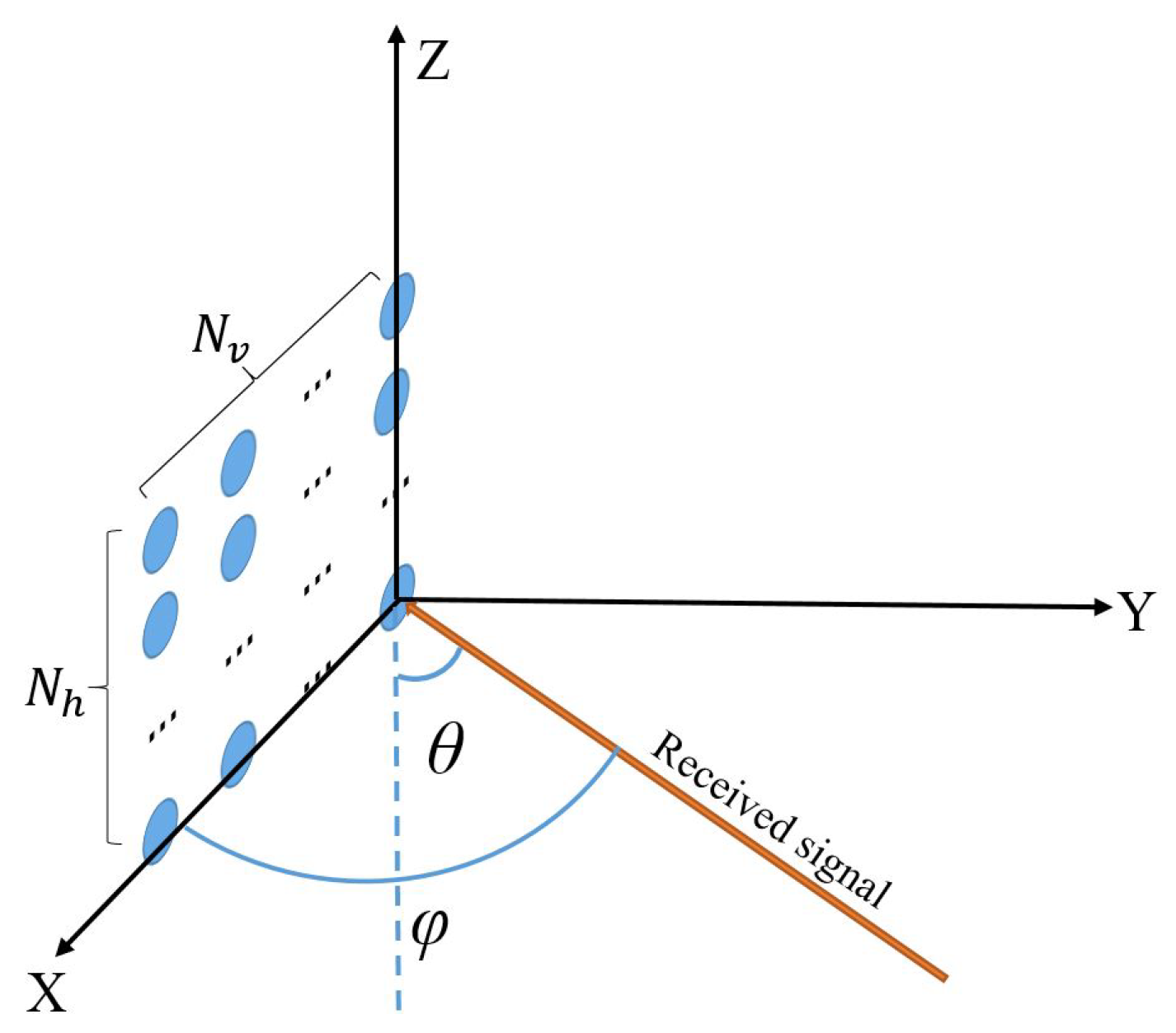
Consider an orthogonal frequency division multiplexing access uplink cellular system with K users in a cell. Each user has one transmission antenna. The K users are randomly distributed in the cell. The UPA is installed in the base station which holds elements in a vertical direction and in a horizontal direction, and is the total number of antennas. The antenna model of the base station is illustrated in Figure 1. According to [17], the CIR for the k-th user in matrix form can be expressed as
where P is the total number of multipaths of this user. In addition, denotes the fading coefficient. Furthermore, and denote the steering vector in the vertical direction and horizontal direction, respectively, and they can be expressed as
where
In addition, and represent the pitch direction of arrival (DoA) and azimuth DoA, respectively, for the l-th path as shown in Figure 1, and represent the minimum distance in the row and column of the adjacent element on the UPA, respectively, and is the wavelength of the signal. The channel matrix can be rewritten in array domain form as
where is the vector form of the channel of the i-th path of user k, which can be written as
Transforming the channel matrix of the k-th user in Equation (4) from an array domain into angle domain yields
where is the conjugation of Kronecker product of spatial base vector, and and express the mutually independent spatial horizontal base vector and vertical base vector, respectively. These base vectors can be expressed as
After transmission, the received signal at the base station can be written as
where is the received signal, is the gather of the pilot signals, is the dimension of the pilot vector, and
is the channel matrix of all users. The pilot vector set is
where is the pilot vector sent by user i, and it is a dimensional column vector. In addition, is composed by K matrix that is on the diagonal of , where is the first P columns of dimensional Fourier transform matrix with
where and . According to Equation (6), the received signal can be transformed from array domain into angle domain as shown in Equation (11),
where is a known dimensional transmission matrix with elements , , , and that represent , , and angular domain transformed matrixes, respectively. The goal of channel estimation is to obtain from the known matrix and under non-Gaussian noise .
2.2. Description of Joint Sparsity of Angle Domain Channel Matrix
The joint sparsity of 3D-MIMO angle domain channel matrix can be used to improve the channel estimation performance. As a matter of fact, the sparsity of the channel matrix does not only lie in the time domain, but also in the angle domain, which results in the sparsity both in columns and rows of angle domain channel matrix.
2.2.1. The Sparsity of the Column Vector
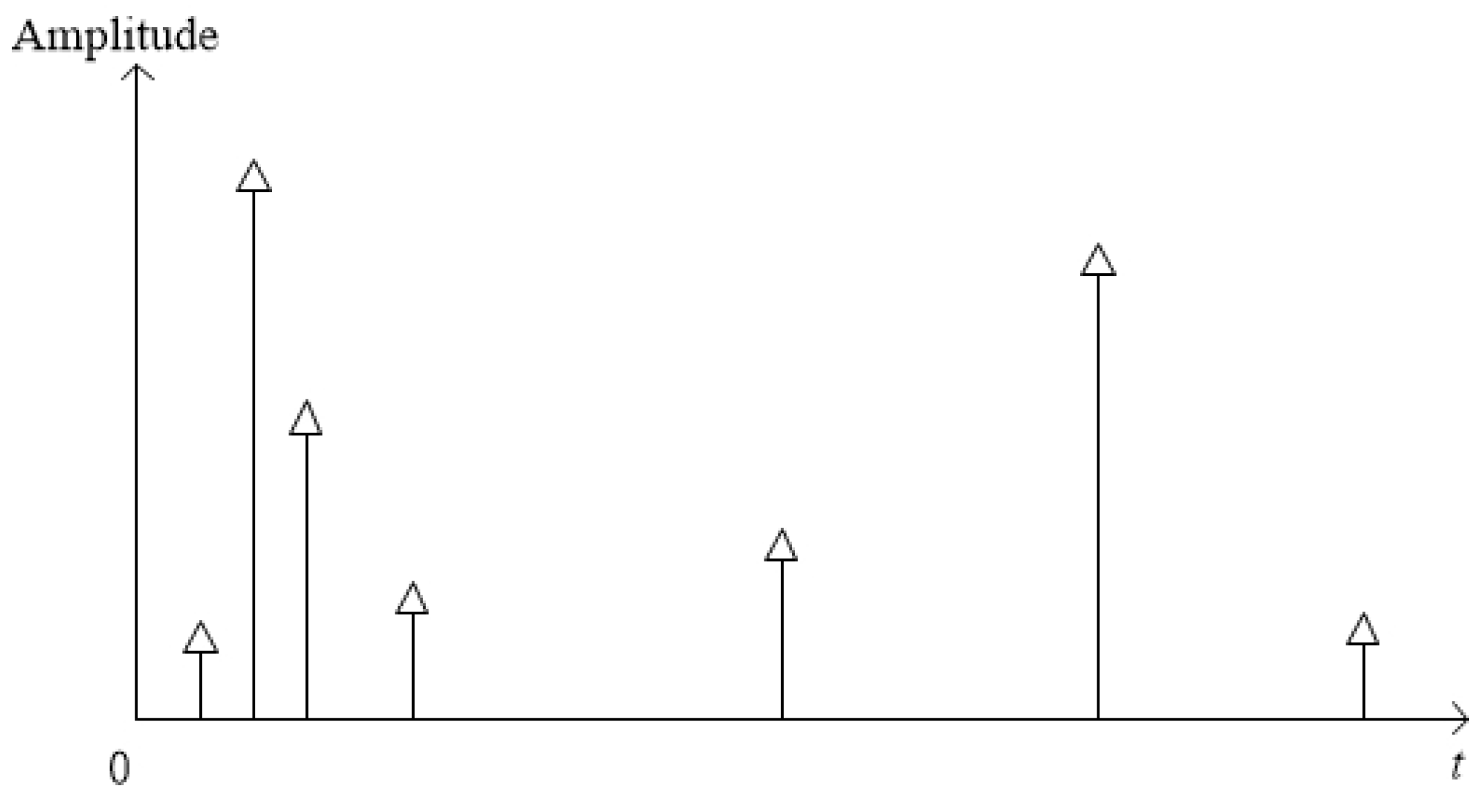
Due to the existence of multipath effect and transmission delay, the arrival time of the same transmitted signal transmission from the transmitter to the receiver is different from each other, as shown in Figure 2. That is to say, the receiver will receive the duplicates of the transmitted signals at different times. In real systems, there is hardly any signal arrives at most of the times during this period. The elements of a column of angle domain channel matrix represent the intensity of arrived signal from the transmitters through all of the paths for a corresponding antenna element in UPA. Therefore, the sparsity in the time domain results in the sparsity of the column vector.
2.2.2. The Sparsity of the Row Vector
The sparsity of the row vector is caused by the scatters around the base station. The uplink transmitted signals can be received by a small fraction of spatial reign of the base station because the location of the base station is generally high enough [12]. In addition, the signal arrives at the receivers only in some particular angle bin, which leads to the sparsity of transmitted signals in the angle domain [3]. Furthermore, it has been demonstrated in [16] that all of the antennas share a common support if the distance among the farther antennas of the UPA satisfies the following condition:
where c is the speed of light, and is the bandwidth of transmitted signal. In general, conforms to such a joint sparsity: its row vectors and column vectors are both sparse, and all of the column vectors have the same position.
3. Channel Estimation under Non-Gaussian Noise
This section proposes a channel estimation algorithm when the noise does not follow Gaussian distribution, and the PDF is unknown either.
In summary, the proposed algorithm estimates the angle domain channel matrix through three steps:
- (1)
- Estimate the common support to obtain the sparse position;
- (2)
- Approximate the unknown PDF of the noise using mixture Gaussian function;
- (3)
- Estimate angle domain channel matrix by linear regression EM algorithms.
3.1. The Estimation of the Common Support
To get the common support, a CS reconstruction algorithm is implemented to coarsely estimate angle domain channel matrix, and then the common support of angle domain channel matrix is obtained directed by a decision rule. After applying Equation (11) to CS algorithms, we can preliminarily get the estimation of angle domain channel matrix written as . Then, the common support is denoted as
with
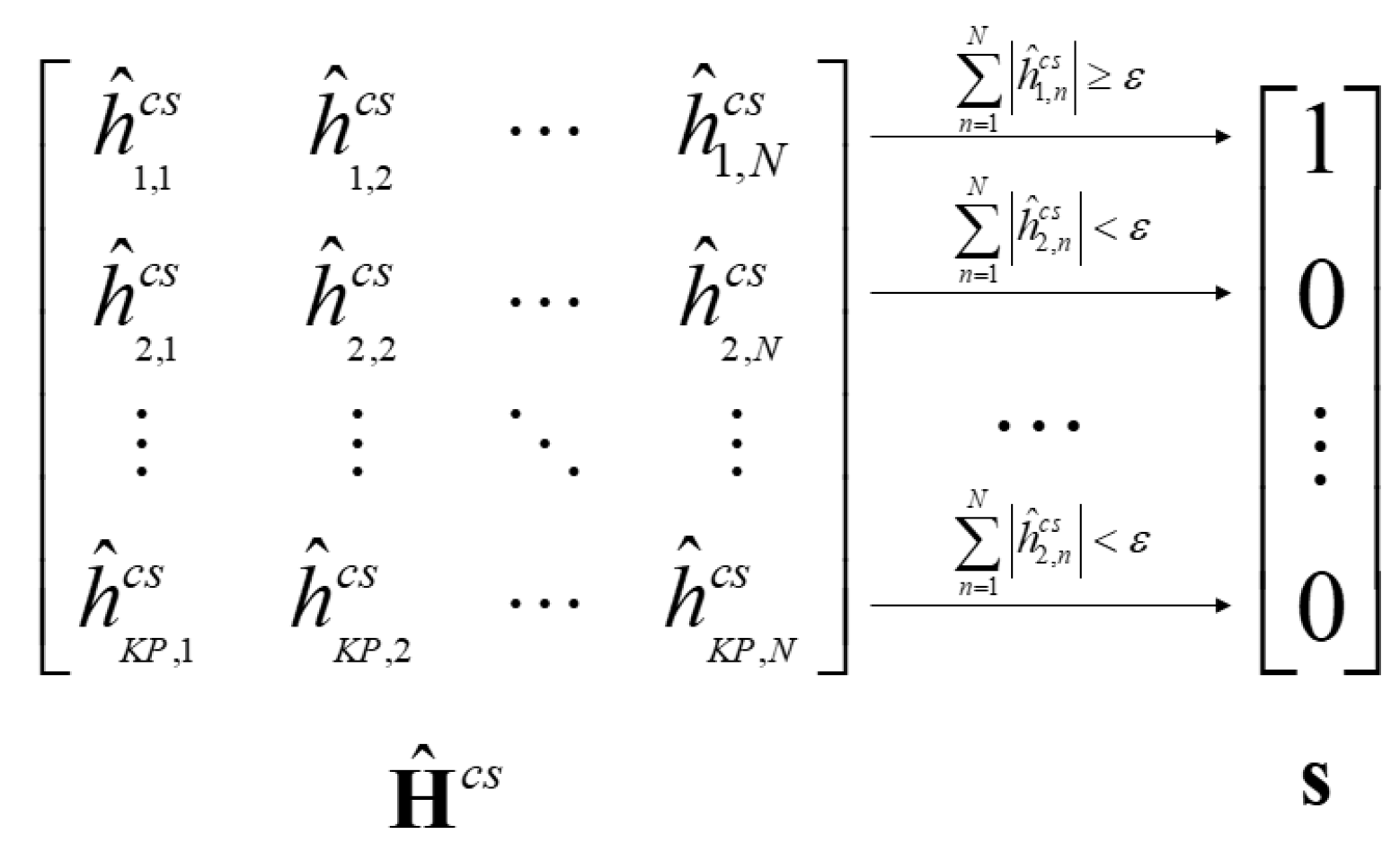
where is the i-th element of , and is the threshold to judge the value of the common support. In fact, is related to the signal to noise ratio (SNR) of the receivers. The value should be chosen properly; otherwise, it will lead to an inaccurate estimation of sparse positions and channel estimation. Furthermore, in Equation (13),
is the sum of the absolute value of the i-th row in , and is the element of in the i-th row and the n-th column. The i-th element in is 1 or 0 when the sum of absolute values of the i-th row in is larger or smaller than the threshold , respectively. Figure 3 gives the detailed conversion relationship between and .
Since the column of is sparse, most of its row vectors are the zero vector. The removal of these row vectors can save the computational cost and improve the speed of channel estimation without affecting the value of the received signal. In order to conduct the matrix multiplication operation correctly, the column vectors of at the corresponding positions should also be removed. In other words, the computational cost can be saved by reducing the dimension of and . After dimension reduction operation, the transmission support matrix is a submatrix generated by picking up the column of the transmission matrix , whose column index corresponds to the element 1 in .
3.2. Order Selection
In order to obtain the channel matrix, the PDF of the noise should be cognised firstly. Inspired by [18], the PDF of the unknown noise can be modeled as GMM with zero mean written as
where the parameter is the coefficient of component i, with
for mixture distribution components, is the covariance matrix for the i-th component, and is the order of GMM. Based on Equation (14), the noise cognition process can be transformed to the estimation of the key parameters and .
It should be noted that the order in the classical algorithm is assumed to be known, and it is always chosen from 2 to 4. This assumption is reasonable in the case of a specific non-Gaussian noise. Take impulse noise as an example, in the step of establishing its PDF by GMM, the mainstream approach is to select the order as 2 [19,20], and the results of this supposition are usually satisfactory. However, for more complicated non-Gaussian noise and interference model in real systems, order 2 to 4 may not be appropriate enough. In fact, when the number of the components is not large enough, the mixture model may underfit the data and may not be flexible enough to approximate the true noise. On the other hand, it may overfit the data and yield poor interpretations with too many components. Therefore, in order to describe the unknown distribution using GMM, the proper order should be studied at this step.
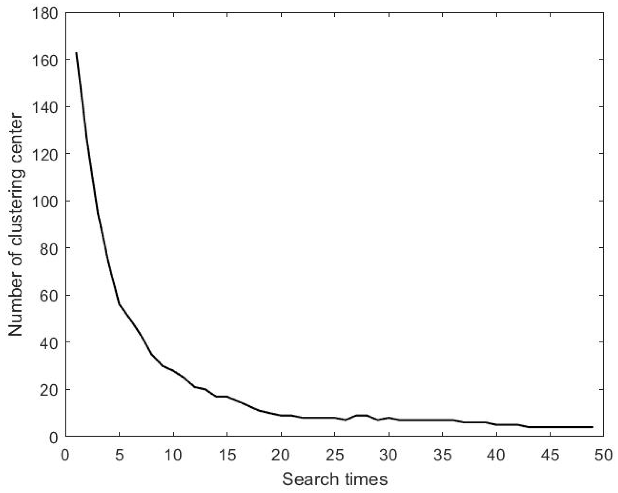
Inspired by the pruning algorithm in [21], this paper tries to propose an improved approach to determine the order of GMM. The main idea of the algorithm in [21] is implemented by an iterative manner. After each iteration, a clustering center of the data set is found, and then some data is deleted from the total data set according to this clustering center. Until all of the data has been deleted completely, the iteration is terminated. After the iteration is completed, the number of the clustering center represents the order of GMM. At each iterative step, the clustering centers are determined by the number of data in the neighborhood of a given radius. With the increase of radius, the number of the clustering center will decrease, which leads to different results of cluster numbers. However, the radius of a certain range will lead to the same number and location of the center points. The search procedure is terminated and the order is obtained when one state sustains more than M times.
However, in the communication systems, the characteristics of the Gaussian components of GMM are not always obvious. Under these circumstances, the method mentioned above needs to be improved. Specifically, when the Gaussian components are similar to each other, this method may take the clustering center center points as a cluster, with each point on the edge as a new one, even if there is only one point left in this cluster. This will lead to a large number of clusters, of which the result is unsatisfactory for the order selection. In order to overcome this problem, this paper proposes an improvement measure. In particular, after finding each clustering center and deleting this cluster of points, the variance of the remaining points is calculated. If the variance is smaller than the threshold , the next clustering center will be searched sequentially. Otherwise, the remaining points will be abandoned, and then the neighborhood radius is increased in the next step. Figure 4 illustrates the steps of the proposed method. Therefore, after setting the initial neighborhood radius, the proposed algorithm then gradually increases radius to search for the center cluster point.
The initial radius is set to be
where r is the initial radius, and are arbitrary elements of the data set, and the parameter R is used to control the search accuracy. The larger the parameter R is, the more accurate the result is, while the calculation complexity increases. This order reduction process is shown in Figure 4 and Figure 5.
3.3. Estimation of Channel Support Matrix
In this section, we will use the received signal and transmission support matrix to estimate the channel support matrix under the influence of non-Gaussian noise with independent and identically distributed components with PDF approximated by Equation (1). Without loss of generality, the mean of channel noise is assumed to be in Equation (14). In order to estimate the channel support matrix, instead of solving the linear regression problem in vector form in [19], this paper proposes to make an extension by transforming it into the matrix form. Furthermore, after the order has been obtained at the step of order selection, the channel support matrix can be calculated column by column. For the i-th column, its elements and the weight value least squares matrix can be calculated iteratively. Before the start of the algorithm, the i-th column vector of channel support matrix, coefficients and variances should be given initial values. The calculation process of is to perform Equations (16)–(18) one after another:
In Equation (16), is the prior probability of the k-th component, , , is the element of in the n-th row and the i-th column, is the element of in the n-th row and the m-th column, is the m-th element in , the superscript t is the number of iteration, and and are coefficients and variances of the k-th component of GMM.
The i-th column of channel matrix and its parameters of each component of GMM can be deducted based on and as
Repeat Equation (16)–(21) for all of the other columns, the whole channel support matrix can be obtained by
The iteration is terminated when the estimation value of channel support matrix is relatively stable or the given number of iterations has been done. This condition can be written in Equation (23) as
In (23), m is the total number of the 1 elements in , is the threshold, and is the given number of iteration number. After the iteration is completed, the final angle domain channel matrix can be achieved based on the channel support matrix and common support .
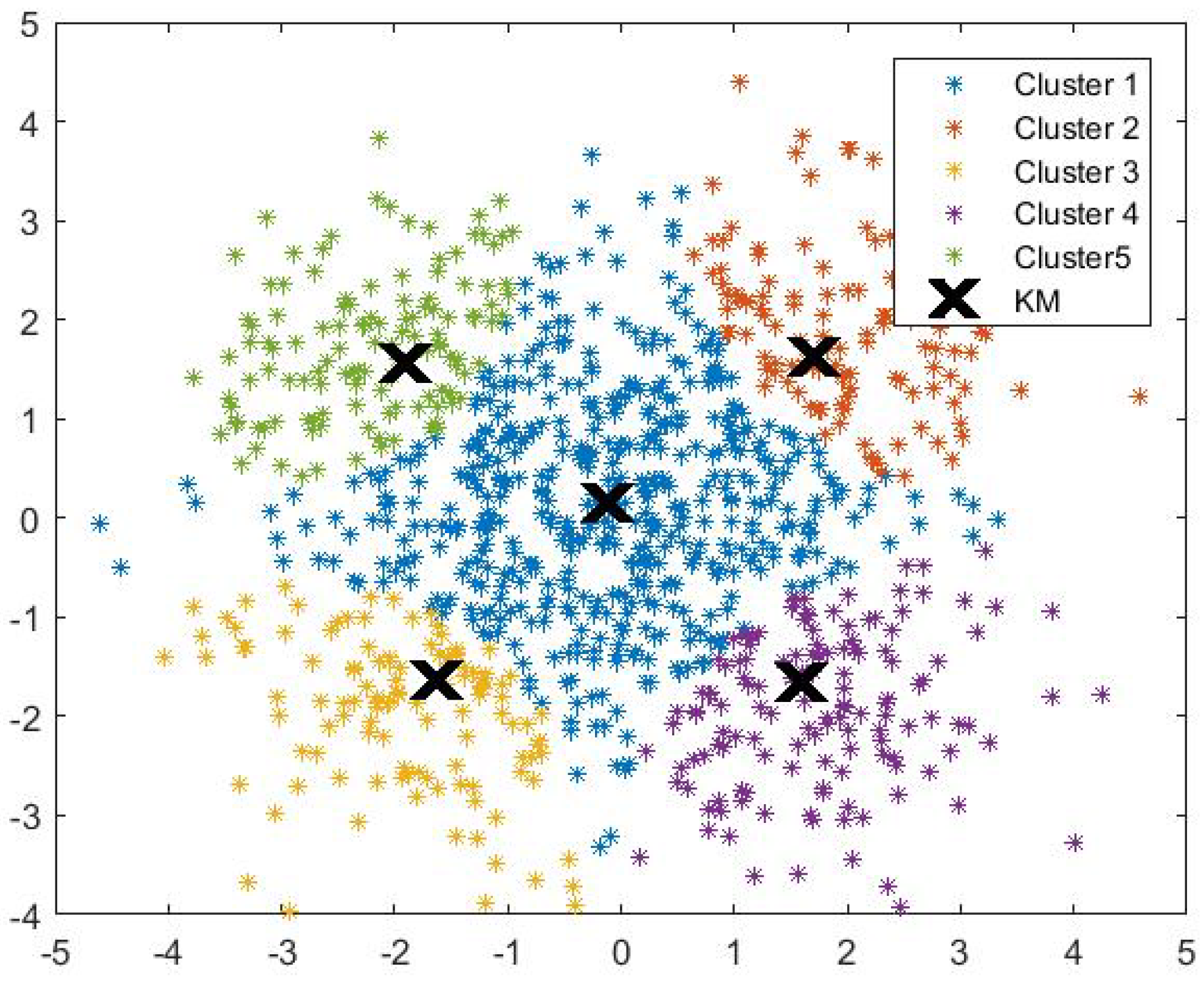
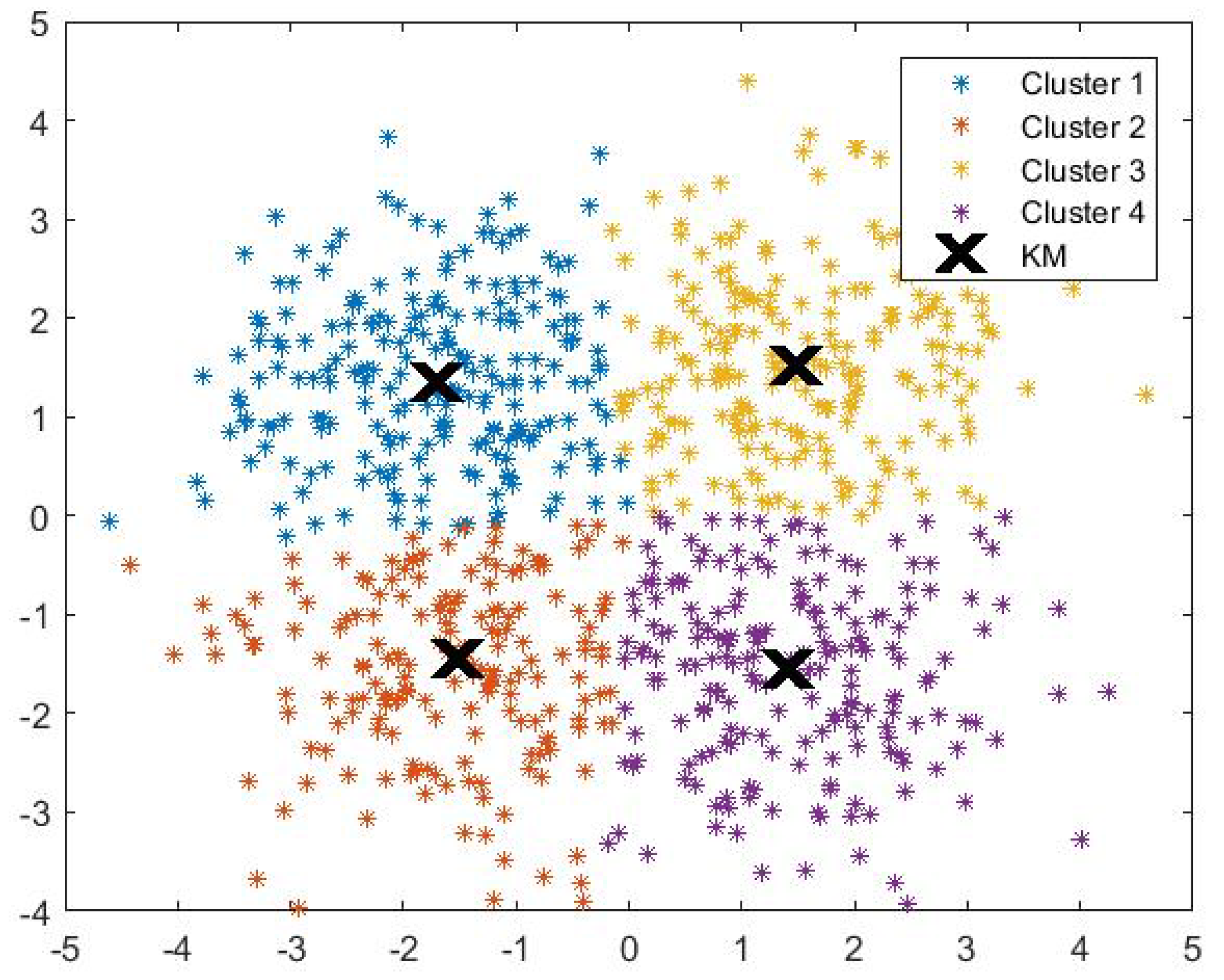
The reason for common support estimation going before order selection is that a large number of vectors which are 0 or close to 0 have a great impact on the accuracy of estimation of the order of GMM. For example, Figure 6 and Figure 7 show the result of order selection before and after removing the elements which are close to 0, respectively. In Figure 6, due to the presence of large number of elements which are close to 0 s, these elements will automatically generate a new class, so its clustering result is bigger than the data of Figure 7.
The main steps of the above algorithm are summarized in Algorithm 1.
| Algorithm 1 Non-Gaussian Angular Domain Sparse Channel Estimation |
| Input: received signal , transmission matrix , iterative counter , threshold: , M, R, , , Output: channel matrix
|
4. Simulation
This section demonstrates the simulation results. The frequency selective multipath channel consists of 200 independent Rayleigh multipath with maximum delay spread of s. The total transmission power is 1 W, the number of subcarriers is 2048, and the total transmission bandwidth is 8 MHz. The power delay is assumed to be an exponentially decaying profile. In the simulation process, the channel noise follows a mixture Gaussian distribution. The simulation parameters are shown in Table 1.
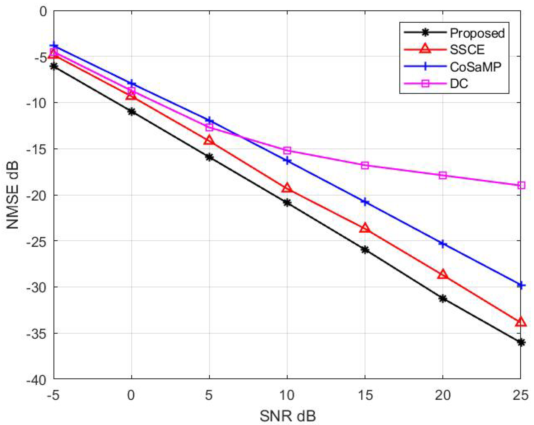
Figure 8 shows the comparison between the proposed algorithm and other three algorithms in aspect of the normalized mean square error (NMSE) over SNR, including an SSCE-based [12] algorithm, compressive sampling matching pursuit (CoSaMP) [22] sparse recovery algorithm, and the dual crossing (DC) algorithm [13]. From Figure 8, it can be seen that the SSCE algorithm has a comparatively satisfactory performance under Gaussian noise, especially in a relatively low SNR region. However, under the affect of non-Gaussian noise, its performance is not as good as the proposed method, which is reflected in Figure 8. It should be noted that, when the order of GMM is = 1, in other words, the noise follows Gaussian distribution, the proposed algorithm is similar to SSCE algorithm. The CoSaMP algorithm which has been used at the step of estimating the support set estimates the channel matrix based on classical CS reconstruction algorithm with the noise distribution being viewed as Gaussian distribution. In fact, the reconstruction performance of CoSaMP outperforms the other CS algorithms. Therefore, it is reasonable to use the CoSaMP algorithm as a reconstruction approach to estimate the support set at step 2 of Algorithm 1. The DC-based algorithm estimates channel by refining the selection of dominant entries iteratively until the terminating condition is met. It can also be seen from Figure 8 that the NMSE of the proposed algorithm is obviously superior to the traditional CoSaMP-based algorithm, SSCE-based algorithm and DC-bases algorithm. For example, when the SNR is 10 dB, the NMSE of the proposed algorithm is about −21 dB, and the traditional algorithm of SSCE-based, CoSaMP-based and DC-based is about −19 dB, −17 dB and −15 dB, respectively. When the SNR is 15 dB, the NMSE of the proposed algorithm, CoSaMP-based algorithm, SSCE-based algorithm and the DC-based algorithm is about −26 dB, −23 dB, −21 dB and −17 dB, respectively, thus the proposed algorithm has approximately 13.0%, 23.8%, and 52.9% improvement in terms of NMSE compared with traditional SSCE-based, CoSaMP-based, and DC-based, respectively.
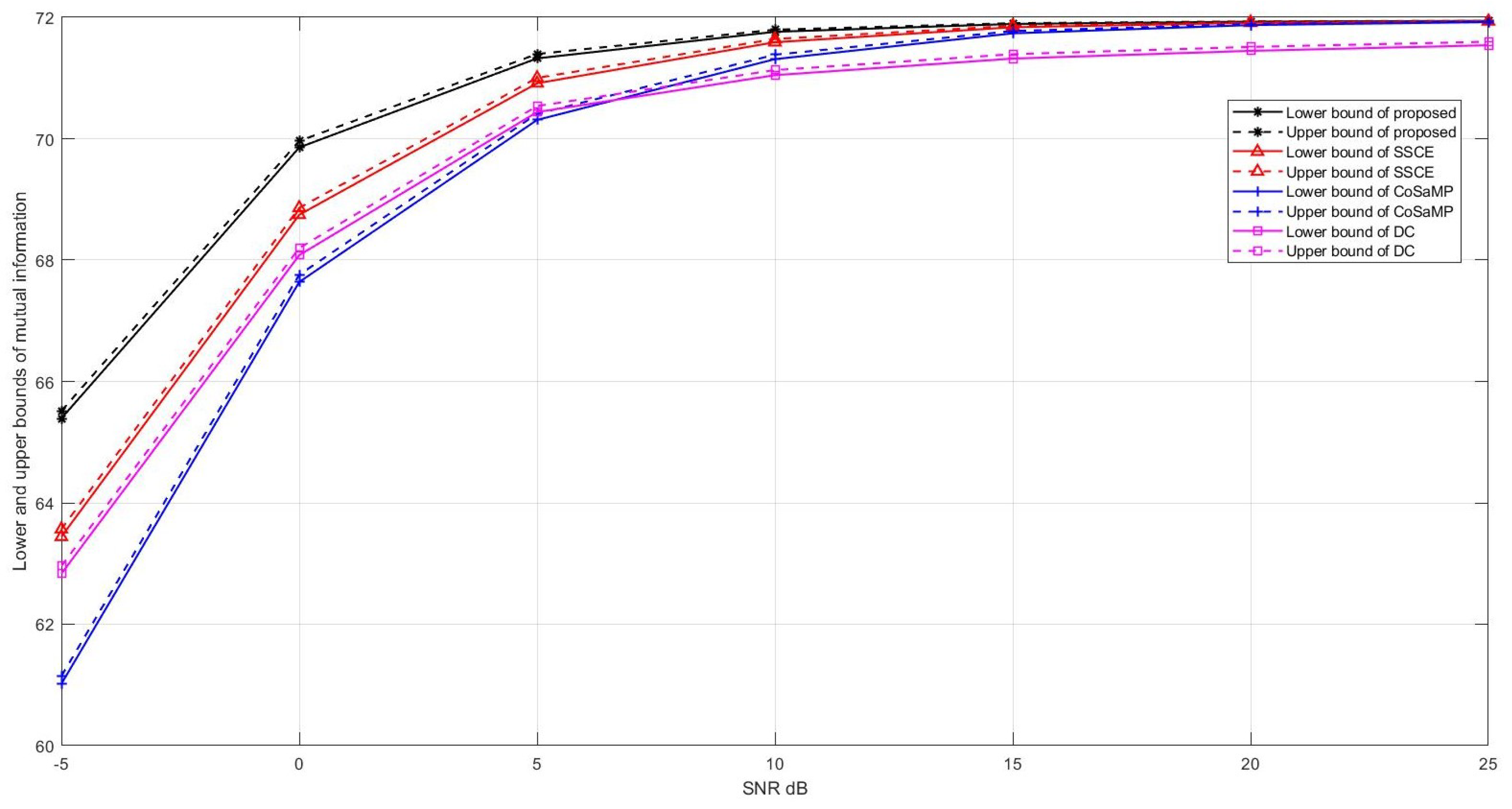
Imperfect channel state information (CSI) can cause the reduction of channel capacity [23]. Furthermore, if the CSI of the receiver is not perfect, the channel capacity will decrease significantly [24]. However, to the best of our knowledge, there is no precise mathematical relationship between the estimation error of CSI and the channel capacity for a MIMO system, which is still an open problem in the field of information theory. Fortunately, as mentioned in [25], the upper and lower bounds of mutual information can be determined according to channel estimation error. Based on [25], Figure 9 shows the comparison of the upper and lower bounds of mutual information between the proposed algorithm and other traditional algorithms versus SNR. It can be seen from this figure that the mutual information of the proposed algorithm is bigger than the mutual information of the traditional channel estimation algorithms when the SNR is relatively small. The difference becomes smaller when the SNR is relatively large because the channel estimation of all of the algorithms becomes more accurate and the NMSE of all of the algorithms becomes smaller.
The relationship between the number of antennas and the NMSE is shown in Figure 10. In the simulation of this figure, the pilot length is set to 512. For a given number of the pilots, the estimated error of the channel matrix increases as the number of antennas. In addition, it can be seen that when the number of antennas increases, the slope of the curves becomes smaller.
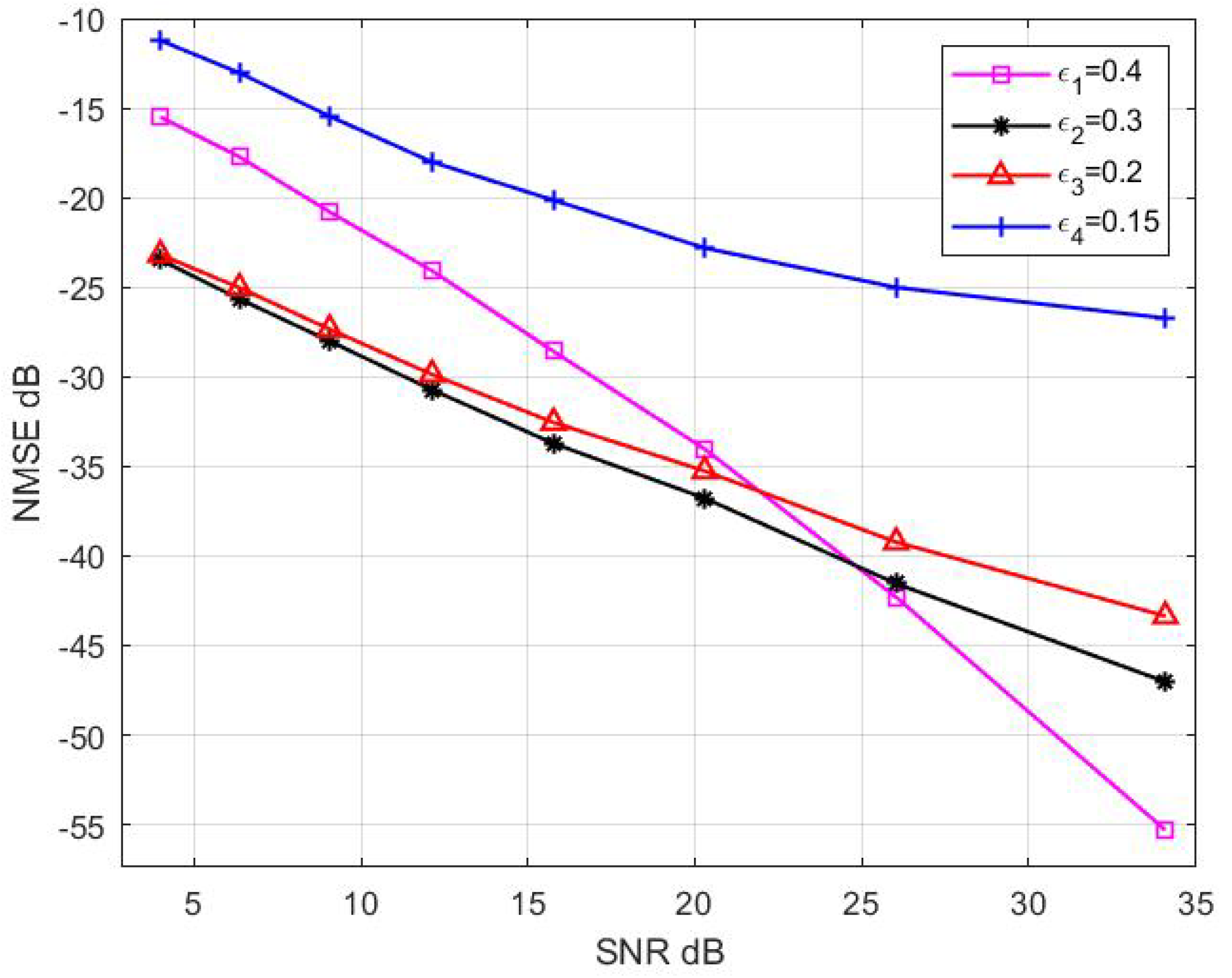
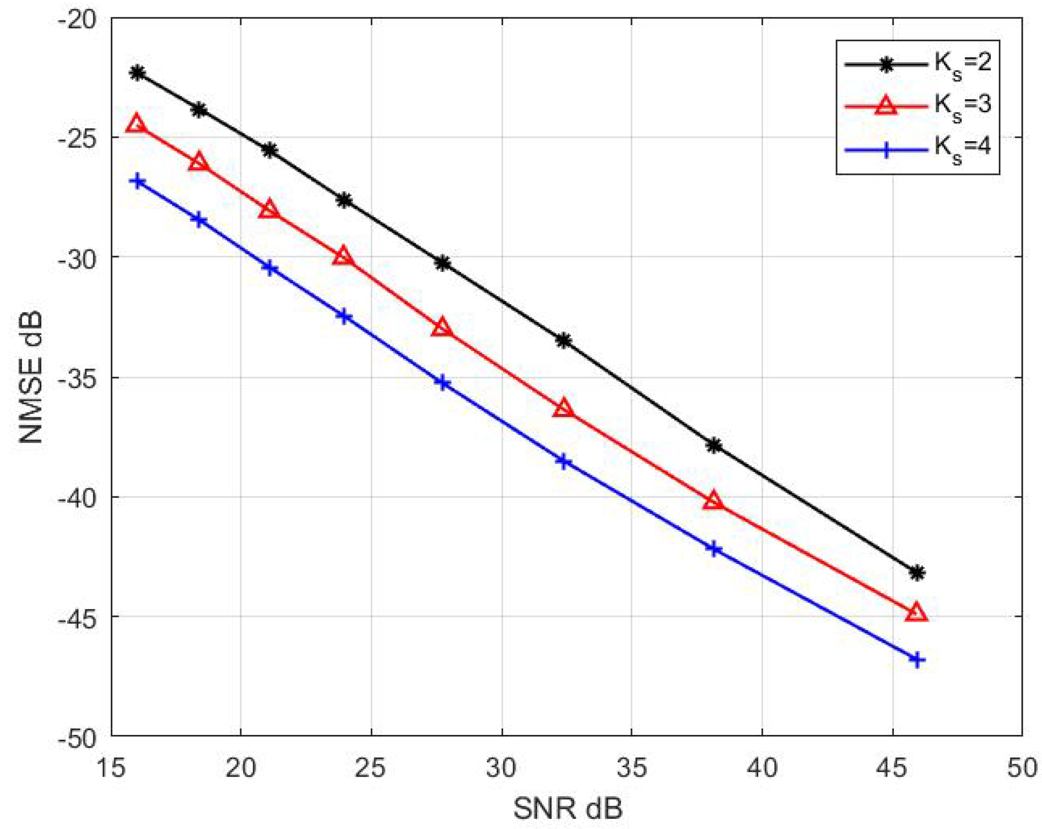
Figure 11 shows the impact of the value of on the results. According to the theoretical analysis, the value of is closely related to the received SNR. When the SNR is large, the value of can be chosen from a relative large range, and vice versa. Figure 12 demonstrates the effect of the choice of order of GMM on the performance channel estimation. In the simulation process, the channel noise is set to follow a GMM with order 4. It can been seen that the Gaussian mixture model with order 4 is superior to orders 2 or 3, which is not correctly estimated. For example, when the NMSE is −40 dB, the SNR gap is about 2.75 dB and 6.15 dB over orders 3 and 2, respectively. Therefore, choosing the appropriate GMM order is important for the system performance.
5. Conclusions
This paper studies a new algorithm that exploits the sparsity of 3D-MIMO in both time and angular domain to estimate channel matrix under non-Gaussian noise with unknown PDF. The core of the proposed algorithm is to recognize the noise by approximating the unknown PDF with GMM, and the order of GMM is also calculated after the estimation of the common support set of the channel matrix in the angle domain. After that, the channel support matrix is estimated under non-Gaussian noise. The proposed algorithm studies the property of the noise firstly and then estimates the CIR targeted on it; therefore, it outperforms the traditional approaches which view the noise distribution as Gaussian. Theoretical analysis and simulations show that the proposed algorithm is an effective method to solve the channel estimation problem under non-Gaussian noise for 3D-MIMO systems.
Author Contributions
Conceptualization, W.C., F.L. and Y.P.; methodology, W.C. and F.L.; software, W.C.; validation, W.C.; writing—original draft preparation, W.C.; writing—review and editing, W.C. and F.L.; supervision, F.L.; project administration, F.L.; funding acquisition, F.L.; Y.P. provided some technical comments.
Funding
This research received no external funding.
Conflicts of Interest
The authors declare no conflict of interest.
References
- Zhang, Y.; Zhang, R.; Lu, S.; Duan, W.; Cai, L. Measurement and modeling of indoor channels in elevation domain for 3D MIMO applications. In Proceedings of the IEEE International Conference on Communications (ICC), Sydney, Australia, 10–14 June 2014; pp. 659–664. [Google Scholar]
- Rao, X.; Lau, V. Distributed compressive CSIT estimation and feedback for FDD multi-user massive MIMO systems. IEEE Trans. Signal Process. 2014, 62, 3261–3271. [Google Scholar] [CrossRef]
- Bajwa, W.; Haupt, J.; Sayeed, A.; Nowak, R. Compressed channel sensing: A new approach to estimating sparse multipath channels. Proc. IEEE 2010, 98, 1058–1076. [Google Scholar] [CrossRef]
- Berger, C.; Wang, Z.; Huang, J.; Zhou, S. Application of compressive sensing to sparse channel estimation. IEEE Commun. Mag. 2010, 48, 164–174. [Google Scholar] [CrossRef]
- Hespanha, J.; Naghshtabrizi, P.; Xu, Y. A survey of recent results in networked control systems. Proc. IEEE 2007, 95, 138–162. [Google Scholar] [CrossRef]
- Zhang, Y.; Blum, R. An adaptive receiver with an antenna array for channels with correlated non-Gaussian interference and noise using the SAGE algorithm. IEEE Trans. Signal Process. 2010, 48, 2172–2175. [Google Scholar] [CrossRef]
- Zhao, X.; Li, F. Sparse bayesian compressed spectrum sensing under Gaussian mixture noise. IEEE Trans. Veh. Technol. 2018, 67, 6087–6097. [Google Scholar] [CrossRef]
- Sha’ameri, A.Z.; Al-Aboosi, Y.Y.; Khamis, N.H.H. Underwater acoustic noise characteristics of shallow water in tropical seas. In Proceedings of the 2014 International Conference on Computer and Communication Engineering, Kuala Lumpur, Malaysia, 23–24 September 2014; pp. 80–83. [Google Scholar]
- Kozick, R.J.; Sadler, B.M. Maximum-likelihood array processing in non-Gaussian noise with Gaussian mixtures. IEEE Trans. Signal Process. 2000, 48, 3520–3535. [Google Scholar] [CrossRef]
- Bhatia, V.; Mulgrew, B. Non-parametric likelihood based channel estimator for Gaussian mixture noise. Signal Process. 2007, 87, 2569–2586. [Google Scholar] [CrossRef]
- Tsihrintzis, G.; Nikias, C. Performance of optimum and suboptimum receivers in the presence of impulsive noise modeled as an alpha-stable process. IEEE Trans. Commun. 1995, 43, 904–914. [Google Scholar] [CrossRef]
- Liu, K.; Feng, H.; Yang, T.; Hu, B. Structured sparse channel estimation for 3D-MIMO systems. In Proceedings of the IEEE Vehicular Technology Conference (VTC Spring), Nanjing, China, 15–18 May 2016; pp. 1–6. [Google Scholar]
- Ma, W.; Qi, C. Channel Estimation for 3D Lens Millimeter Wave Massive MIMO System. IEEE Commun. Lett. 2017, 21, 2045–2048. [Google Scholar] [CrossRef]
- Zhang, Y.; Blum, R. An adaptive spatial diversity receiver for correlated non-Gaussian interference and noise. In Proceedings of the Asilomar Conference on Signals, Systems and Computers, Pacific Grove, CA, USA, 1–4 November 1998; pp. 1428–1432. [Google Scholar]
- Zamiri, H.; Pasupathy, S. EM-based recursive estimation of channel parameters. IEEE Trans. Commun. 1999, 47, 1297–1302. [Google Scholar] [CrossRef]
- Barbotin, Y.; Hormati, A.; Rangan, S.; Vetterli, M. Estimation of sparse MIMO channels with common support. IEEE Trans. Commun. 2012, 60, 3705–3716. [Google Scholar] [CrossRef]
- Feng, H.; Zhang, S.; Liu, K.; Hu, B.; Yang, T. From Sparse Channel to Sparse Beamforming: A 3D-MIMO case. In Proceedings of the IEEE Global Communications Conference, San Diego, CA, USA, 6–10 December 2015; pp. 1–6. [Google Scholar]
- Campbell, W.; Sturim, D.; Reynolds, D. Support vector machines using GMM supervectors for speaker verification. IEEE Signal Process. Lett. 2006, 13, 308–311. [Google Scholar] [CrossRef]
- Kozick, R.; Blum, R.; Sadler, B. Signal processing in non-Gaussian noise using mixture distributions and the EM algorithm. In Proceedings of the Asilomar Conference on Signals, Systems and Computers, Pacific Grove, CA, USA, 2–5 November 1997; pp. 438–442. [Google Scholar]
- Portilla, J.; Strela, V.; Wainwright, M.; Simoncelli, E.P. Image denoising using scale mixtures of Gaussians in the wavelet domain. IEEE Trans. Image Process. 2003, 12, 1338–1351. [Google Scholar] [CrossRef] [PubMed]
- Zhu, Y.; Ma, J. A stage by stage pruning algorithm for detecting the number of clusters in a dataset. In Proceedings of the International Conference on Intelligent Computing, Changsha, China, 18–21 August 2010; pp. 222–229. [Google Scholar]
- Needell, D.; Tropp, J. CoSaMP: Iterative signal recovery from incomplete and inaccurate samples. Appl. Comput. Harmon. Anal. 2009, 26, 301–321. [Google Scholar] [CrossRef] [Green Version]
- Goldsmith, A. Wireless Communications; Cambridge University Press: Cambridge, UK, 2005. [Google Scholar]
- Lapidoth, A.; Shamai, S. Fading channels: How perfect need “perfect side information” be? In Proceedings of the 1999 IEEE Information Theory and Communications Workshop (Cat. No. 99EX253), Kruger National Park, South Africa, 20–25 June 1999; pp. 36–38. [Google Scholar]
- Yoo, T.; Goldsmith, A. Capacity and power allocation for fading MIMO channels with channel estimation error. IEEE Trans. Inform. Theory 2006, 52, 2203–2214. [Google Scholar] [CrossRef] [Green Version]
Figure 1.
Received signal model. The number of base station antennas is , is the pitch angle of receiving signal, and is the azimuth angular.
Figure 1.
Received signal model. The number of base station antennas is , is the pitch angle of receiving signal, and is the azimuth angular.

Figure 2.
The illustration of the received signal intensity for a given element in uniform planar array.
Figure 2.
The illustration of the received signal intensity for a given element in uniform planar array.

Figure 3.
Relationship between and common support .

Figure 4.
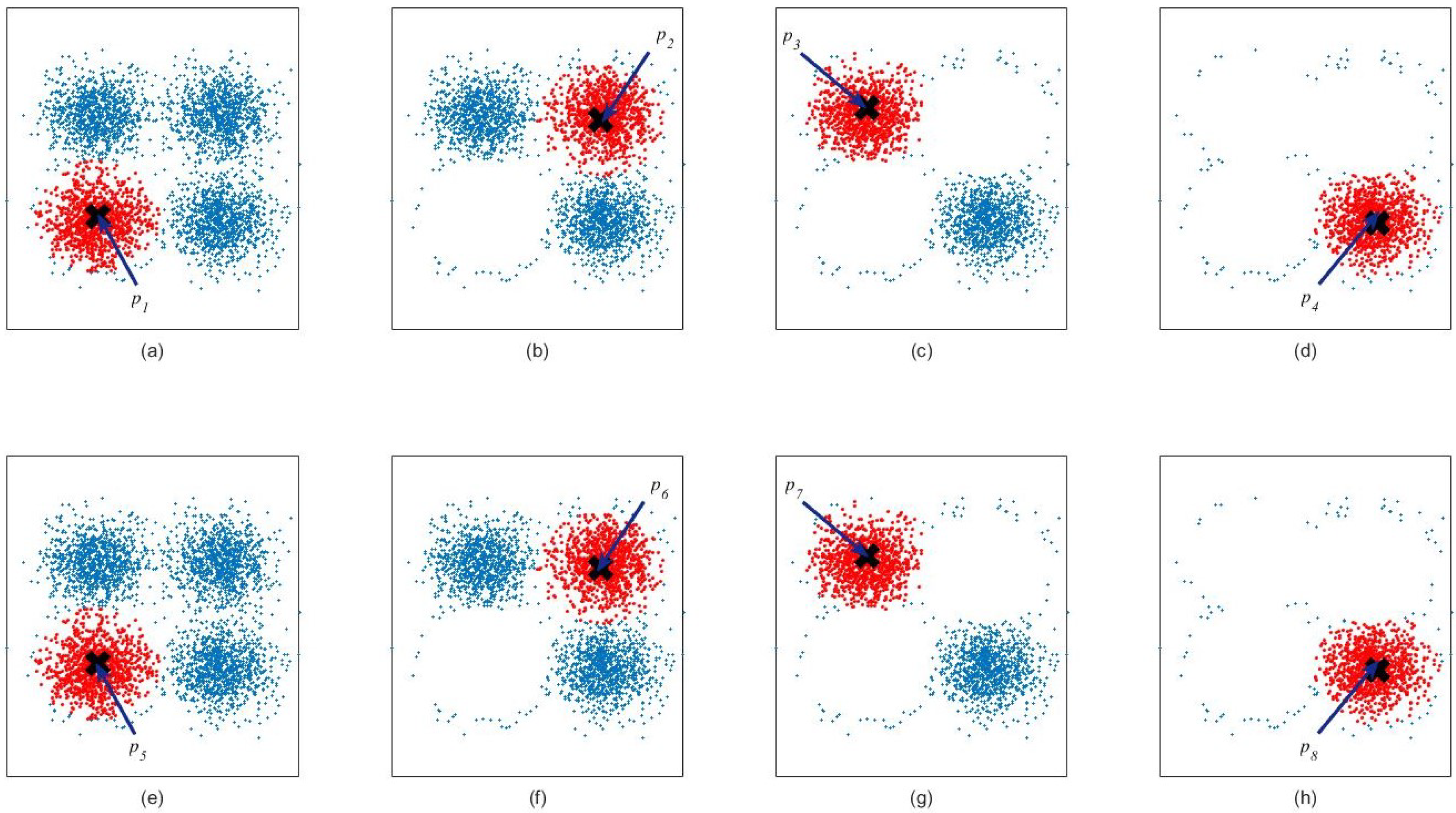
Pruning process of order selection under different neighborhood radius. The point in (a) represents the first cluster center, and , , in (b–d) represent the next cluster center, respectively. After is determined, the variance of the remaining points is larger than the threshold . The following four pictures (e–h) are the pruning results after the enlargement of the neighborhood radius. Under these two different radius conditions, due to , , , , it can be considered that the result is stable, relatively. Therefore, the order selection result of these data under this algorithm is 4. The neighborhood radius in the four graphs of the above part is , and in the other four graphs is . The abandoning threshold is , stable parameter M = 2.
Figure 4.
Pruning process of order selection under different neighborhood radius. The point in (a) represents the first cluster center, and , , in (b–d) represent the next cluster center, respectively. After is determined, the variance of the remaining points is larger than the threshold . The following four pictures (e–h) are the pruning results after the enlargement of the neighborhood radius. Under these two different radius conditions, due to , , , , it can be considered that the result is stable, relatively. Therefore, the order selection result of these data under this algorithm is 4. The neighborhood radius in the four graphs of the above part is , and in the other four graphs is . The abandoning threshold is , stable parameter M = 2.

Figure 5.
The order selection process, , .

Figure 6.
Illustration of order selection under the sparse matrix.

Figure 7.
Illustration of order selection under channel support matrix.

Figure 8.
Comparison of normalized mean square error under different algorithms.

Figure 9.
Lower and upper bounds of mutual information versus SNR.

Figure 10.
The relationship between the number of antennas and NMSE.

Figure 11.
The effect of on the performance.

Figure 12.
The effect of on the performance.


Table 1.
Parameters in simulation.
| Parameters | Configurations |
|---|---|
| 2048 | |
| N | 1024 |
| P | 200 |
| K | 16 |
| 0.3 | |
| 0.01 | |
| 50 | |
| 0.2 | |
| R | 50 |
| M | 3 |
© 2019 by the authors. Licensee MDPI, Basel, Switzerland. This article is an open access article distributed under the terms and conditions of the Creative Commons Attribution (CC BY) license (http://creativecommons.org/licenses/by/4.0/).
Share and Cite
MDPI and ACS Style
Chen, W.; Li, F.; Peng, Y. 3D-MIMO Channel Estimation under Non-Gaussian Noise with Unknown PDF. Electronics 2019, 8, 316. https://doi.org/10.3390/electronics8030316
AMA Style
Chen W, Li F, Peng Y. 3D-MIMO Channel Estimation under Non-Gaussian Noise with Unknown PDF. Electronics. 2019; 8(3):316. https://doi.org/10.3390/electronics8030316
Chicago/Turabian StyleChen, Wei, Feng Li, and Yiting Peng. 2019. "3D-MIMO Channel Estimation under Non-Gaussian Noise with Unknown PDF" Electronics 8, no. 3: 316. https://doi.org/10.3390/electronics8030316
Note that from the first issue of 2016, this journal uses article numbers instead of page numbers. See further details here.