LAP-SLAM: A Line-Assisted Point-Based Monocular VSLAM


1
School of Graduate, PLA Army Engineering University, Nanjing 210000, China
2
School of Field Engineering, PLA Army Engineering University, Nanjing 210000, China
*
Author to whom correspondence should be addressed.
Electronics 2019, 8(2), 243; https://doi.org/10.3390/electronics8020243
Submission received: 12 February 2019
/
Revised: 15 February 2019
/
Accepted: 17 February 2019
/
Published: 20 February 2019
(This article belongs to the Section Computer Science & Engineering)
Abstract
:While the performance of the state-of-the-art point-based VSLAM (vision simultaneous localization and mapping) systems in well textured sequences is impressive, their performance in poorly textured situations is not satisfactory enough. A sensible alternative or addition is to consider lines. In this paper, we propose a novel line-assisted point-based VSLAM algorithm (LAP-SLAM). Our algorithm uses lines without descriptor matching, and the lines are used to assist the computation conducted by points. To the best of our knowledge, this paper proposes a new way to include line information in VSLAM. The basic idea is to use the collinear relationship of points to optimize the current point-based VSLAM algorithm. In LAP-SLAM, we propose a practical algorithm to match lines and compute the collinear relationship of points, a line-assisted bundle adjustment approach and a modified perspective-n-point (PnP) approach. We built our system based on the architecture and pipeline of ORB-SLAM. We evaluate the proposed method on a diverse range of indoor sequences in the TUM dataset and compare with point-based and point-line-based methods. The results show that the accuracy of our algorithm is close to point-line-based VSLAM systems with a much faster speed.
1. Introduction
The past decade has witnessed a prosperous development in autonomous cars and unmanned vehicles. The simultaneous localization and mapping (SLAM) algorithms, which can estimate trajectories while reconstructing the unknown environment simultaneously, have proven effective and are the core technology of autonomous vehicles. Among the different sensor modalities of SLAM, visual SLAM (VSLAM) provides a solution with great potential because of its convenience and relatively low requirements for sensors.
There are mainly two kinds of mainstream techniques of VSLAM. Direct VSLAM approaches [1,2] directly use pixel intensities to match pixels across images and compute camera poses. These techniques can produce a dense [1] or semi-dense [2] reconstruction of the scene. While a dense reconstruction method reconstructs surfaces, a semi-dense method recovers the outer edges or surfaces with textures. However, the tracking is generally sensitive to illumination and does not have the function of loop closure. The feature-based VSLAM approaches [3,4] have relied on features. These techniques extract features from images, and then match the feature points from different images of different views. Compared with the direct method, the main strength of feature-based VSLAM is its accuracy and robustness.
The state-of-the-art visual odometry (VO) and visual SLAM (VSLAM) algorithms typically use point features, including the detection and matching of point features between frames. Then, they estimate the camera pose and location through least-squares minimization of the reprojection errors between the observed and projected points. The point features are simple to describe and manage, so they are widely studied and used in VSLAM. The state of the art VSLAM systems based on features, such as ORB-SLAM [3], can operate in indoors and outdoors environments in real-time, and be able to close loops and relocalize.
While the performance of state-of-the-art point-based VSLAM systems in well textured sequences is impressive, their performance in poorly textured situations, such as man-made scenarios, is not satisfactory enough. A sensible alternative or addition is considering lines because edges are also important features and are fairly abundant in images, especially in man-made environments. Man-made environments are characterized by regular structures that are rich in edges and linear shapes. Compared with points, the detection of lines is less sensitive to the noise associated with video capturing, and under a wide range of viewing angles, lines can be trivially stable [4].
Line features cannot be easily added to VSLAM, although there has been significant progress in line detection [5] and matching [6]. Line features are still difficult to represent [7]. Since lines occupy a much larger area than points and the line descriptors are much more complex, the computational burden of matching lines is much higher. Thus, the proposed solutions [8,9,10] are not much, barely reaching real-time specifications. Besides, regarding the expansion along its direction, line correspondences are generally weak to constrain. As a result, there can be a shift of the lines along their direction. The endpoints of line segments are hard to identify since it is common that only part of the lines can be observed because of occlusions or misdetections.
In this paper, we propose a novel line-assisted point-based VSLAM algorithm (LAP-SLAM) that is point-based with the assistance of lines, as shown in Figure 1. Unlike other common point-line-based VSLAM, which normally detect and match both lines and points in parallel, our algorithm matches lines without a descriptor, and uses the lines to assist the computation conducted by points. The accuracy of our system may not be as good as the common point-line-assisted VSLAM, but it can still improve the performance of point-based VSLAM, and the computation burden increased is much lower. In this way, the edge information of the scene can be used with a very low cost of computation resource. To the best of our knowledge, this paper explores a new way to make use of line information in VSLAM.
We match line segments through the matched points on them. In this way, line segments can be matched while ignoring the shift of the lines along their direction, and then the collinear relationship of the points and line segments across frames can be obtained. In this paper, we propose a practical algorithm to match lines and compute the collinear relationship of points. Based on the collinear relationship, a line-assisted bundle adjustment approach is proposed. In the perspective-n-point (PnP) problem of global relocalization, we also propose an approach, which considers the collinear relationship of points apart from points and lines information. We evaluate the proposed method in different scenes in TUM dataset [11], and compare it with the state-of-the-art point-based and point-line-based methods. The experimental results show that the model built by our algorithm can improve the performance of point-based VSLAM. Compared with other line-point-based VSLAM systems, the accuracy of our algorithm is close and the speed is much faster.
2. Related Work
Computing the trajectory of a camera from a continuous monocular image sequence while producing the 3D structure of the environment has been a hot topic and an important research field in computer vision and robotics in the past decade. This problem is known as SLAM. Most approaches rely on feature-based SLAM. The feature-based VSLAM approaches [3,12,13] have relied on features. These techniques extract features from images, and then match the feature points from different images of different views. The camera poses and coordinates of feature points are then jointly optimized by bundle adjustment (BA) [14]. The PTAM algorithm [12] represented a breakthrough in feature-based VSLAM. More recently, Mur-Artal et al. has proposed the ORB-SLAM [3] system, which provides a more robust camera tracking and mapping algorithm.
However, previous feature-based methods may lose track in environments with poor texture. In this case, dense and direct methods can solve this problem. Direct SLAM [15,16] optimizes the photometric error of sequential image registration over the space of possible pose changes between captured images. However, compared to feature-based methods, direct methods are more sensitive to several factors: Image noise, geometric distortion, large displacement, lighting change, etc. Therefore, feature-based methods are more viable as SLAM solutions for robust and accurate pose tracking.
Apart from points, line features are also widely studied in the field of VSLAM. Some representative early methods [17,18] use the Kalman filter. They use endpoint-pairs to parameterize 3D lines, then measure the residual of the projected lines on images. More recently, 3D visual sensors were considered in the systems of line-assisted VSLAM, such as stereo camera and RGB-D. A line-assisted RGB-D odometry system [19] was proposed in 2015. Besides, with the development of line detectors (e.g., LSD [5]) and descriptors (e.g., LBD [6]), more attention has been paid to stereo-based line VSLAM [8,10]. For line features, the distance between endpoints and lines is commonly used as the reprojection error. As to line features within monocular VSLAM, some representative works are as follows. PL-SLAM [10] has a pipeline similar to that of stereo methods. The study of [9] proposed a more robust variant for the endpoint-to-line distance. Line-assisted methods that are built based on direct VSLAM [20,21] have also been developed. To solve the problem that the 3D line input used in the least squares pose optimization is unreliable, a solution that extracts the most-informative sub-segment from each line has been proposed in [22]. The line residual of them is the least squares of the endpoint-to-line distance, the same as the other feature-based approaches.
Compared with point-based VSLAM, the additional parts of most line-assisted VSLAM are the detection, matching, and triangulation of lines. The high computation burden and the potential shift along the direction of lines are two main problems that are faced. The proposed LAP-SLAM matches lines through the matched points on them. In this way, the edge information of the scene can be used with a very low cost of computation resource, and the shift of the lines along their direction can be ignored. Our work is focused on building a practical algorithm to maintain and update the collinear relationship in real time, thus optimizing the bundle adjustment and PnP approach to consider the collinear relationship.
3. System Overview
The architecture of our approach is built based on that of the ORB-SLAM [3]. Compared with ORB-SLAM, our system integrates the information provided by lines and the collinear relationship (see Figure 2). ORB-SLAM is representative and one of the most complete and reliable featured-based vison SLAM systems. The ORB-SLAM system is based on ORB (oriented FAST and rotated BRIEF) features and uses three parallel threads, which are the tracking thread, local mapping thread, and loop closing thread. Now, we will briefly introduce these threads and emphasize the parts added by LAP-SLAM.
The tracking thread computes the poses of cameras and creates new keyframes. The constant velocity motion model is used to guess the current camera pose and initially match the current frame with the previous one. If the tracking is lost, the place recognition module will be used to relocalize the camera. In ORB-SLAM, this is typically achieved by the EPnP [23] algorithm—a non-iterative solution to the PnP problem. In LAP-SLAM, we add reprojection error between the detected lines and their correspondence points. The local mapping thread is mainly for local bundle adjustment. After the operations of keyframe insertion, map points culling, and new points creation, line segments in keyframes are detected by means of LSD. Then, we search the matched points on the line segments. For example, if two or more matched points are detected on a line segment of a keyframe, and the same points are detected on another line of another keyframe, these two line segments are matched and all the points on these line segments belong to one 3D line. The initial coordinate of the 3D line can be estimated, and then the location of the points belonging to this 3D line are adjusted on the 3D line. Afterwards, we run the line-assisted BA to optimize the poses of cameras, and the coordinates of the points and lines, with the cost function made up of the reprojection error of lines and points, and the distance between points and their corresponding lines. The loop closing thread processes the keyframe after the local mapping thread, and tries to check for loops, using only point features.
The work of this paper consists of three main parts: A practical algorithm to match lines and acquire the collinear relationship of points, a line-assisted bundle adjustment approach, and a PnP approach considering lines and the collinear relationship of points. The works are in the tracking thread and local mapping thread.
4. Matching of Line Segments and the Establishment of the Collinear Relationship
In LAP-SLAM, the collinear relationship is mainly built based on the matched points on different frames, and it is used in two functions: Line-assisted bundle adjustment and line-assisted global relocalization. The establishment of the collinear relationship is not operated in real-time, it runs when the system needs a collinear relationship. The first thing to do is to choose the related map points and keyframes in the map according to the collinear relationship needed. The choosing policy will be fully illustrated in Section 5.4. The creation and culling of keyframes and map points are unchanged in the LAP-SLAM compared with ORB-SLAM.
Specifically, the establishment of the relationship consists of the following several steps.
4.1. Detection of Line Segments
After acquiring the needed keyframes and map points, we use the LSD method [5] to detect the line segments of keyframes. LSD is a linear-time line segment detector that can achieve the accuracy of a subpixel. The LSD can work on any digital image and does not need to set parameters artificially. After detection, each line segment is numbered with an ID.
Then, the system generates an image of lines for each keyframe to assist the matching with map points. The image has the same size as the frames. The detected lines are drawn on the image, with their IDs stored in their colors. The other part of the image is black. To store the IDs of line segments, the IDs are converted to three numbers, and these three numbers are used as the BGR values of the colors of lines. The algorithm to convert the IDs into BGR values is shown as below (Algorithm 1):
| Algorithm 1: Algorithm to convert the ID into BGR values |
| Data: ID of line segment Result: RGB values R G B 1. B = floor((ID+1)/255/255); 2. if ((ID+1)%(255×255)==0) do 3. B=B-1; 4. G = floor(((ID+1-a×255×255))/255); 5. if (((ID+1-B×255×255))%255==0) do 6. G=G-1; 7. R = ID+1-B×255×255-G×255; |
| P. S. floor () is the rounding function. |
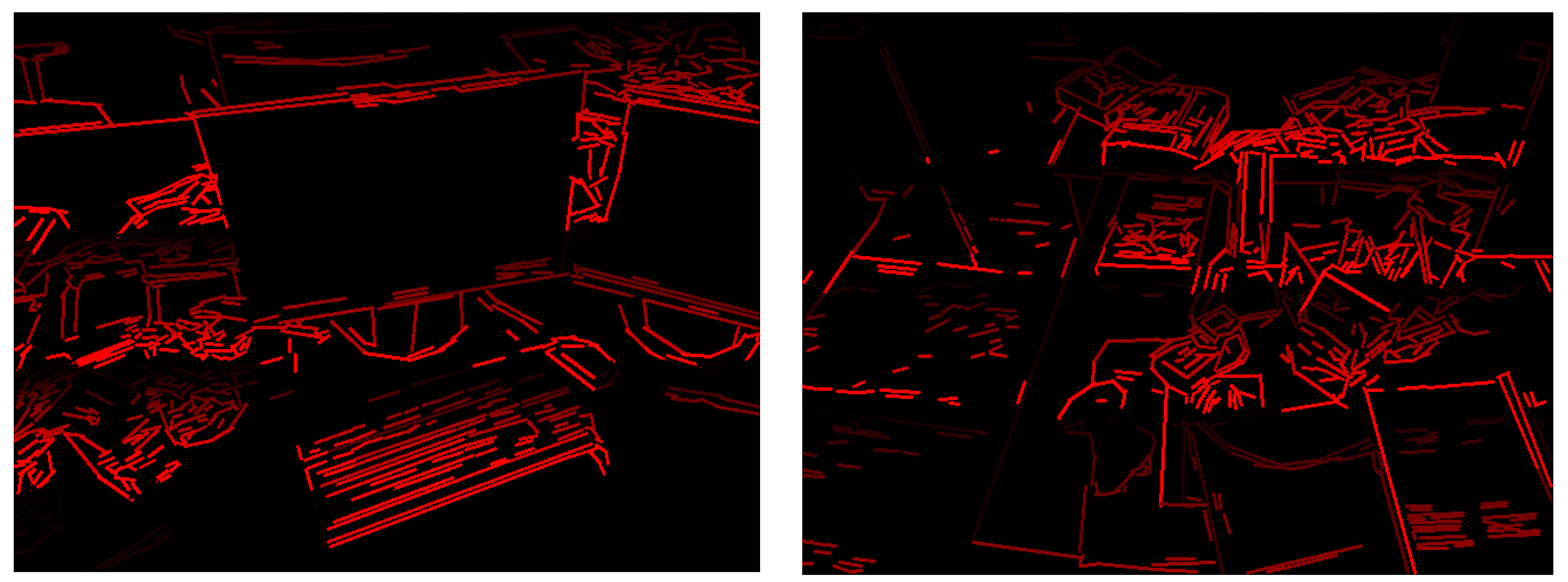
Two examples of the generated line images are shown in Figure 3.
4.2. Match Line Segments and Points
Each map point is projected on the line images. In every line image, the projection of the point will be discarded in the following circumstance: First, the projection is outside of the image bounds. Second, the angle between the current viewing ray, , and the map point mean viewing direction, , is more than , (). Third, the distance from the map point to the camera center is out of the scale invariance region of the map point.
After the projection, if the projected point on the line image passes the mentioned tests above, the system reads the BGR values of the projected point. If the values are all zero, it means the point is not projected on lines. If not, the point is projected on a line segment. The system then recovers the ID of the line segment from the BGR values of the point with the following equation:
The map points on every line segment are then recorded, as shown in the left of Figure 4.
4.3. Matching of Line Segments and the Establishment of the Collinear Relationship of Points
After the projection of all map points, all the correspondences of the lines and points are searched. If two or more matched points are detected on a line segment of a keyframe, and the same points are detected on another line of another keyframe, these two line segments are matched. If line segments are to be matched, the shared points of them should be more than two, in case the only shared point is at the intersection of two crossed lines. The system then generates a matrix to store the collinear relationship of line segments. Each row or column of the matrix represents a line segment. If two line segments are matched, the cross points of these line segments in the matrix are set as 1. If not, they are set as 0. After the search of all the correspondence, the collinear matrix of line segments has been built. Then, we search the matrix row by row and record all the line segments that belong to one 3D line. The method is briefly illustrated in Figure 4.
In this way, we can match line segments, even though there a shift along their direction exists, and some line segments cannot be directly matched with each other, as shown in Figure 5. After the matching, we can also get the collinear relationship of points, for all the points detected on the matched line segments are on the same 3D line.
5. Line-Assisted Bundle Adjustment
To integrate line and collinear relationship information with the current bundle adjustment, we need to define the line parameterization and error function. Apart from the basic point reprojection error, we define the line-based reprojection error and point collinear-constraint error. We next describe how this is integrated within bundle adjustment.
5.1. Line-Based Reprojection Error
To introduce lines to the ORB-SLAM, we need to properly define the reprojection error and parameterization of the line. are two random points on a 3D line, and they are used for the parameterization of the line. One 3D line has n correspondence line segments on different frames. represent the homogeneous coordinates of the projection of the points, P and Q, onto the frame plane. is the projected 3D line coefficient on the image plane of the i-th correspondence line segment. The normalized line coefficients are:
where K is the internal camera calibration matrix, and is the camera parameters. is the rotation parameters and is translation parameters, respectively.
are the endpoints of the i-th correspondence line segment. We define the line reprojection error, Eline, of a 3D line as the sum of the point-to-line distances, Epl, between all the endpoints of the detected line segments and their correspondence projected lines in their image planes (see Figure 6). That is:
with:
In the local mapping thread, before BA, we first use the line-based reprojection error to estimate the initial pose of the 3D line.
5.2. Point Collinear-Constraint Error
To add collinear constraint to map points on the same lines, we define point collinear-constraint error. One 3D line has m correspondence map points on it. are two random points on a 3D line. represents the homogeneous coordinates of them. The normalized line coefficient of the line is:
is the i-th correspondence map point. We then define the collinear-constraint error, Ecc, of a 3D line as the sum of point-to-line distances, Epl, between all the collinear map points and their correspondence 3D line (see Figure 7). That is:
with:
where is the 3D line coefficient.
5.3. Line-Assisted Bundle Adjustment
The camera pose and coordinates and points coordinates in the map are optimized through the bundle adjustment (BA) method. We build our BA based on the framework of the ORB-SLAM, but apart from point features, we also include the line features and collinear relationships. The specific cost function of our BA combines three types of geometric error, and it is defined as follows.
are the j-th map point. For the i-th keyframe, the coordinate of the projection of this point on the image plane is:
where is the pose of the i-th keyframe. is the observed coordinate of this point on the frame. We define the 3D error of points:
are two random points on the 3D correspondence line of the k-th detected line segments. The corresponding line projections onto the same keyframe are written as follow (expressed in homogeneous coordinates):
We estimate the coefficients of the projected line, , by using Equation (3). and are the observed endpoints of the k-th line segment. The error for the line is defined as follows:
The error (12) is actually an example of a point-to-line error (1).
are the l-th map point that is on a 3D line. are the two random points on the correspondence 3D line. The coefficients of the 3D line, , are estimated by Equation (6). The following collinear error of the map points on lines is defined as:
We obtain the comparable error representations for the points, lines, and the collinear relationship. Therefore, the unified cost function integrating each of the error terms is defined as:
where is the Huber robust cost function and , , , are the covariance matrices. They are associated with the scale at which the map points and line points were detected, respectively.
5.4. Line-Assisted BA in the LAP-SLAM
In the LAP-SLAM, the line-assisted BA is used in map initialization and local BA. Every time before line-assisted BA, the system will first establish the collinear relationship of these keyframes and map points involved, and then use the line-based reprojection error to estimate the initial pose of the 3D lines. These lines are also included and optimized in the lines-assisted BA together with the involved keyframes and map points, and these lines and their correspondences with map points are stored in maps after BA.
Map initialization computes the relative pose between two frames, triangulating an initial set of map points to initialize the system. As in the ORB-SLAM [3], our LAP-SLAM computes in parallel two geometrical models, a homography for a planar scene and a fundamental matrix for a non-planar scene. Then, one model is selected by a heuristic and used to recover the relative pose. Finally, in LAP-SLAM, we perform a full line-assisted BA to optimize the initial map. In the full line-assisted BA, we optimize the two keyframes and all points, except for the first keyframe, which remains fixed as the origin.
The local BA is in the local mapping thread. It runs after the system inserting keyframes. In LAP-SLAM, the current keyframe, all the keyframes are connected to it in the covisibility graph [24], and all the map points seen by those keyframes are optimized by the line-assisted local BA. All other keyframes that see those points, but are not connected to the current keyframe are included in the optimization, but remain fixed.
6. Global Relocalization
For any SLAM method, global relocalization is always an important part of it. When the tracker is lost, the system uses the approach to relocalize the camera. The PnP algorithm is a typical method of global relocalization, which tries to relocalize the current frame and estimate its pose based on its correspondences with 3D points in the map.
6.1. Line-Assisted EPnP
In ORB-SLAM, the used PnP method is EPnP [24], which only considers the point correspondences. In EPnPL [9], the EPnP is modified by adding line reprojection error. Through the algorithm mentioned before, once feature points on the current frame are matched with map points, we can get the line segments’ matches and the collinear relationship of the points. To make our approach appropriate for the consideration of lines and the collinear relationship for relocalization, we modify the EPnP by adding line reprojection error and collinear points’ reprojection error. To simultaneously consider points, lines correspondences, and collinear relationship, we modify the EPnP algorithm as follows.
In EPnP, is the projection of point X on the camera plane:
where are point-specific coefficients computed from the model and for j = 1,...,4 are the unknown control point coordinates on the frame. We define the vector of unknowns as .
Using Equations (3) and (4), we add the line-based reprojection error into EPnP, which is the sum of the point-to-line distances between all the detected line segment endpoints, , and their correspondence projected lines, , on the current frame as error. An expression for line reprojection error in case of EPnP is:
with:
where is the projected 3D line coefficient on the image plane of the i-th correspondence line segment, as defined in Equation (3).
Besides, to optimize the pose of the current camera, we also use the collinear relationship of points. However, unlike the in bundle adjustment, where we can use the sum of point-to-line distances between the 3D line and all its correspondence map points and to assist optimization, in global relocalization, the optimized parameter is only the pose of the camera, and the map points and 3D lines are fixed. Hence, we use the sum of the point-to-line distances of all collinear feature points, , and their projected correspondence lines, , on the current frame. An expression for collinear point-line reprojection error in the case of EPnP is:
with:
Finally, considering points, lines, and the collinear relationship of points, the function to be minimized by our modified EPnP is:
with:
where . is the matrix of parameters for the point correspondences. is the matrix of parameters for the line correspondences. is the matrix of parameters for the point-line correspondences. Equation (22) is finally minimized by the EPnP methodology.
6.2. Line-Assisted EPnP in LAP-SLAM
If the tracking is lost, the system converts the frame into a bag of words [25] and queries the recognition database for keyframe candidates for global relocalization. We compute the correspondences with ORB associated to map points. We then perform alternatively RANSAC iterations for each keyframe and try to find a camera pose using the line-assisted EPnP algorithm. The line-assisted EPnP uses the map points, their corresponding points on the current frame, and 3D lines in the map that are inserted after BA. Finally, the camera pose is optimized, and if supported with enough inliers, tracking thread continues.
7. Experimental Evaluation
We first evaluated the feasibility of our algorithm that matches detected line segments through matched points. Then, we compared the accuracy of our LAP-SLAM system with some state-of-the-art VSLAM systems using the TUM benchmark and real data. Besides, we also compared the computation time of our LAP-SLAM with ORB-SLAM and PL-SLAM. All experiments were conducted on a laptop with an Intel i7-7700HQ processor (4 cores at 2.8 GHz) and 8 Gb memory. Due to the randomness throughout the process, all experiments were operated three times and recorded as an average.
7.1. Match of Line Segments
To evaluate the feasibility of our algorithm that matches detected line segments through matched points, we compared our algorithm and the LBD method that is widely used. In total, 30 picture pairs from 5 sequences of TUM and 10 picture pairs from our hand-held camera were tested by both our algorithm and the LBD method. The average number of matched line segments and time spent are shown in Table 1.
From the results, it can be seen that compared with the LBD method, our algorithm matches fewer line segments, because our algorithm matches line segments through matched points. The line segments can only be matched if there are two or more matched points on them. The LBD method computes and matches the descriptor of every line segment, so it can match more lines.
The time used by our method is much shorter and is positively correlated with the number of detected line segments. The computation and matching of the line segment descriptor is more complex than points, and will cost more computation time. Because our algorithm does not compute and match the descriptors of line segments, its speed is much faster.
Besides, as shown in Figure 8, compared with LBD, the main and representative line segments can be matched by our algorithm. These matched lines can cover most of the matched points in the image, and they can be used to assist the points by building a collinear relationship. In conclusion, our algorithm is feasible, and can achieve the expected functionality of matching lines and establishing a collinear relationship with satisfactory speed.
We then evaluated the application of our algorithm in LAP-SLAM. Table 2 shows the numbers of lines and points in the maps created by LAP-SLAM in different sequences. It can be seen that their numbers are roughly positively related. The more points created in the map, the more lines can be matched and put into the map.
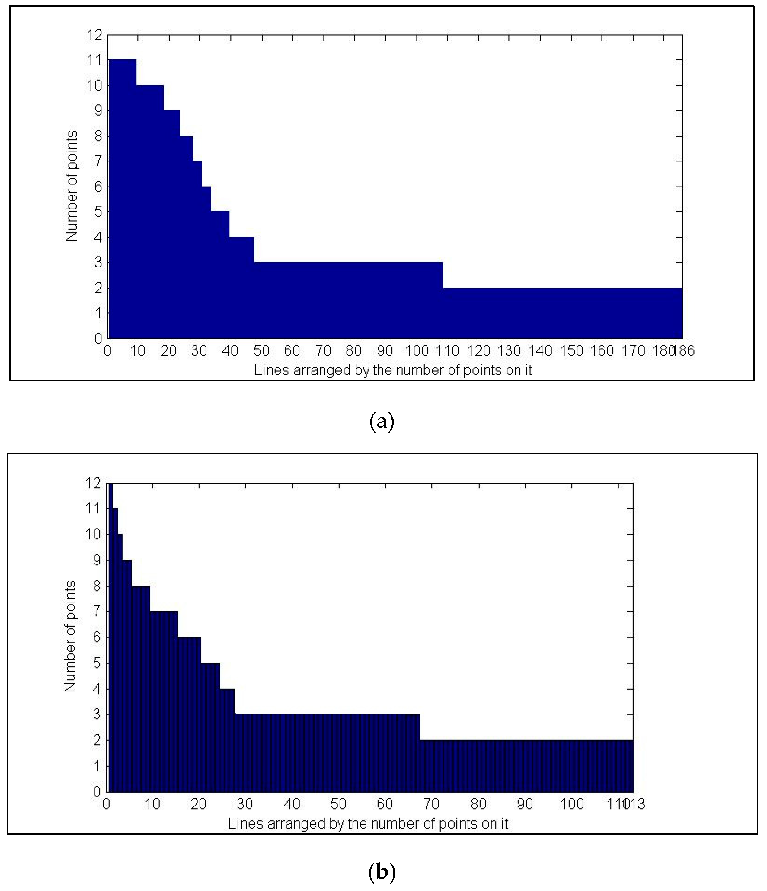
Then, we analyzed the collinear relationship built by our system by recording the number of points on each line. Figure 9 shows two histograms of lines according to the number of points on them. From the histograms, we can see that there are some respective lines that are associated with more points than others. Most lines are short and are associated with less than five points.
7.2. Relocalization
To evaluate the relocalization ability of LAP-SLAM, we performed an experiment of relocalization in two sequences of the TUM dataset. The same experiments were performed on LAP-SLAM and ORB-SLAM for comparison. In the experiments, maps were built from the first 30 s of the sequences. We then performed global relocalization with every successive frame and recorded the accuracy of the recovered poses. The recall rate and the error with respect to the ground truth are shown in Table 3. We can see from the results that the frames relocalized by the LAP-SLAM and ORB-SLAM are nearly the same, because they use the same method to check for loops. However, the accuracy of our LAP-SLAM is higher.
7.3. Localization Accuracy
To test the localization accuracy of LAP-SLAM, we compared our method with two current state-of-the-art point-based VSLAM methods, ORB-SLAM and LSD-SLAM, and a point-line-based VSLAM, PL-SLAM. The absolute trajectory error (ATE) was used for comparison. Before computing the ATE error, all trajectories were aligned with the ground truth with 7 DoF. The ground truth data was provided by the benchmark. The results are summarized in Table 4.
Note that our LAP-SLAM consistently improves the trajectory accuracy of ORB-SLAM in all sequences. LSD-SLAM lost track in 3 out of 11 sequences, respectively. Compared with point-based SLAM, our method adds the information of the lines and collinear relationship in the optimization, which can provide the optimization with a more accurate cost function.
Indeed, the accuracy of LAP-SLAM is lower than that of PL-SLAM, because the point-line based SLAM, like PL-SLAM, has more matched lines and thus means more input information. However, the gap between their accuracy is not obvious. In some sequences, the accuracy of LAP-SLAM is very close to and can nearly match the accuracy of PL-SLAM. These sequences where LAP-SLAM performs well share the characteristics that there are main and respective lines in the scene and multiple feature points can be detected on these lines. The collinear relationship of points can help a lot in this circumstance.
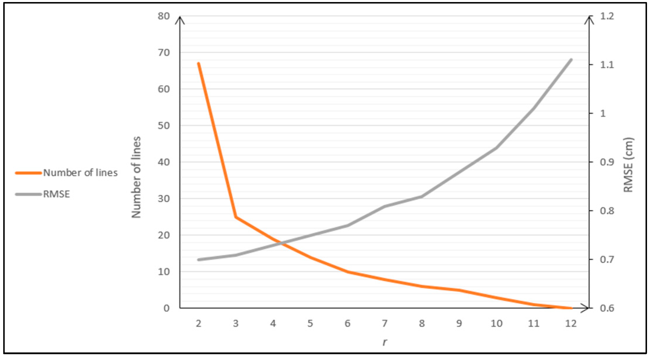
To further evaluate the effect of our line-assisted method, we then performed an experiment on an example sequence, fr2_desk, of TUM. In this experiment, we defined a restriction parameter, r, which means the lines with fewer than r corresponding points were abandoned. The change of accuracy of LAP-SLAM and the number of lines in the final map with r is shown in Figure 10.
From the figure, it can be seen that the lines with few corresponding points are a lot, but they have relatively little influence on the RMSE. In general, the RMSE rises and the lines decrease as r increases. The lines that have more than eight points on them play a major role in improving the accuracy.
7.4. Computation Time
While introducing line information to the VSLAM improves accuracy, it also increases the computational burden of the system. Table 5 summarizes the time used in each subtask in the threads of “Tracking” and “Local Mapping”, for LAP-SLAM, PL-SLAM, and ORB-SLAM. The time recorded is the average computation time of five different sequences of the TUM sequences.
Compared with ORB-SLAM, the time consumed by LAP-SLAM is longer, but much shorter than that of PL-SLAM. The tracking thread of LAP-SLAM and ORB-SLAM is the same, because LAP-SLAM only extracts and matches line features in keyframes in local mapping. The subtask with the largest cost of time is the map feature creation and the local BA. Note that the feature creation of LAP-SLAM includes the operation of the extract and match line features in keyframes, but LAP-SLAM are still faster than PL-SLAM in these subtasks for less features. In all the sequences, the final frame rate of the LAP-SLAM can operate in real time on a normal computer.
8. Conclusions
In this paper, we propose LAP-SLAM, an algorithm that is based on points, but also uses the information of lines as assistance. In LAP-SLAM, the lines are not used as in other common point-line-based VSLAM, which normally detect and match both lines and points in parallel. We matched lines without a descriptor through the matched points on them. Since the computation and matching of the line descriptor is very time consuming, the matching speed of our method is much faster. We proposed a practical algorithm to match lines and compute the collinear relationship of points. In this way, although the number of matched lines are fewer, the main and representative lines can still be matched. The edge information of the scene can be used with a very low cost of computation resources. These matched line segments in LAP-SLAM are used to establish the collinear relationship of points. The collinear relationship is included in LAP-SLAM, and it is the main contribution of our paper. The current point-based VSLAM algorithm was optimized by adding the collinear relationship. Specifically, in this work, a line-assisted bundle adjustment approach and a PnP approach considering lines and the collinear relationship of points were proposed. To the best of our knowledge, this paper proposes a new way to include line information in VSLAM. We built upon the architecture of state-of-the-art ORB-SLAM and modified its original pipeline without significantly compromising its efficiency. We evaluated the proposed method on a diverse range of indoor scenes in the TUM dataset and compared it with state-of-the-art point-based and point-line-based VSLAM systems. The results show that our method can improve the accuracy of point-based VSLAM, and even close to point-line-based VSLAM. Compared with point-line based VSLAM, although the accuracy of LAP-SLAM is a little lower, the time consumed is much shorter. In other words, our method can improve the VSLAM system in a relatively more efficient way.
In future work, we plan to further exploit line features and incorporate other geometric primitives, like planes, which can be built from lines in a similar manner as we have built lines from point features.
Author Contributions
F.Z. and T.R. conceived and designed the experiments; F.Z. performed the experiments; F.Z. and C.Y. analyzed the data; J.S. contributed analysis tools; F.Z. wrote the paper.
Funding
This research received no external funding.
Conflicts of Interest
The authors declare no conflict of interest.
References
- Newcombe, R.A.; Lovegrove, S.J.; Davison, A.J. DTAM: Dense tracking and mapping in real-time. In Proceedings of the IEEE International Conference on Computer Vision (ICCV), Barcelona, Spain, 6–13 November 2011; pp. 2320–2327. [Google Scholar]
- Engel, J.; Schöps, T.; Cremers, D. LSD-SLAM: Large-scale direct monocular SLAM. In Proceedings of the European Conference on Computer Vision (ECCV), Zurich, Switzerland, 6–12 September 2014; pp. 834–849. [Google Scholar]
- Mur-Artal, R.; Montiel, J.M.M.; Tardós, J.D. ORB-SLAM: A Versatile and Accurate Monocular SLAM System. IEEE Trans. Robot. 2015, 31, 1147–1163. [Google Scholar] [CrossRef]
- Gee, A.P.; Mayol-Cuevas, W. Real-time model-based slam using line segments. In International Symposium on Visual Computing; Springer: Berlin/Heidelberg, Germany, 2006; pp. 354–363. [Google Scholar]
- Von Gioi, R.G.; Jakubowicz, J.; Morel, J.-M.; Randall, G. LSD: A Fast Line Segment Detector with a False Detection Control. IEEE Trans. Softw. Eng. 2010, 32, 722–732. [Google Scholar] [CrossRef] [PubMed]
- Zhang, L.; Koch, R. Line matching using appearance similarities and geometric constraints. In Proceedings of the Pattern Recognition: Joint 34th DAGM and 36th OAGM Symposium, Graz, Austria, 28–31 August 2012; pp. 236–245. [Google Scholar]
- Bartoli, A.; Sturm, P. Structure-from-motion using lines: Representation, triangulation, and bundle adjustment. Comput. Visi. Image Understand. 2005, 100, 416–441. [Google Scholar] [CrossRef]
- Koletschka, T.; Puig, L.; Daniilidis, K. MEVO: Multienvironment stereo visual odometry. In Proceedings of the 2014 IEEE/RSJ International Conference on Intelligent Robots and Systems, Chicago, IL, USA, 14–18 September 2014; pp. 4981–4988. [Google Scholar]
- Vakhitov, A.; Funke, J.; Moreno-Noguer, F. Accurate and linear time pose estimation from points and lines. In Proceedings of the European Conference on Computer Vision, Amsterdam, The Netherlands, 11–14 October 2016; Springer: Berlin/Heidelberg, Germany, 2016; pp. 583–599. [Google Scholar]
- Pumarola, A.; Vakhitov, A.; Agudo, A.; Sanfeliu, A.; Moreno-Noguer, F. Pl-slam: Real-time monocular visual slam with points and lines. In Proceedings of the IEEE International Conference on Robotics and Automation (ICRA), Singapore, 29 May–3 June 2017; pp. 4503–4508. [Google Scholar]
- Huitl, R.; Schroth, G.; Hilsenbeck, S.; Schweiger, F.; Steinbach, E. TUM indoor: An extensive image and point cloud dataset for visual indoor localization and mapping. In Proceedings of the IEEE International Conference on Image Processing, Melbourne, Australia, 15–18 September 2013; pp. 1773–1776. [Google Scholar]
- Klein, G.; Murray, D. Parallel tracking and mapping for small AR workspaces. In Proceedings of the IEEE and ACM International Symposium on Mixed and Augmented Reality (ISMAR), Nara, Japan, 13–16 November 2007; pp. 225–234. [Google Scholar]
- Davison, A.J.; Reid, I.D.; Molton, N.D.; Stasse, O. MonoSLAM: Real-time single camera SLAM. IEEE Trans. Pattern Anal. Mach. Intell. 2007, 29, 1052–1067. [Google Scholar] [CrossRef] [PubMed]
- Triggs, B.; McLauchlan, P.F.; Hartley, R.I.; Fitzgibbon, A.W. Bundle adjustment a modern synthesis. In Vision Algorithms: Theory and Practice; Springer: Berlin/Heidelberg, Germany, 2000; pp. 298–372. [Google Scholar]
- Forster, C.; Zhang, Z.; Gassner, M.; Werlberger, M.; Scaramuzza, D. Svo: Semidirect visual odometry for monocular and multicamera systems. IEEE Trans. Robot. 2016, 33, 249–265. [Google Scholar] [CrossRef]
- Engel, J.; Koltun, V.; Cremers, D. Direct sparse odometry. IEEE Trans. Pattern Anal. Mach. Intell. 2018, 40, 611–625. [Google Scholar] [CrossRef] [PubMed]
- Smith, P.; Reid, I.D.; Davison, A.J. Real-Time Monocular SLAM with Straight Lines. In Proceedings of the British Machine Conference, Edinburgh, UK, 4–7 September 2006; BMVA Press: Edinburgh, UK; Chantler, M., Fisher, B., Trucco, M., Eds.; BMVA Press: Edinburgh, UK, 2006; pp. 3.1–3.10. [Google Scholar]
- Gomez-Ojeda, R.; Moreno, F.; Scaramuzza, D.; Gonzalez-Jimenez, J. Pl-slam: A stereo slam system through the combination of points and line segments. arXiv, 2017; arXiv:1705.09479. [Google Scholar]
- Lu, Y.; Song, D. Robust rgb-d odometry using point and line features. In Proceedings of the IEEE International Conference on Computer Vision, Santiago, Chile, 7–13 December 2015; pp. 3934–3942. [Google Scholar]
- Gomez-Ojeda, R.; Briales, J.; Gonzalez-Jimenez, J. Pl-svo: Semidirect monocular visual odometry by combining points and line segments. In Proceedings of the IEEE/RSJ International Conference on Intelligent Robots and Systems (IROS), Daejeon, Korea, 9–14 October 2016; pp. 4211–4216. [Google Scholar]
- Yang, S.; Scherer, S. Direct monocular odometry using points and lines. In Proceedings of the IEEE International Conference on Robotics and Automation (ICRA), Singapore, 29 May–3 June 2017; pp. 3871–3877. [Google Scholar]
- Zhao, Y.; Vela, P.A. Good Line Cutting: Towards Accurate Pose Tracking of Line-assisted VO/VSLAM. In Proceedings of the Computer Vision, ECCV, Munich, Germany, 8–14 September 2018. [Google Scholar]
- Lepetit, V.; Moreno-Noguer, F.; Fua, P. Epnp: An accurate o(n) solution to the pnp problem. Int. J. Comput. Vis. 2009, 81, 155–166. [Google Scholar] [CrossRef]
- Mei, C.; Sibley, G.; Newman, P. Closing loops without places. In Proceedings of the 2010 IEEE/RSJ International Conference on Intelligent Robots and Systems, Taipei, Taiwan, 18–22 October 2010. [Google Scholar]
- GálvezLópez, D.; Tardós, J.D. Bags of binary words for fast place recognition in image sequences. IEEE Trans. Robot. 2012, 28, 1188–1197. [Google Scholar] [CrossRef]
Figure 1.
A toy case illustrating the proposed LAP-SLAM approach. (a) The initial coordinates of the points and poses of cameras are calculated through the geometric method, as normal point-based SLAM. (b) If two or more points are matched, such as A and B, and they are on the same detected line segments in different frames, these line segments are matched. Besides, we get the collinear relationship of A, B, and C. These line segments on different frames are parts of the projection of a 3D line, and the initial coordinate of the 3D line can be estimated from these line segments. (c) Then, we run the line-assisted bundle adjustment (BA), to optimize the poses of cameras, and coordinates of points and lines, considering the collinear relationship (the optimized parameters are framed by red dashed lines).

Figure 2.
LAP-SLAM pipeline is an extension of that of ORB-SLAM [3]. The system consists of three main threads: Tracking thread, local mapping thread, and loop closing thread. The tracking thread estimates the position and pose of the camera, and makes the decision of adding new keyframes. Then, the local mapping thread adds the new keyframe into the map and optimizes the information in the local map with BA. The additional line-assisted operations are mainly added in this thread. The loop closing thread is in charge of checking for loops and correcting the accumulated error through loop closure. The two blocks surrounded by red dashed rectangles are the main novel work of this paper.

Figure 3.
Two examples of the generated line images. The R values calculated by our algorithm is the largest and changes fastest, so the red is the most obvious color in the images.
Figure 3.
Two examples of the generated line images. The R values calculated by our algorithm is the largest and changes fastest, so the red is the most obvious color in the images.

Figure 4.
A toy case illustrating the proposed method of matching line segments. On the left is the correspondence of line segments and map points, where A, B, …, E represents line segments and colorful balls are points. The collinear matrix in the middle is built from the search and match from the correspondence. From the matrix, we can get the collinear relationship of line segments.

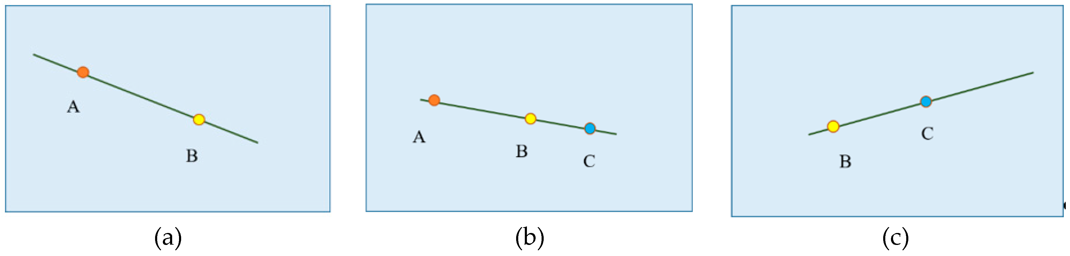
Figure 5.
An example of the establishment of a collinear relationship. From the correspondence between lines and points, we can match the line segments in frame 1 (a) and frame 2 (b), and frame 3 (c). In this way, we know all three line segments are parts of the projection of one 3D line, ignoring the shift of endpoints, and all the three points are on this 3D line.

Figure 6.
Line reprojection error. The green dashed line, , represents the projected 3D line on the image plane. are the endpoints of the i-th correspondence line segment. Red lines, and , are the line reprojection error between a projected 3D line (green dashed) and the corresponding detected 2D line (green solid). The line-based reprojection error of a 3D line is the sum of the line reprojection error of all the correspondence line segments.

Figure 7.
Point collinear-constraint error. The green line, , represents the 3D line. Red lines, , , and , are point-to-line distances between the 3D line and its corresponding map points. The point collinear-constraint error of a 3D line is the sum of point-to-line distances between the 3D line and all its corresponding collinear map points.

Figure 8.
Examples of matches: (a) TUM fr1_xyz; (b) hand-held camera. Line segments are detected by LSD (left) and matched by our algorithm (middle) and LBD (right) in an example pair of pictures from TUM fr1_xyz. The matched line segments are numbered and drawn on one picture of the pair. In the middle picture of our algorithm, the ORB feature points are marked by colorful circles.

Figure 9.
Histogram of the numbers of points of all lines. (a) TUM fr1_xyz; (b) TUM fr2_desk.

Figure 10.
Change of RMSE of LAP-SLAM and the number of lines with r.


Table 1.
Comparison of our algorithm and the LBD method.
| Sequence | Average Numbers of Matched Line Segments | Average Time Consumed (s) | ||
|---|---|---|---|---|
| Ours | LBD | Ours | LBD | |
| fr1_xyz | 55 | 163 | 0.29 | 0.72 |
| fr1_floor | 51 | 139 | 0.30 | 0.81 |
| fr2_xyz | 62 | 170 | 0.33 | 1.10 |
| fr2_desk | 45 | 154 | 0.15 | 0.98 |
| fr3_long_office | 57 | 256 | 0.28 | 0.76 |
| hand-held camera | 50 | 198 | 0.27 | 0.93 |
Table 2.
The numbers of lines and points in maps created by LAP-SLAM.
| Sequence | Line | Point |
|---|---|---|
| fr1_xyz | 186 | 2403 |
| fr1_floor | 150 | 2034 |
| fr2_xyz | 235 | 2605 |
| fr2_desk | 113 | 1971 |
| fr3_long_office | 151 | 2258 |
| fr3_str_tex_near | 166 | 2311 |
Table 3.
Results of the relocalization experiments.
| TUM Sequence | fr1_xyz | fr3_walk_xyz | ||||
|---|---|---|---|---|---|---|
| Initial Map | System | LAP-SLAM | ORB-SLAM [3] | LAP-SLAM | ORB-SLAM [3] | |
| KFs | 24 | 24 | 32 | 31 | ||
| RMSE (cm) | 0.18 | 0.19 | 0.36 | 0.38 | ||
| Relocalization | Recall (%) | 77.1 | 78.3 | 78.2 | 77.9 | |
| RMSE (cm) | 0.35 | 0.38 | 1.21 | 1.32 | ||
| Max Error (cm) | 1.52 | 1.67 | 4.68 | 4.95 | ||
Table 4.
Localization accuracy in the TUM RGB-D benchmark.
| TUM Sequence | Absolute Keyframe Trajectory RMSE (cm) | |||
|---|---|---|---|---|
| LAP-SLAM | ORB-SLAM | PL-SLAM [10] | LSD-SLAM | |
| fr1_xyz | 1.34 | 1.34 | 1.30 | 10.15 |
| fr1_floor | 7.85 | 8.12 | 7.82 | 42.66 |
| fr2_xyz | 0.46 | 0.47 | 0.43 | 3.65 |
| fr2_desk | 0.70 | 1.11 | 0.64 | 5.11 |
| fr2_desk_person | 2.75 | 3.24 | 2.15 | 35.63 |
| fr2_360_kidnap | 4.12 | 4.46 | 4.09 | — |
| fr3_long_office | 2.45 | 3.75 | 2.17 | 31.92 |
| fr3_str_tex_near | 1.31 | 1.62 | 1.25 | — |
| fr3_sit_xyz | 0.27 | 0.81 | 0.16 | 5.36 |
| fr3_walk_xyz | 1.54 | 1.56 | 1.54 | 12.47 |
| fr3_walk_halfsph | 1.76 | 1.97 | 1.71 | — |
Table 5.
Average execution time consumed in tracking and local mapping.
| Thread | Operation | Average Execution Time (ms) | ||
|---|---|---|---|---|
| LAP-SLAM | ORB-SLAM | PL-SLAM [10] | ||
| Tracking | Feature Extraction | 15.91 | 15.84 | 44.36 |
| Initial Estimation | 11.18 | 11.29 | 11.58 | |
| Track Local Map | 5.22 | 5.14 | 18.75 | |
| Total | 32.31 | 32.27 | 74.69 | |
| Local Mapping | Keyframe Insertion | 14.91 | 14.79 | 25.62 |
| Feature Culling | 1.69 | 1.72 | 1.77 | |
| Feature Creation | 83.68 | 12.59 | 119.42 | |
| Local BA | 303.55 | 189.61 | 349.23 | |
| Keyframe Culling | 4.87 | 4.23 | 17.78 | |
| Total | 358.70 | 222.94 | 513.82 | |
© 2019 by the authors. Licensee MDPI, Basel, Switzerland. This article is an open access article distributed under the terms and conditions of the Creative Commons Attribution (CC BY) license (http://creativecommons.org/licenses/by/4.0/).
Share and Cite
MDPI and ACS Style
Zhang, F.; Rui, T.; Yang, C.; Shi, J. LAP-SLAM: A Line-Assisted Point-Based Monocular VSLAM. Electronics 2019, 8, 243. https://doi.org/10.3390/electronics8020243
AMA Style
Zhang F, Rui T, Yang C, Shi J. LAP-SLAM: A Line-Assisted Point-Based Monocular VSLAM. Electronics. 2019; 8(2):243. https://doi.org/10.3390/electronics8020243
Chicago/Turabian StyleZhang, Fukai, Ting Rui, Chengsong Yang, and Jianjun Shi. 2019. "LAP-SLAM: A Line-Assisted Point-Based Monocular VSLAM" Electronics 8, no. 2: 243. https://doi.org/10.3390/electronics8020243
Note that from the first issue of 2016, this journal uses article numbers instead of page numbers. See further details here.