Constant Envelope Modulation Techniques for Limited Power Millimeter Wave Links


Faculty of Engineering, Ariel University, Ariel 40700, Israel
*
Author to whom correspondence should be addressed.
Electronics 2019, 8(12), 1521; https://doi.org/10.3390/electronics8121521
Submission received: 18 November 2019
/
Revised: 30 November 2019
/
Accepted: 3 December 2019
/
Published: 11 December 2019
(This article belongs to the Collection Millimeter and Terahertz Wireless Communications)
Abstract
:The demand for increased capacity and link availability for mobile communications requires the utilization of higher frequencies, such as millimeter waves at extremely high frequencies (EHFs) above 30 GHz. In this regime of frequencies, the waves are subjected to high atmospheric attenuation and dispersion effects that lead to a degradation in communication reliability. The fact that solid-state millimeter and sub-millimeter wave sources are producing low power calls for effective signaling utilizing waveforms with a low peak to average power ratio (PAPR), such as constant envelope (CE) modulation. The CE techniques present a PAPR of 0 dB resulting in peak power transmission with high energy efficiency. The study of the performances of constant envelope orthogonal modulation techniques in the presence of co-channel interference is presented. The performance is evaluated in terms of the average symbol error rate (SER) using analytical results and simulations. The theory is carried out for the CE-M-ary time orthogonal (CE-MTO) and CE-orthogonal frequency division multiplexing (CE-OFDM), demonstrating comparable performances while leading to a simpler implementation than that of the CE-OFDM.
1. Introduction
Wireless communications require more bandwidth because of the necessity of the capacity increasing, the availability, and the reliability. As a result, new bands need to be searched for in the electromagnetic spectrum, reaching millimeter and sub-millimeter wavelengths. Recent technological developments have made extremely high frequencies (EHF) a candidate for wireless applications, such as for the fifth generation (5G) of cellular communications (for which bands in the 24.25–29.5 GHz and 37–43.5 GHz are already allocated [1]), satellite communications [2,3], high resolution radars [4,5], and remote sensing [6,7]. The realization of wireless communications in the millimeter wavelength systems is becoming commercial, compact, and less expensive [8,9].
However, the fact that the atmospheric medium is not entirely transparent to millimeter waves (MMWs) requires careful considerations regarding the frequency selective absorption and dispersion effects emerging in this band [10]. Moreover, low power transmissions and reduced receiver sensitivities lead to further degradation in the link performances [11]. These phenomena also apply to radars and remote sensing systems operating in the millimeter and Terahertz frequencies [12].
While the bands in the ultra-high frequency (UHF) spectrum are fully used, millimeter waves (the EHF spectrum) are relatively free of users, and broad bands of frequencies can be allocated for wireless communication applications. With the demand for more spectrums for the mobile communication infrastructure, additional bands within the millimeter waves regime are allocated for the future 5G of the cellular networks [13]. The extension of the spectrums enables ultra-reliable low-latency communication (URLLC) broadband services, with faster access and an increased capacity. The short wavelength of the millimeter waves enables the utilization of small equipment and antennas. The MMW cell will be a few hundredths of a meter, having multiple antennas communicating in a massive multiple-input multiple-output (MIMO) arrangement [14,15]. Beamforming techniques will allow for the operation of multiple antennas to direct the transmission to the operators [16,17,18].
The power produced by solid-state devices is limited to several tens of milli-watts in MMWs. This limitation calls for effective signaling utilizing constant envelope (CE) waveforms with a low peak to average power ratio (PAPR). The utilization of constant envelope techniques enables a non-linear class of operation, resulting in a better efficiency of energy consumption. This is particularly important for battery-powered mobile appliances because of their limited power resources [19,20,21].
Constant envelope (CE) orthogonal signaling is proposed as an efficient modulation technique for wireless communication systems [22,23]. The peak to average power ratio (PAPR) in a CE waveform is 0 dB. The popular orthogonal frequency division multiplexing (OFDM) signaling, which is commonly used in communications, presents envelope fluctuations, resulting in a high PAPR [24].
Several CE techniques have been suggested. In the literature [25,26], the information-bearing message signal is transformed into a constant envelope waveform by the utilization of the phase modulation. In the CE-OFDM discussed in the literature [25], the OFDM waveform is used to phase modulate the carrier, while in our proposed CE-M-ary time orthogonal (CE-MTO) technique described in [26], orthogonal waveforms in the time domain were used. In our previous work [26], we showed that the implementation of the CE-MTO technique is expected to be simpler than that of the CE-OFDM, and that the symbol error rate (SER) performances in the presence of additive white gaussian noise (AWGN) and fading channels are comparable for both techniques.
Interference is a significant challenge of wireless communications that has a detrimental effect on the overall link performances. Although it cannot be completely mitigated, the interference effect can be reduced to a certain extent. Several types of interferences exist [27], one of which is co-channel interference (CCI) [28]. It occurs when the interfering signal overlaps with the desired signal in the frequency domain. In order to mitigate the CCI, many methods have been proposed [29,30,31,32]. Channel coding is a traditional and effective way to reduce the CCI, and also provides some robustness [33].
In this paper, we examine the symbol error rate (SER) in the presence of CCI and AWGN, for both CE-OFDM and CE-MTO techniques. An analytical expression is derived, from which one can estimate the degradation caused by the CCI in an MMW channel employing constant envelope signaling.
In Section 2, we review the link budgets for the required signal and the interfering one, both operating in the millimeter wave regime. Section 3 presents an analytic study of the detection for a constant envelope modulated signal in the presence of co-channel interference. In Section 4, additive white Gaussian noise is added to the analysis for calculating the symbol error rate. The simulation results are given in Section 5 for different CCI scenarios. A comparison is made with the results obtained from the analytical calculations. Section 6 summarizes and concludes the paper.
2. Communication Links in Millimeter Waves
When the electromagnetic radiation in the millimeter wavelengths and terahertz frequencies regime propagates through the atmosphere, it experiences selective molecular absorptions [34,35,36,37,38,39,40]. Several empirical and analytical models have been suggested for estimating the millimeter and sub-millimeter wave transmission of the atmospheric medium. The transmission characteristics of the atmosphere at the EHF band were calculated using the millimeter propagation model (MPM), developed by Liebe [41,42,43,44]. The inhomogeneous atmospheric transmission affects the amplitude and phase of the signals transmitted in the millimeter and sub-millimeter wavelengths [45].
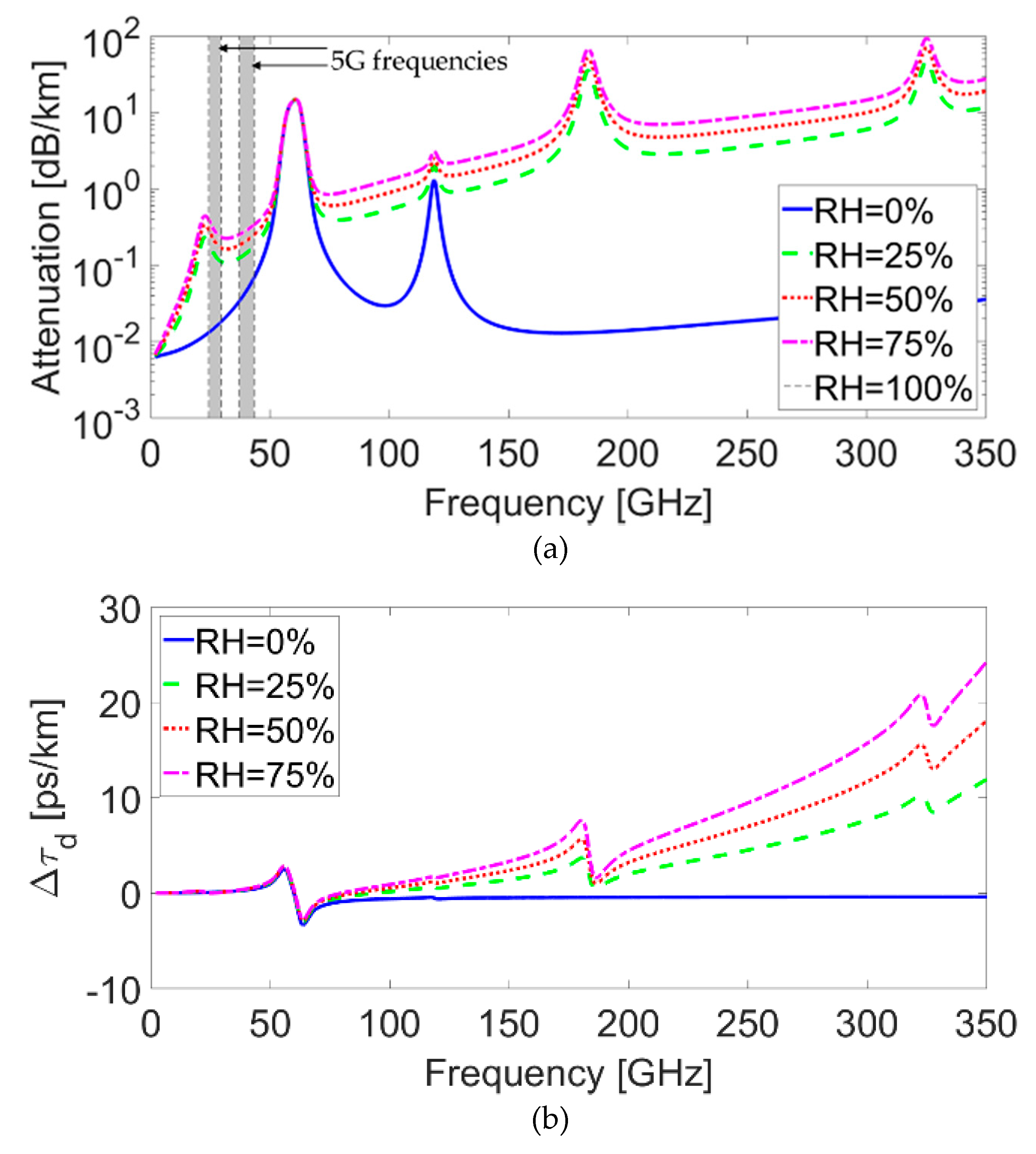
The transmission characteristics of the atmosphere are shown in Figure 1. In this example, graphs are drawn for several values of relative humidity (RH = 0%, 25%, 50%, 75%, and 100%) at sea level, assuming clear skies and no fog or rain. The attenuation factor, in dB/km, is drawn in Figure 1a, revealing absorption peaks at 22 and 183 GHz, where the resonance absorption of water (H2O) occurs; as well as absorption peaks at 60 and 119 GHz, due to the absorption resonances of oxygen (O2) [46,47,48]. A minimum attenuation is obtained at atmospheric transmission “windows” in the Ka- (35 GHz) and W-bands (94 GHz), as well in the vicinity of 130 and 220 GHz [37]. The gray bands represent the spectrum allocated for the 5G. In Figure 1b, we show the incremental group delay (in ps/km) caused by the phase variation in the frequency. The atmospheric transfer characteristics can be calculated for any value of the relative humidity (RH).
When carrying out a link budget, the atmospheric attenuation must be taken into account. In millimeter wave links, the antennas are usually directive, resulting mainly in line-of-sight (LOS) paths. When a transmitter (T; with an effective isotropic radiated power ()) and an interferer (I; with ) transmit a signal to a receiver in their LOS (see Figure 2), the corresponding power from the transmitting station is as follows:
and from the interferer station, it is as follows:
where is the receiver antennas gain, is the wavelength of the transmitted signal (c is the speed of light, f is the frequency), and are the distances between the transmitter or interferer to the receiver, respectively, and is the power attenuation factor caused by the atmospheric medium. The signal to interference power ratio at the receiver site is given by the following:
3. Error Rate Degradation in the Presence of Co-Channel Interference
Co-channel interference occurs between two transmitters that are using the same frequency. The co-channel interference can severely affect the performance of the symbol error rate (SER). In this section, the SER performance properties of the CE-MTO and the CE-OFDM in the presence of co-channel interference are studied.
The signal arriving at the receiver from the transmitter is a constant envelope phase-modulated waveform. Its complex amplitude at baseband is given by the following [25]:
where and Ac is the (constant) signal envelope. is the information-bearing message phase. Assuming an in-band interference, its respective complex amplitude is as follows:
with the power given by the variance, as follows:
where we define SIR as the signal to interference power ratio at the receiver site, as in Equation (3). The interfering signal phase, , is a stochastic process that is uniformly distributed . Both the signal and interference are received simultaneously, resulting in a composite waveform, written as follows:
where its phase is as follows:
Note that when , the resulted phase is , equal to that of the required signal, as expected. In order to calculate the interference component in the phase, we assume . In this case, the phase fluctuation due to the interferer is as follows:
Further analysis considers the detection of orthogonal modulation techniques (CE-OFDM [25] and CE-MTO [26] techniques). In the receiver (see Figure 3), after an analog to digital conversion, the samples, , are sent to the phase demodulator. The output of the phase demodulator in the continuous-time presentation is , where is the phase interference component given by Equation (9). The amplitude is kept constant by a limiter. A set of matched filters calculate the correlations, as follows:
where , is the modulation index, and is a constant used to normalize the variance of the resulted phase, namely: , where M is the pulse-amplitude modulation (PAM) constellation, is the N real valued data symbols, and is the discrete orthogonal waveforms. In the CE-OFDM technique, is the orthogonal subcarriers’ quadrature components, while in CE-MTO is the orthogonal series generated by the Hadamard matrix. is the signal component, as follows:
where , and for the CE-MTO case, and , where is the number of chips contained in the orthogonal waveforms, . For the CE-OFDM case, and , where is the number of points in the inverse discrete Fourier transformation (IDFT). The interference component in Equation (10) is as follows:
As is the independent random values, the sum of Equation (12) makes approximately Gaussian, having . Based on the literature [25], we may approximate SER as follows:
where in our case, we have the following:
The substitution of Equation (6) in Equation (14), and and d in Equation (13), results, for both CE-MTO and CE-OFDM, in the following:
A comparison is made between the analytical results obtained using Equation (15) and those obtained from simulations of the CE-MTO and the CE-OFDM demodulation in the presence of external interference. Figure 4 shows the graphs of the SER as a function of the SIR. The correlations between the graphs are revealed. The graphs were drawn assuming chips for each of the N = 14 orthogonal waveforms. Several PAM constellation orders, M = 4, 8, and 16, wre considered. In order to keep the bandwidth restrained, the modulation index is set to .
4. Performance of AWGN Channel in the Presence of CCI
In the presence of additive white Gaussian noise, , in addition to the interference (see Figure 3), the received signal can be written as follows:
Due to the fact that and are independent random processes, that is, , where the AWGN standard deviation is based on the following [26]:
Here, is the energy per bit of the transmitted signal and is the power spectral density (PSD) of the AWGN. In order to calculate the SER analytical expression of this new scenario, the expression of (13) is used, leading to:
A comparison is made between the analytical results obtained using Equation (18) and the simulation results of the CE-MTO and the CE-OFDM techniques in the presence of external interference and AWGN. Figure 5 shows the simulated results for the SER as a function of the . It is noticeable that there is a high correlation between the simulated results for both modulation techniques (CE-OFDM and CE-MTO).
The graphs in Figure 5 have been created for orthogonal waveforms, each containing chips. The PAM constellation order is M = 4 and the modulation index is kept at . The signal to interference power ratio is assumed to be SIR = 15 dB. The “Analytical AWGN only” curve refers to the analytical expression obtained in our previous work [26] in Equation (21) for the case of the AWGN channel only. The “Analytical Interference only” and the “Analytical Interference and AWGN” curves refer to Equations (15) and (18), respectively. Figure 5 shows that for the case of SIR = 15 dB, M = 4, and , the SER for the “Analytical Interference only” is approximately equal to 0.025. Please note the “Analytical AWGN only” and the “Analytical Interference only” curves function as an asymptote for the “Simulated” and “Analytical Interference and AWGN” graphs in which the interference and AWGN exists.
5. Results for Different CCI Scenarios
The simulation results for the different CCI scenarios are presented in the following. First, it is assumed that the interferer transmits at the very same frequency as the required transmission. Then, a frequency shift, , is introduced to the interferer carrier.
The analytical Equation (18) for the SER in the presence of interference and AWGN depends on the signal to interference (SIR) power ratio at the receiver, on the modulation index (), and the constellation order (M). The case when the carrier frequencies of the transmitter and the interferer are identical is studied. Note that for Figure 6, the “Analytical AWGN only” curve refers to the situation where the PAM constellation order is M = 4 and the modulation index is . In Figure 6a, we show the dependence on the SIR parameter. As expected, a higher SIR results in a lower SER. Figure 6b shows the SER dependence on the modulation index, . As the value of is increased, the SER decreases. Finally, Figure 6c demonstrates the dependence on the constellation M. Smaller constellations show a better performance.
Interferer shift in frequency results in phase , where is the difference in carrier frequencies. Figure 7 presents the spectrum of the CE-OFDM, CE-MTO, and the CW interference. Note that for the CE-MTO, is the time duration of a series “chip”, while for the CE-OFDM, , where N is the number of subcarriers. The inspection of Figure 7 reveals that the CE-MTO spectrum is null for the = integer. The interference is located at . Comparing the two modulation techniques reveals a slight difference between the spectrum of the CE-OFDM and that of the CE-MTO.
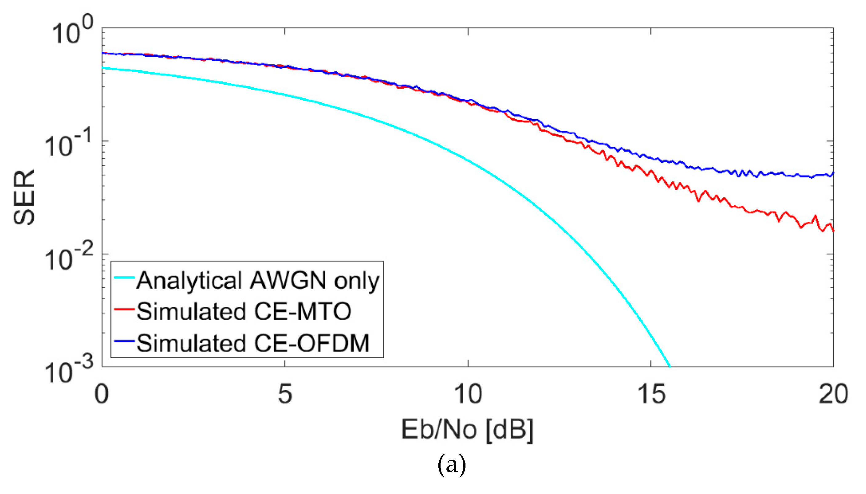
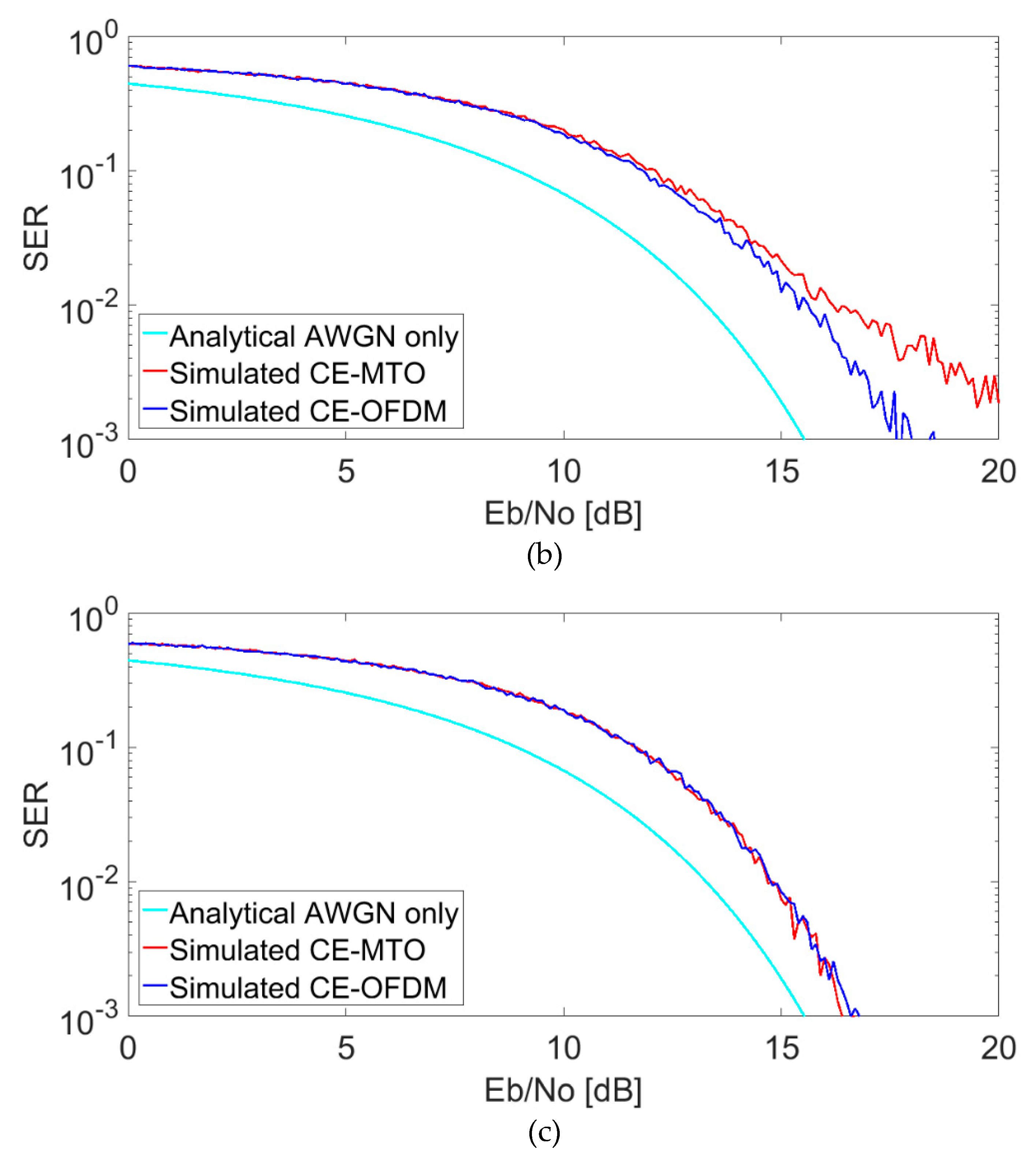
Figure 8a–c shows the graphs of the SER as a function of . The results in Figure 8a–c have been obtained for orthogonal waveforms of chips. The order constellation is M = 4 and the modulation index is . It is assumed that the signal to interference power ratio is SIR = 15 dB for different frequency shift values, . In Figure 8a, where , the performance of CE-MTO is revealed to be better than that of CE-OFDM. However, in Figure 8b, where , the CE-OFDM demonstrates a better performance than that of CE-MTO. The curves in Figure 8c refer to . In this scenario, the performance of CE-MTO and that of CE-OFDM are identical. The results obtained in Figure 8a–c are as expected when examining the spectrum as given in Figure 7.
6. Summary and Conclusions
Small PAPR modulation schemes are being used for better power efficiency. In CE-OFDM, the carrier is phase-modulated with the OFDM signaling to generate a constant envelope waveform. CE-MTO is a new suggested technique for constant envelope modulation, which is based on orthogonal waveforms in the time domain, and with the implementation expected to be simpler than that of the CE-OFDM. An analytical expression for the SER performance degradation caused by the co-channel interference in different scenarios is presented. It is shown that the SER decreases in the presence of interference when the modulation index is increased. The SER grows the higher the constellation order.
Author Contributions
Conceptualization, Y.P. and M.P.; Formal analysis, Y.B.; Investigation, Y.B.; Writing – original draft, Y.B.; Writing – review & editing, Y.P. and M.P.
Funding
This research received no external funding.
Conflicts of Interest
The authors declare no conflict of interest.
References
- Almeida, M.P.; Vargas, C.E.O.; Tamo, A.; Mello, L.S. Interference simulation between 5G and GSO–NGSO networks at 27–30 GHz range. In Proceedings of the 2019 IEEE-APS Topical Conference on Antennas and Propagation in Wireless Communications (APWC), Granada, Spain, 9–13 September 2019; pp. 202–205. [Google Scholar]
- Cianca, E.; Rossi, T.; Yahalom, A.; Pinhasi, Y.; Farserotu, J.; Sacchi, C. EHF for Satellite Communications: The New Broadband Frontier. Proc. IEEE 2011, 99, 1858–1881. [Google Scholar] [CrossRef]
- Lutz, E.; Bischl, H.; Ernst, H.; Giggenbach, D.; Holzbock, M.; Jahn, A.; Werner, M. Development and Future Applications of Satellite Communications. In Emerging Location Aware Broadband Wireless Ad Hoc Networks; Ganesh, R., Kota, S.L., Pahlavan, K., Agustí, R., Eds.; Springer: Boston, MA, USA, 2004. [Google Scholar]
- Etinger, A.; Balal, N.; Litvak, B.; Einat, M.; Kapilevich, B.; Pinhasi, Y. Non-Imaging MM-Wave FMCW Sensor for Pedestrian Detection. IEEE Sens. J. 2014, 14, 1232–1237. [Google Scholar] [CrossRef]
- Yang, X.; Yang, J. A research on millimeter wave LFMCW radar for airfield object imaging. Int. J. Infrared Millim. Waves 2001, 22, 247–253. [Google Scholar] [CrossRef]
- Lin, S.K. Microwave and Millimeter-Wave Remote Sensing for Security Applications. Remote Sens. 2013, 5, 367–373. [Google Scholar] [CrossRef] [Green Version]
- Peng, S.S.; Wu, L.; Ying, X.H. A Receiver in a Millimeter Wave Radiometer for Atmosphere Remote Sensing. Int. J. Infrared Millim. Waves 2009, 30, 259–269. [Google Scholar] [CrossRef]
- Byeon, C.W.; Park, C.S. Low-cost compact millimeter-wave antenna-in-package for short-range wireless communications. Microw. Opt. Technol. Lett. 2017, 59, 329–333. [Google Scholar] [CrossRef]
- Lin, W.; Chen, J.; Zhu, Y.; Kong, F.; Xu, J.; Kuai, L.; Yu, C.; Yan, P.; Hong, W. Wide band compact rf receiver for millimeter wave 5g mobile communication. In Proceedings of the 2016 IEEE International Conference on Ubiquitous Wireless Broadband (ICUWB), Nanjing, China, 16–19 October 2016; pp. 1–4. [Google Scholar]
- Balal, Y.; Pinhasi, Y. Atmospheric effects on millimeter and sub-millimeter (THz) Satellite Communication Paths. J. Infrared Millim. Terahertz Waves 2019, 40, 219–230. [Google Scholar] [CrossRef]
- Antes, J.; Kallfass, I. Performance Estimation for Broadband Multi-Gigabit Millimeter- and Sub-Millimeter-Wave Wireless Communication Links. IEEE Trans. Microw. Theory Tech. 2015, 63, 3288–3299. [Google Scholar] [CrossRef]
- Balal, N.; Pinhasi, G.A.; Pinhasi, Y. Atmospheric and Fog Effects on Ultra-Wide Band Radar Operating at Extremely High Frequencies. Sensors 2016, 16, 751. [Google Scholar] [CrossRef]
- Rappaport, T.S.; Sun, S.; Mayzus, R.; Zhao, H.; Azar, Y.; Wang, K.; Wong, G.N.; Schulz, J.K.; Samimi, M. Millimeter Wave Mobile Communications for 5G Cellular: It Will Work! IEEE Access 2013, 1, 335–349. [Google Scholar] [CrossRef]
- Nordrum, A.; Clark, K. Everything you need to know about 5G. In IEEE Spectrum Magazine; Institute of Electrical and Electronic Engineers: Piscataway, NJ, USA, 2019. [Google Scholar]
- Zhu, J.; Wang, Z.; Li, Q.; Chen, H.; Ansari, N. Mitigating Intended Jamming in mmWave MIMO by Hybrid Beamforming. IEEE Wirel. Commun. Lett. 2019, 8, 1617–1620. [Google Scholar] [CrossRef]
- Hoffman, C. What is 5G, and how fast will it be? In How-To Geek website. How-To Geek LLC; Retrieved: 23 February 2019; Available online: https://www.howtogeek.com/340002/what-is-5g-and-how-fast-will-it-be/ (accessed on 3 December 2019).
- Chen, H.; Shao, H.; Chen, H. Angle-range-polarization-dependent beamforming for polarization sensitive frequency diverse array. EURASIP J. Adv. Signal Process. 2019, 2019, 23. [Google Scholar] [CrossRef] [Green Version]
- Zhou, W.; Chen, H.; Lam, W.H. Optimality of beamforming condition for multiple antenna systems with mean feedback. J. Wirel. Commun. Netw. 2011, 2011, 160. [Google Scholar] [CrossRef] [Green Version]
- Miller, S.L.; O’Dea, R.J. Peak power and bandwidth efficient linear modulation. IEEE Trans. Commun. 1998, 46, 1639–1648. [Google Scholar] [CrossRef]
- Ochiai, H. Power efficiency comparison of OFDM and single-carrier signals. Proc. IEEE VTC 2002, 2, 899–903. [Google Scholar]
- Wulich, D. Definition of efficient PAPR in OFDM. IEEE Commun. Lett. 2005, 9, 832–834. [Google Scholar] [CrossRef]
- Yixuan, H.; Su, H.; Shiyong, M.; Qu, L.; Dan, H.; Yuan, G.; Rong, S. Constant envelope OFDM RadCom fusion system. EURASIP J. Wirel. Commun. Netw. 2018, 2018, 104. [Google Scholar]
- Qian, R.; Jiang, D.; Fu, W. Digital constant-envelope modulation scheme for radar using multicarrier OFDM signals. IET Signal Process. 2017, 11, 861–868. [Google Scholar] [CrossRef]
- Zou, W.Y.; Wu, Y. COFDM: An overview. IEEE Trans. Broadcast. 1995, 41, 1–8. [Google Scholar] [CrossRef]
- Thompson, S.C.; Ahmed, A.U.; Proakis, J.G.; Zeidler, J.R.; Geile, M.J. Constant envelope OFDM. IEEE Trans. Commun. 2008, 56, 1300–1312. [Google Scholar] [CrossRef]
- Balal, Y.; Pinchas, M.; Pinhasi, Y. Constant Envelope Phase Modulation Inspired by Orthogonal Waveforms. IEEE Commun. Lett. 2016, 20, 2169–2172. [Google Scholar] [CrossRef]
- Jadav, N.K. A Survey on OFDM Interference Challenge to improve its BER. In Proceedings of the 2018 Second International Conference on Electronics, Communication and Aerospace Technology (ICECA), Coimbatore, India, 29–31 March 2018; pp. 1052–1058. [Google Scholar]
- Aladwani, A.; Erdogan, E.; Gucluoglu, T. Impact of Co-Channel Interference on Two-Way Relaying Networks with Maximal Ratio Transmission. Electronics 2019, 8, 392. [Google Scholar] [CrossRef] [Green Version]
- Liolis, K.P.; Panagopoulos, A.D.; Cottis, P.G. Use of cell-site diversity to mitigate co-channel interference in 10-66 GHz broadband fixed wireless access networks. In Proceedings of the 2006 IEEE Radio and Wireless Symposium, San Diego, CA, USA, 17–19 October 2006; pp. 283–286. [Google Scholar]
- Ohwatari, Y.; Miki, N.; Asai, T.; Abe, T.; Taoka, H. Performance of advanced receiver employing interference rejection combining to suppress inter-cell interference in LTE-Advanced downlink. In Proceedings of the 2011 IEEE VTC—Fall, San Francisco, CA, USA, 5–8 September 2011; pp. 1–7. [Google Scholar]
- Sun, S.; Gao, Q.; Peng, Y.; Wang, Y.; Song, L. Interference management through CoMP in 3GPP LTE-Advanced networks. IEEE Wirel. Commun. Mag. 2013, 20, 59–66. [Google Scholar] [CrossRef]
- Kiyani, N.F.; Sridharan, V.; Dolmans, G. Co-Channel Interference Mitigation Technique for Non-Coherent OOK Receivers. IEEE Wirel. Commun. Lett. 2014, 3, 189–192. [Google Scholar]
- Li, T.; Mow, W.-H.; Lau, V.K.N.; Siu, M.; Cheng, R.; Murch, R. Robust joint interference detection and decoding for OFDM-based cognitive radio systems with unknown interference. IEEE J. Sel. Areas Commun. 2007, 25, 566–575. [Google Scholar] [CrossRef]
- Crane, R.K. Propagation phenomena affecting satellite communication systems operating in the centimeter and millimeter wavelength bands. Proc. IEEE 1971, 59, 173–188. [Google Scholar] [CrossRef]
- Crane, R.K. Fundamental limitations caused by RF propagation. Proc. IEEE 1981, 69, 196–209. [Google Scholar] [CrossRef]
- Ippolito, L.J. Radio propagation for space communication systems. Proc. IEEE 1981, 69, 697–727. [Google Scholar] [CrossRef]
- Liebe, H.J. Atmospheric EHF window transparencies near 35, 90, 140 and 220 GHz. IEEE Trans. Antennas Propag. 1983, 31, 127–135. [Google Scholar] [CrossRef]
- Bohlander, R.A.; McMillan, R.W. Atmospheric effects on near millimeter wave propagation. Proc. IEEE 1985, 73, 49–60. [Google Scholar] [CrossRef]
- Currie, N.C.; Brown, C.E. Principles and Applications of Millimeter-Wave Radar; Artech House: London, UK, 1987. [Google Scholar]
- Attenuation by atmospheric gases ITU-R P.676-11, 09/2016. Available online: https://www.itu.int/rec/R-REC-P.676-11-201609-I/en (accessed on 3 December 2019).
- Liebe, H.J. An updated model for millimeter wave propagation in moist air. Radio Sci. 1985, 20, 1069–1089. [Google Scholar] [CrossRef] [Green Version]
- Liebe, H.J. MPM—An atmospheric millimeter-wave propagation model. Int. J. Infrared Millim. Waves 1989, 10, 631–650. [Google Scholar] [CrossRef]
- Liebe, H.J.; Manabe, T.; Hufford, G.A. Millimeter-wave attenuation and delay rates due to fog / cloud conditions. IEEE Trans. Antennas Propag. 1989, 37, 1617–1623. [Google Scholar] [CrossRef]
- Liebe, H.J.; Hufford, G.A.; Manabe, T. A model for the complex permittivity of water at frequencies below 1THz. Int. J. Infrared Millim. Waves 1991, 12, 659–675. [Google Scholar] [CrossRef]
- Pinhasi, Y.; Yahalom, A.; Pinhasi, G.A. Propagation Analysis of Ultra-Short Pulses in Resonant Dielectric Media. J. Opt. Soc. Am. B 2009, 26, 2404–2413. [Google Scholar] [CrossRef]
- van Vleck, J.H. The absorption of microwaves by oxygen. Phys. Rev. 1947, 71, 413–424. [Google Scholar] [CrossRef]
- Rosenkranz, P.W. Shape of the 5 mm oxygen band in the atmosphere. IEEE Trans. Antennas Propag. 1975, 23, 498–506. [Google Scholar] [CrossRef]
- Liebe, H.J.; Rosenkranz, P.W.; Hufford, G.A. Atmospheric 60 GHz oxygen spectrum: New laboratory measurements and line parameters. J. Quant. Spectrosc. Radiat. Transf. 1992, 48, 629–643. [Google Scholar] [CrossRef]
Figure 1.
The effect of the atmosphere on (a) attenuation, in dB/km, and (b) group delay increment, in ps/km.
Figure 1.
The effect of the atmosphere on (a) attenuation, in dB/km, and (b) group delay increment, in ps/km.

Figure 2.
Illustration of the signal transmission in the presence of interference. EIRP—effective isotropic radiated power.
Figure 2.
Illustration of the signal transmission in the presence of interference. EIRP—effective isotropic radiated power.
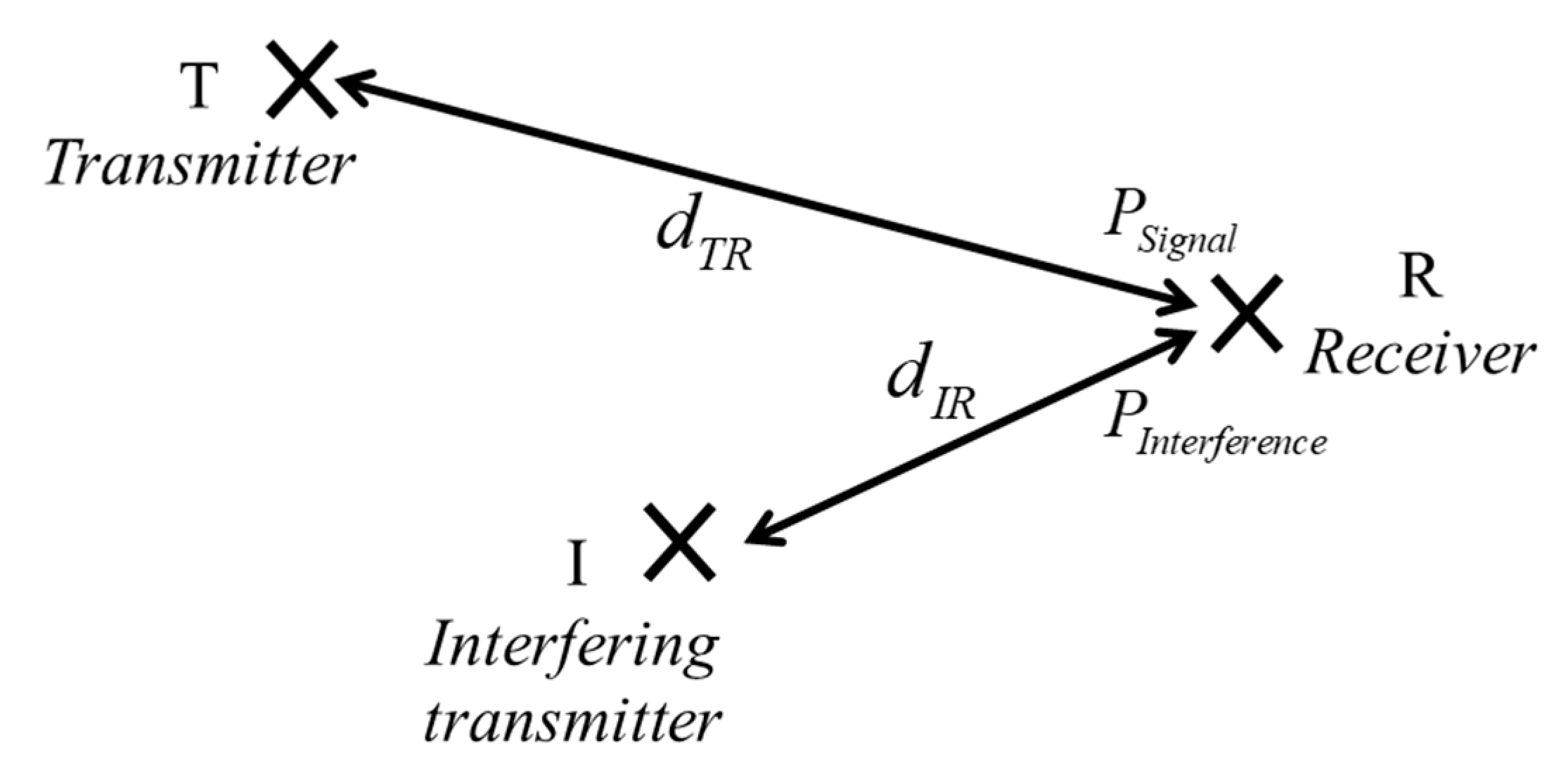
Figure 3.
Constant envelope M-ary time orthogonal (CE-MTO) block diagram.

Figure 4.
Comparison of the symbol error rate (SER) as a function of the signal to interference (SIR) power ratio for the interfered link, , and : (a) M = 4, 8, and 16, , and (b) M = 4, . CE-MTO—constant envelope M-ary time orthogonal; OFDM—orthogonal frequency division multiplexing.
Figure 4.
Comparison of the symbol error rate (SER) as a function of the signal to interference (SIR) power ratio for the interfered link, , and : (a) M = 4, 8, and 16, , and (b) M = 4, . CE-MTO—constant envelope M-ary time orthogonal; OFDM—orthogonal frequency division multiplexing.
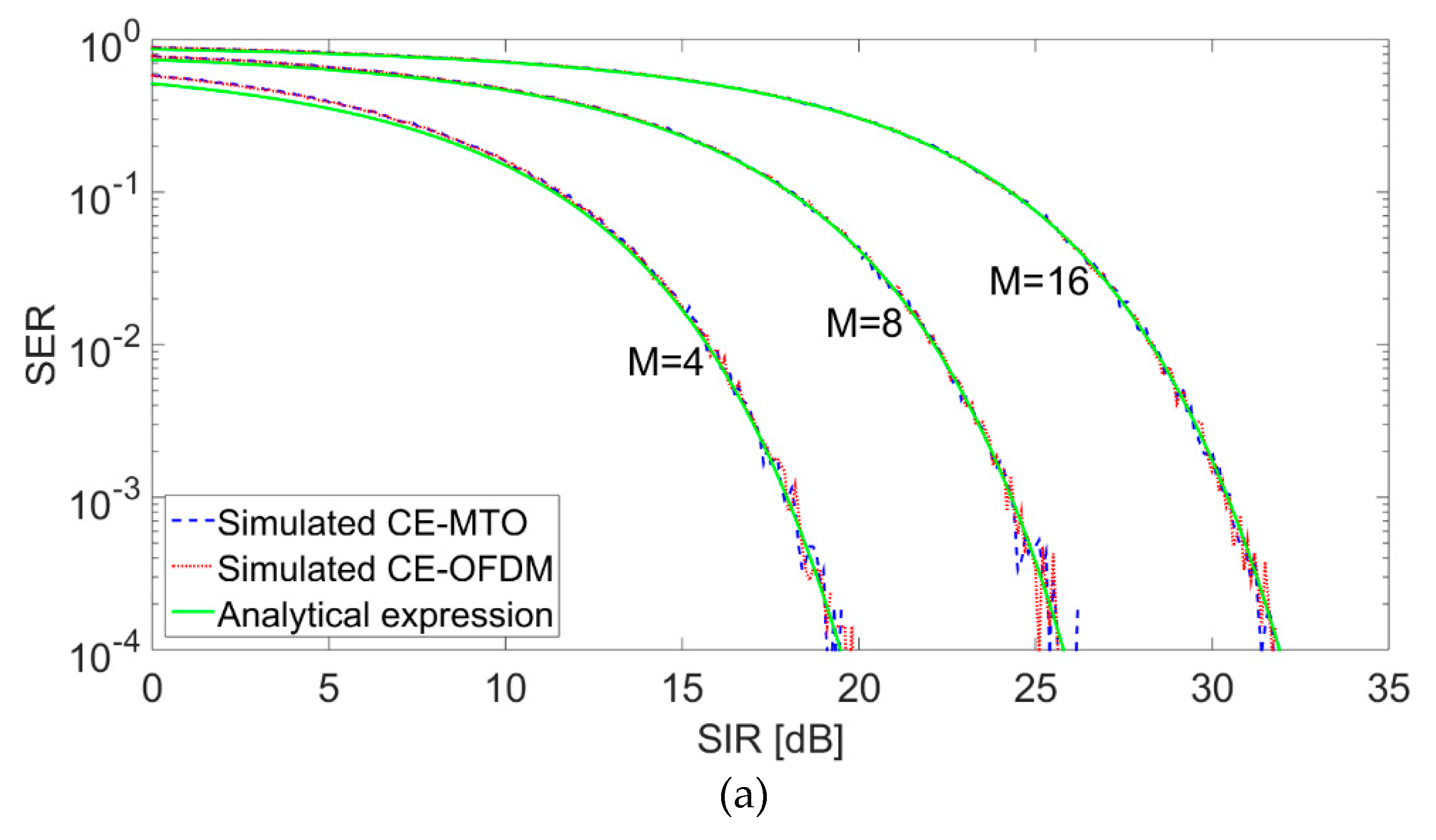
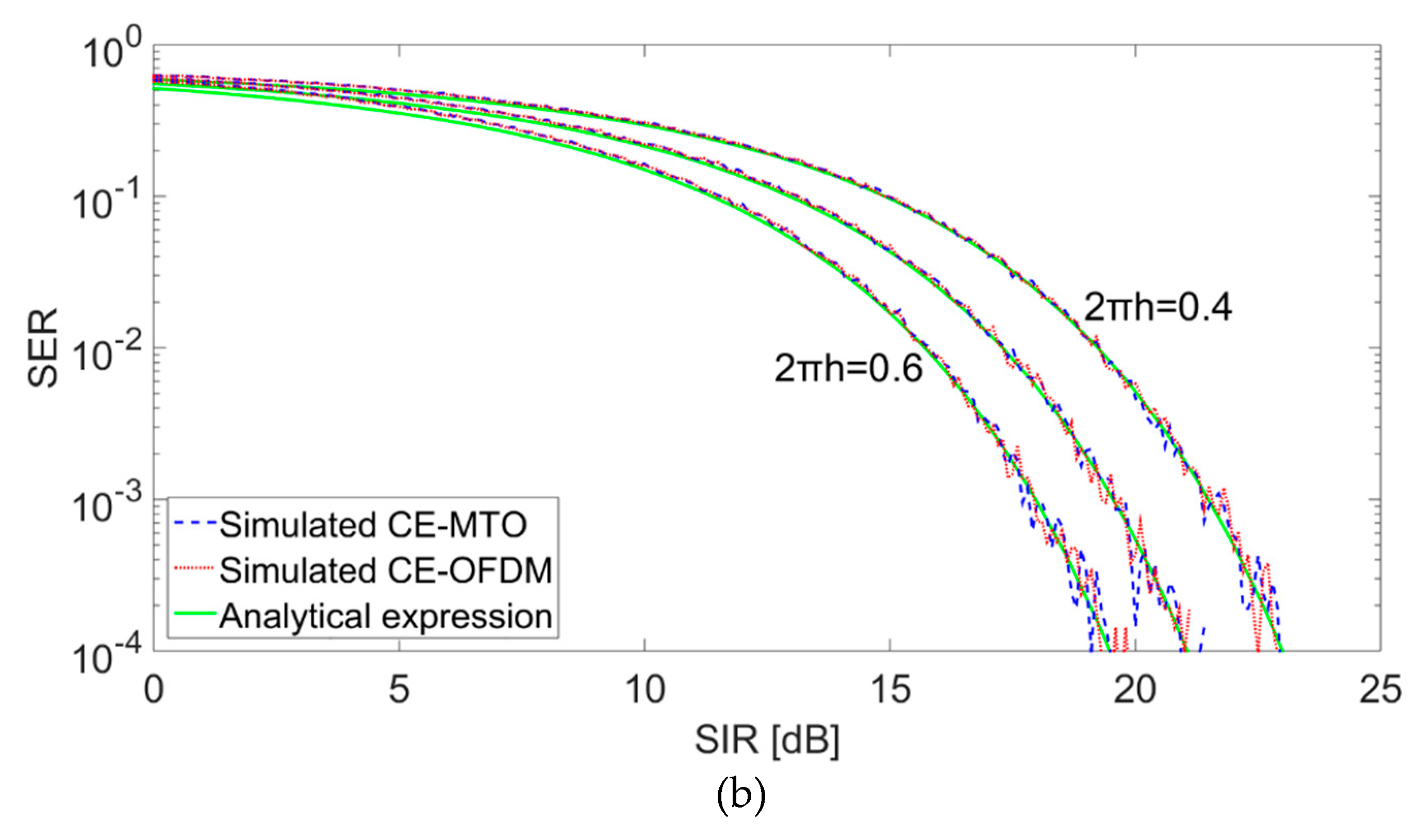
Figure 5.
Comparison of the SER as a function of for interfered link in the present of additive white Gaussian noise (AWGN). , , M = 4, and SIR = 15 dB.
Figure 5.
Comparison of the SER as a function of for interfered link in the present of additive white Gaussian noise (AWGN). , , M = 4, and SIR = 15 dB.
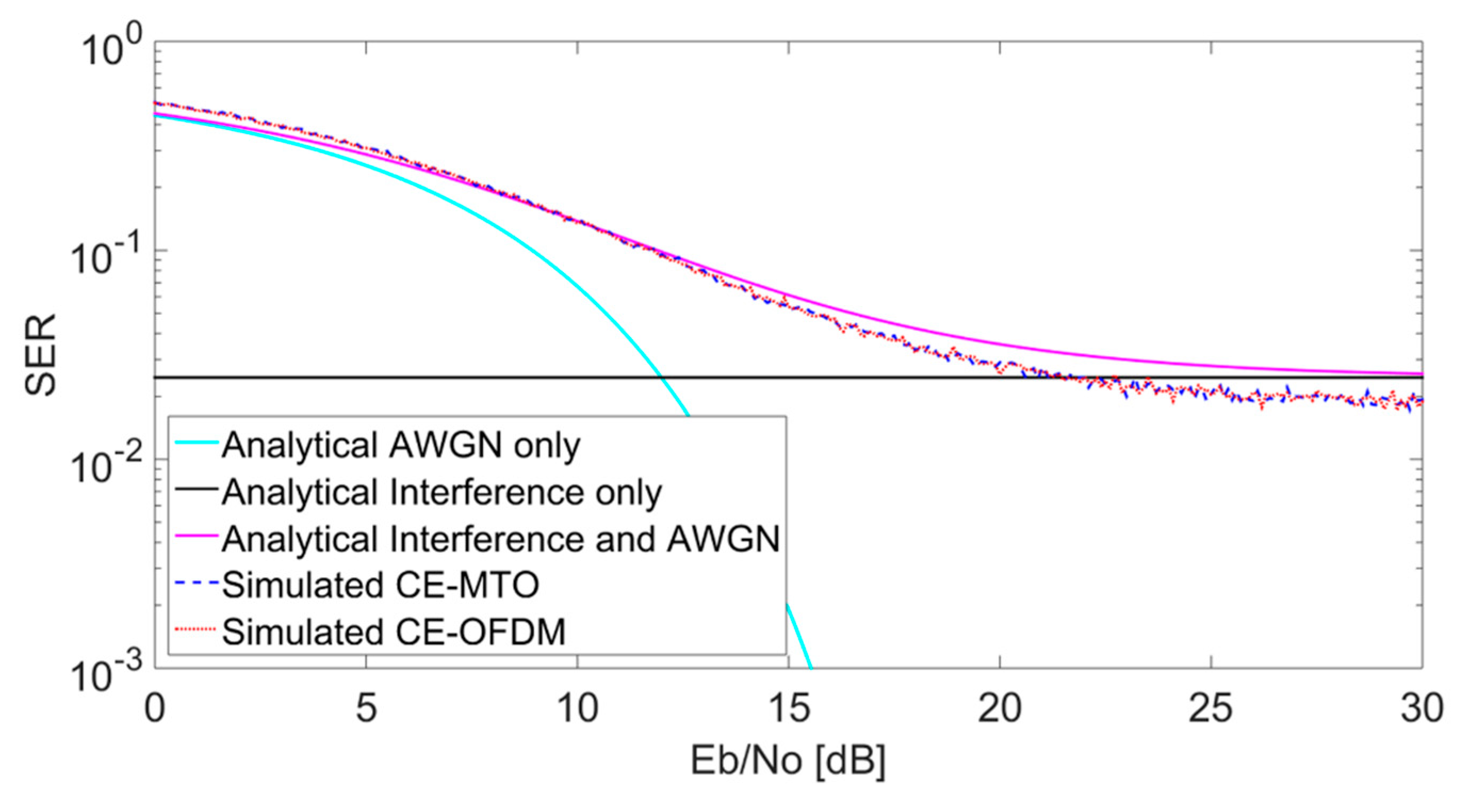
Figure 6.
Comparison of the SER as a function of for the interfered link, , and . (a) M = 4; ; and SIR = 10, 15, and 20 dB. (b) M = 4; SIR = 20 dB; and . (c) ; SIR = 20 dB; and M = 4, 8, and 16.
Figure 6.
Comparison of the SER as a function of for the interfered link, , and . (a) M = 4; ; and SIR = 10, 15, and 20 dB. (b) M = 4; SIR = 20 dB; and . (c) ; SIR = 20 dB; and M = 4, 8, and 16.

Figure 7.
Comparison of the spectrum as a function of the normalized frequency.
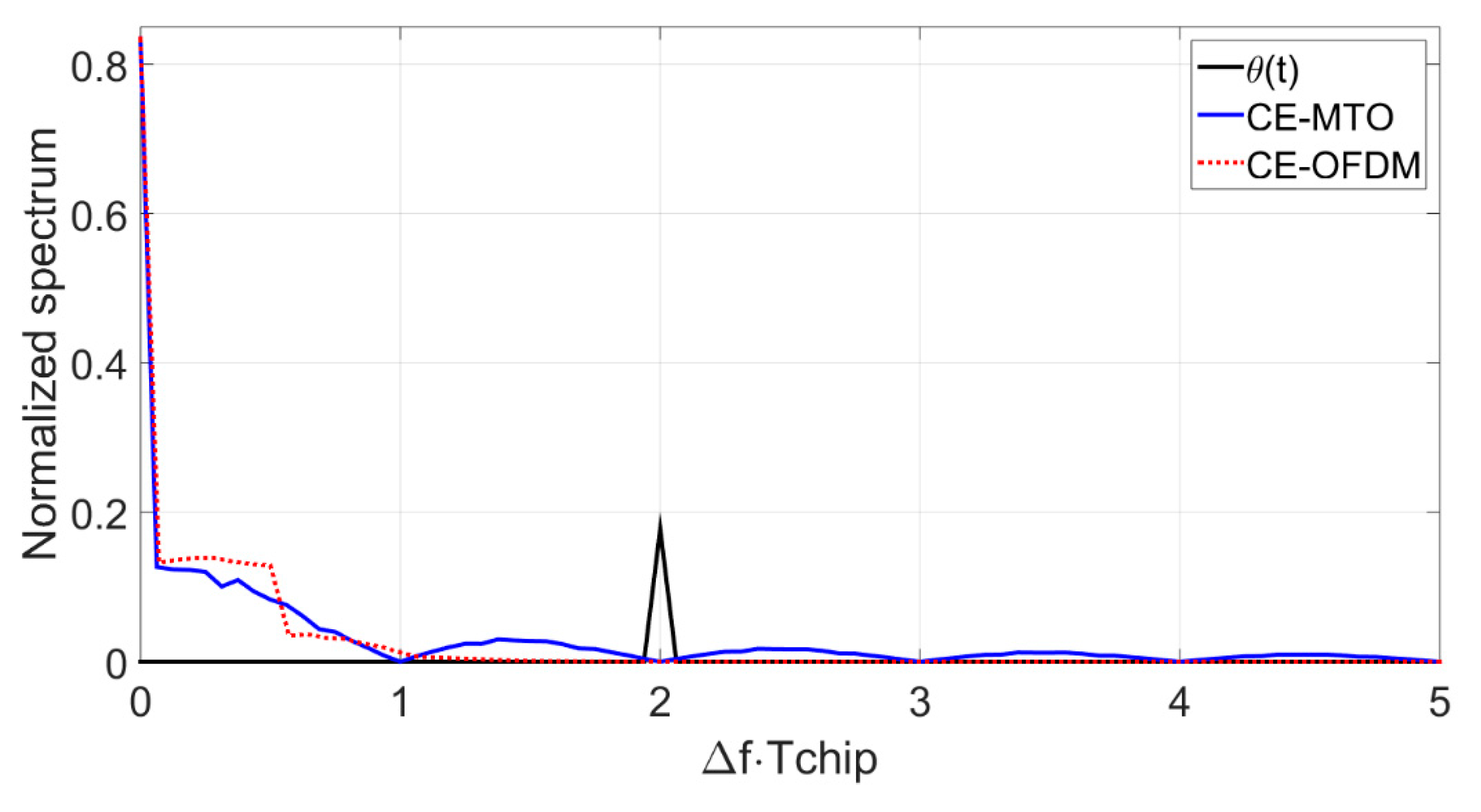
Figure 8.
Comparison of the SER as a function of for the interfered link: (a) , (b) , and (c) .
© 2019 by the authors. Licensee MDPI, Basel, Switzerland. This article is an open access article distributed under the terms and conditions of the Creative Commons Attribution (CC BY) license (http://creativecommons.org/licenses/by/4.0/).
Share and Cite
MDPI and ACS Style
Balal, Y.; Pinchas, M.; Pinhasi, Y. Constant Envelope Modulation Techniques for Limited Power Millimeter Wave Links. Electronics 2019, 8, 1521. https://doi.org/10.3390/electronics8121521
AMA Style
Balal Y, Pinchas M, Pinhasi Y. Constant Envelope Modulation Techniques for Limited Power Millimeter Wave Links. Electronics. 2019; 8(12):1521. https://doi.org/10.3390/electronics8121521
Chicago/Turabian StyleBalal, Yael, Monika Pinchas, and Yosef Pinhasi. 2019. "Constant Envelope Modulation Techniques for Limited Power Millimeter Wave Links" Electronics 8, no. 12: 1521. https://doi.org/10.3390/electronics8121521
Note that from the first issue of 2016, this journal uses article numbers instead of page numbers. See further details here.