Site-Specific Propagation Loss Prediction in 4.9 GHz Band Outdoor-to-Indoor Scenario


School of Environment and Society, Tokyo Institute of Technology, Tokyo 152-8550, Japan
*
Author to whom correspondence should be addressed.
†
Present address: Marvelous Inc., Tokyo 140-0002, Japan.
Electronics 2019, 8(12), 1398; https://doi.org/10.3390/electronics8121398
Submission received: 16 October 2019
/
Revised: 14 November 2019
/
Accepted: 20 November 2019
/
Published: 23 November 2019
(This article belongs to the Special Issue Antennas and Propagation Aspects for Emerging Wireless Communication Technologies)
Abstract
:Owing to the widespread use of smartphones and various cloud services, user traffic in cellular networks is rapidly increasing. Especially, the traffic congestion is severe in urban areas, and effective service-cell planning is required in the area for efficient radio resource usage. Because many users are also inside high buildings in the urban area, the knowledge of propagation loss characteristics in the outdoor-to-indoor (O2I) scenario is indispensable for the purpose. The ray-tracing simulation has been widely used for service-cell planning, but it has a problem that the propagation loss tends to be underestimated in a typical O2I scenario in which the incident radio waves penetrate indoors through building windows. In this paper, we proposed the extension method of the ray-tracing simulation to solve the problem. In the proposed method, the additional loss factors such as the Fresnel zone shielding loss and the transmission loss by the equivalent dielectric plate were calculated for respective rays to eliminate the penetration loss prediction error. To evaluate the effectiveness of the proposed method, we conducted radio propagation measurements in a high-building environment by using the developed unmanned aerial vehicle (UAV)-based measurement system. The results showed that the penetration loss of direct and reflection rays was significantly underestimated in the ray-tracing simulation and the proposed method could correct the problem. The mean prediction error was improved from 7.0 dB to −0.5 dB, and the standard deviation was also improved from 8.2 dB to 5.3 dB. The results are expected to be utilized for actual service-cell planning in the urban environment.
1. Introduction
Owing to the widespread use of various application services such as video streaming and cloud services, which are accompanied by the advancement of mobile terminals, user traffic in cellular networks is rapidly increasing. Thus, for efficient radio resource usage, service-cell planning is an important issue. In particular, cell planning becomes complex in urban areas because many users are also inside high buildings, which are sometimes higher than the base stations (BSs) as shown in Figure 1. Therefore, three-dimensional (3D) service-cell planning is considered in those areas [1].
Knowledge of the propagation loss characteristics in the outdoor-to-indoor (O2I) environment is important for this purpose. To clarify the building entry loss (BEL) characteristics, radio propagation measurements were conducted by up to the 2 GHz band [2,3], 3.5 GHz band [4], 5 GHz band [5,6], 8 GHz band [7], 10 GHz band [8], and 38 GHz band [9]. It was confirmed that the BEL characteristics changed according to the incident angle of the radio wave to the building. Those statistical characteristics were also adopted in the global standard models such as the COST 231 BEL model [10] and ITU-R P.2109 model [11]. For service-cell planning, it is also needed to predict the propagation loss characteristics in the specific service area. The ray-tracing simulation has been widely utilized for predicting those site-specific propagation channel characteristics [12,13,14]. In a typical O2I scenario in which the incident radio waves penetrated indoors through building windows, the penetration loss was represented by the diffraction loss of rays at the window edges [15,16]. However, there still existed a significant discrepancy between the measurement and the ray-tracing simulation. One reason for the discrepancy is thought to be that other penetration losses occurred also by appurtenances such as window blinds and window fences which are attached to the window. Another reason is that the penetration loss occurred because the Fresnel zones of the radio waves were partially shielded by the window. In [17,18], the physical optics approximation was used to clarify the penetrating wave characteristics by calculating the re-radiation of the electromagnetic wave on the window surface. However, because it was necessary to divide the window surface into the numerous meshes such that the size was smaller than the wavelength of the carrier wave for the calculation, it was not feasible to apply it to the ray-tracing simulation for the site planning from the viewpoint of calculation cost.
In this paper, we proposed the extension method of ray-tracing simulation to take those additional penetration loss effects into the simulation. The method consists of the Fresnel zone shielding loss calculation and the transmission loss calculation by equivalent dielectric plate. We conducted radio propagation measurements in front of a research building in the university campus to evaluate the effectiveness of the proposed method. We developed a radio measurement system using an unmanned aerial vehicle (UAV) to realize the various O2I scenarios where the radio waves penetrated indoors through the window from various arrival angles [19,20,21]. In the measurement, the carrier frequency was the 4.9 GHz band for assuming the low super high frequency (SHF) band communication of the 5G cellular system [22,23]. The contribution of our work was to propose the novel extension method of the ray-tracing simulation to predict the penetration loss in the O2I scenario. We proposed to combine the ray-tracing simulation and the theory of diffraction by small holes [24,25] to include the effect of appurtenances such as window blinds and window fence into the simulation for the first time. We showed the effectiveness of the proposed method through exhaustive radio propagation measurements by using the UAV-based measurement system. The mean prediction error was improved from 7.0 dB to −0.5 dB, and the standard deviation was also improved from 8.2 dB to 5.3 dB by the proposed method.
2. Proposal of Propagation Loss Prediction Method for Outdoor-to-Indoor Scenario
2.1. Proposed Extension Method for Ray-Tracing Simulation
The ray-tracing simulation [12,13,14] has been widely used for the propagation loss prediction in the site-specific environments for service-cell planning. In the simulation, the trajectories of each radio wave, which are called “rays” are traced by calculating the interactions such as reflection, diffraction, and transmission by interactive objects in the environment. Based on the ray optics approximation, all the objects are modeled by large flat polygon surfaces for the calculation. Therefore, the ray-tracing is especially suitable for the radio propagation simulation in built environments. In the simulation, the electric field strength of the received signal E is calculated as follows
Here, we assume that the propagation channel is represented by the superposition of I rays. represents the received electric field strength of ray , is the carrier wavelength, k is the wave-number , is the transmission power, and and are the transmitter (Tx) and receiver (Rx) antenna gains for ray i. The antenna gains are calculated by considering the angle of departure and the angle of arrival of the ray. It is assumed that the ray i suffers the N times reflections, the M times diffractions, and the P times transmissions during the propagation, and it suffered the interaction losses , , and , respectively. The diffraction loss is calculated based on the uniform geometrical theory of diffraction (UTD) [26,27]. is the total propagation length from the -th diffraction point to the m-th diffraction point. The pathgain is the gain by the radio propagation and defined as follows.
Although the ray-tracing simulation can be utilized for the propagation loss prediction in the O2I scenarios, there are several problems. We assume in a typical O2I scenario that the rays penetrate indoors through the building windows as shown in Figure 2. In the existing ray-tracing simulation, the penetration loss is modeled by the diffraction loss at window edges, and no penetration loss is taken into account if the trajectory of ray does not cross the window edges by even a little gap. This calculation has a risk to underestimate the penetration loss, because each ray has its Fresnel zone along the propagation path, and the penetration loss occurs if interactive objects shield the zone [28]. This phenomenon is fundamental to understand various penetration loss characteristics through the window, such as the distance dependency between the window and the indoor station and carrier frequency dependency. In addition, many appurtenances such as window blinds and window fences are attached to the window, and they are also thought to cause further penetration loss. However, taking the influence of those appurtenances into the simulation is not straightforward because of their complex structures, which are far from the assumption of the ray-tracing simulation that the objects are modeled by large flat polygon surfaces. Therefore, the influence of appurtenances has been ignored in the current researches, but it can cause further penetration loss underestimation problem.
In this paper, we propose the extension method of the ray-tracing simulation to take those effects into the penetration loss calculation. In our proposal, we don’t require the fine 3D environment model for the simulation because there is another difficulty to obtaining accurate models in real environments. Because the very detailed electromagnetic simulation has a high calculation cost and it is not suitable for the service-cell planning, we used the simplified calculation method from the simplified model. The difference between the existing ray-tracing simulation and the proposed method is shown in Figure 2. The proposed method consists of the Fresnel zone shielding loss calculation and the transmission loss calculation by equivalent dielectric plate. In the proposed method, normal ray-tracing simulation was calculated firstly, and the trajectory of each ray was investigated. Next, the Fresnel zone shielding loss and the transmission loss by appurtenances of ray i were calculated, and those additional losses were added to the electric field strength and pathgain calculation in (1) and (2).
The details for the calculation of and are explained in the next subsection.
2.2. Fresnel Zone Shielding Loss Calculation
In the Fresnel zone shielding loss calculation, the total propagation distance from the previous indoor diffraction point to the window intersection point and the distance from the window intersection point to the next outdoor diffraction point are calculated for ray i as shown in Figure 2 (b). Although it is assumed that the ray originated from the indoor Tx and propagated to outdoor Rx in the figure, the same theory can be applied also if the Tx and Rx positions were opposite because the reciprocity was satisfied. Fresnel radius of the ray at the window intersection point is calculated as follows.
The cross-section of the Fresnel zone on the window plane is calculated by the incident angle of the ray to the window . The cross-section becomes an ellipse with the major axis and minor axis . Next, the shielding ratio of the first Fresnel zone is calculated by considering the cross-section shape of the window. In this paper, to simplify the calculation, we approximate the Fresnel zone shielding loss by the inverse of .
The reason for the simplification is that there is difficulty in obtaining the detailed 3D environment model in real environments, and the rigorous calculation is not always effective regardless of the high calculation cost. Those calculation procedures were performed for all rays except for the rays that diffracted at the window edge. The reason why the diffracted rays were excluded from the calculation is that the Fresnel zone shielding effect of those rays is already included in the diffraction loss calculation. In that case, is set to 1 in (3).
2.3. Transmission Loss Calculation by Equivalent Dielectric Plate
Many appurtenances such as window blinds and window fences are often attached around the window, and they are thought to affect the penetration loss characteristics. However, the calculation of those effects is not straightforward, because their shapes are thought to be a kind of screen but they have a complicated structure in detail, which is quite different from the plane surface that the ray-tracing simulation assumes. Therefore, the calculation method needed to deal with the effect of the structure in the ray-tracing based simulation. In this paper, we assumed that those screen structures were able to be modeled by the metal plates with periodically perforated small holes, and we calculate the transmission loss by regarding the plate as an equivalent dielectric plate [29,30] based on the theory of diffraction by small holes [24,25]. The calculation model is shown in Figure 3. it is assumed that small round holes are periodically perforated in the metal plate. is the thickness of the plate, and the hole spacing a and the hole diameter d are thought to be enough smaller than the carrier wave wavelength . We consider that the transverse electric (TE) wave arrives from the incident angle . In the case, it was thought that the magnetic dipole was induced on each small circular hole by the incident magnetic field .
Here, is the permeability of the free space. Another magnetic dipole was induced also on the opposite side of the plate by the magnetic field, which passed through the hole. The attenuation coefficient by the hall was analyzed numerically by [31], and it is known that is calculated as follows in case of the round hall.
The electric field on the opposite side of the plate was obtained by calculating the re-radiation of the electric field by the induced magnetic dipoles. Here, we approximated the electric field by assuming that the magnetic dipoles on each hole were not coupled, and the phases of radiated waves were the same from the far-field assumption. In that case, the electric field on the opposite side was thought to be proportional to the hole density , and was calculated as follows in the far-field condition.
Here, S is the area of the plate, is the permittivity of the free space, is the angular frequency, r is the distance between the mobile station (MS) and the BS, and is the speed of light. We used the relation . The electric field when there was no obstacle between the MS and BS can be obtained by calculating the re-radiation of the electric field by the equivalent source on the plane by the Huygens–Fresnel principle.
The transmission loss can be calculated from the ratio of and .
(11) was slightly modified to improve the estimation accuracy in case of large incident angle in [29], and finally, the total transmission loss of ray i [dB] defined as follows.
The transmission loss characteristics by a variety of screen structures are modeled by the parameters such as the plate thickness, the hole spacing, and the hole diameter. It might be possible to substitute the different types of screens by the periodically perforated plates also. The parameterizing method of the different types of screens by the equivalent periodically perforated plates will be future work.
3. 4.9 GHz Band Radio Measurement for Penetration Loss Characteristics from Window
3.1. Radio Measurement System Using UAV
The diagram of the developed radio propagation measurement system is shown in Figure 4. The radio transceiver was implemented on a universal software radio peripheral (USRP) N210 [32], which is one of the commercial SDR platforms. In the measurement, the Tx was set indoors, and the Rx was mounted on the UAV. These were regarded as the indoor MS and virtual outdoor BS, respectively. The Tx-side USRP was controlled by a laptop personal computer (PC) and sends the continuous wave (CW) signal. The Rx recorded the instantaneous narrowband receiving power continuously during the measurement. The Rx-side USRP was controlled by Raspberry Pi [33], which was a single-board computer to reduce the payload. The photograph of the UAV station is shown in Figure 5. The total payload was less than 1 kg, and it could be operated using the portable battery of the UAV. The total dimensions of the system including the UAV were less than 60 cm × 60 cm × 50 cm, and it was usable for various BS placements in various measurement environments. Since the flight course of the UAV was not correctly controlled as planned because of natural disturbances such as wind conditions, it is crucial to know its actual flight trajectory for the data analysis. The UAV also recorded several sensor outputs as the flight data. We calculated the UAV height from the barometer data, the horizontal position from the GPS data, and the direction from the gyroscope data. Since the measurement and flight data were associated with the time stamp information, it was possible to trace the 3D position of the UAV and obtain the receiving power at each position by the post data processing.
In the data analysis, the average receiving power of the q-th snapshot was defined by 3D moving averaging as follows:
where, is the UAV position of the q-th snapshot, and is the 3D window length. (14) gives the average receiving power inside the rectangular prism that size is . The actual window length values that was used for the experiment is shown in Table 1.
3.2. Measurement Method
Radio measurements were conducted in the 4.9 GHz band to investigate penetration loss characteristics from various incident angle conditions from the outdoor BS to the indoor MS through a building window. The measurement map and photos are shown in Figure 6. The Tx was set indoors, and the Rx was mounted on the UAV. These were regarded as the indoor MS and virtual outdoor BS, respectively, because the reciprocity was satisfied in the measurement. The indoor MSs were fixed at three positions marked MS1, MS2, and MS3 in the conference room on the sixth floor. The distances of the positions from the window were 0.4 m, 2.4 m, and 4.4 m, respectively. As shown in Figure 6, a steel window fence was attached outside the window. The window fence consisted of the thick balustrade and the meshed screen with small holes. The floor height was 20 m from the ground, and the MS antenna height was 1.7 m from the floor. The outside measurement areas were grass fields in front of the buildings. The horizontal measurement courses were set parallel to the building external walls, and the course length was 20 m. The measurement plane was 20 m horizontal length by 15 m height in front of the buildings. We obtained the propagation loss profile on the plane to investigate the penetration loss characteristics from various BS positions.
To simplify the measurement procedure, we divided the horizontal course into 2 m intervals. At each measurement point, the BS ascended to approximately 15 m in height and subsequently descended slowly. By repeating the same procedure at all points, the propagation loss characteristics of the 20 m by 15 m measurement plane in front of the building were obtained. Other measurement parameters are summarized in Table 1. Before the measurement, the measured value of the Rx was calibrated by connecting the RF cables between the Tx and the Rx directly. The UAV position was obtained from the flight log, and the moving average of the receiving power was calculated as shown in (14) to eliminate the multi-path fading effect. The antenna radiation pattern of the UAV station was measured in an anechoic chamber in advance, and the antenna elevation directivity effect was canceled from the measured data based on the grazing angle.
4. Penetration Loss Prediction Results
4.1. Ray-Tracing Simulation Method
The ray-tracing simulation was performed to evaluate the prediction performance of the proposed method. The 3D environment model which was created by Sketch-up is shown in Figure 7. The concrete, the plasterboard, and the steel were selected as the building materials. To simplify the model, all the furniture in the room was excluded, and other buildings around the target building were not taken into account. About the window fence, only the balustrade part was included in the model to calculate the diffraction wave at the balustrade.
Raplab software [34] was used for the ray-tracing engine. In the simulation, the method of imaging algorithm [14] was used, and the maximum number of reflections was three, the maximum number of diffractions was one, and the maximum number of transmissions was one. Dipole antennas were applied on both the BS and MS sides. Although the theoretical radiation pattern was used for the indoor MS, the measured pattern was used for the outdoor BS to consider the influence of the UAV frame on the pattern. The elevation radiation pattern of BS measured in an anechoic chamber is shown in Figure 7c. Because the pattern had an upward trend owing to the UAV frame effect, it is thought that the contribution of the reflection waves from the ground was not significant in the measurement. Therefore, the ground reflection waves were not calculated in this simulation.
Firstly, the normal ray-tracing simulation was performed by the above model. Then, the Fresnel zone shielding loss was calculated from the simulation result and the window geometry as explained in Section 2.2. The metal plate with periodically perforated small holes was assumed for the screen part of the window fence, and the equivalent transmission loss was calculated as explained in Section 2.3 if the rays intersected the fence. Other simulation parameters are summarized in Table 2. The normal ray-tracing simulation result and the proposed method were compared to the measurement result, to evaluate the prediction performance.
4.2. Numerical Results
The measurement and simulation results of the MS1 and MS3 settings are summarized in Figure 8 and Figure 9. Figure 8a and Figure 9a show the vertical–horizontal domain receiving power profiles of the measurements. The MS position is also shown for reference. In either MS settings, although the measured receiving power tended to increase as the BS position approached to the MS position, the receiving power in the MS3 setting was much smaller than the result of MS1 because of more severe penetration loss. Figure 8b showe the receiving power prediction result of the ray-tracing simulation. The receiving power was obviously overestimated at most of the BS positions. To clarify the reason for the discrepancy, the schematic propagation routes of the rays in the simulation are shown in Figure 8c. In the MS1 setting, most of the BS positions were under the line-of-sight (LoS) condition because the indoor MS was located close to the window. Therefore, any penetration loss was not considered in that area. Figure 8d presents the receiving power result of the ray-tracing simulation, but all distraction rays were excluded from the calculation. The figure showed that the area where the receiving power was overestimated in Figure 8 a corresponds to the area of Figure 8d. About the reflection and diffraction rays, although the rays reflected from the ceiling of the room were observed in the area marked (A), the receiving power contribution was not significant because this area overlapped with the LoS area. Because no direct and reflection waves were observed the diffraction waves were dominant in the area marked (B). Therefore, the receiving power significantly decreased in the same area in Figure 8a. The receiving power prediction of the proposed method is shown in Figure 8e. The overestimation of receiving power was corrected well in the proposed method by considering the Fresnel zone shielding loss and the transmission loss by equivalent dielectric plate for the direct and reflection rays. The result indicated that the dominant reasons for the penetration loss were the Fresnel zone shielding of the window and the window fence shielding rather than the diffraction at the window edge in this setting. The result showed the effectiveness of the proposed method. The prediction error of the proposed method compared to the measurement is shown in Figure 8f. The positive value means that the prediction of the proposed method was higher than the measurement. The error was relatively higher in the areas where the direct and reflection waves were dominant, but the error was less than ±5 dB in most of the areas.
The same analysis was performed for the MS3 setting. The measurement result and the ray-tracing simulation result are shown in Figure 9a,b. In the simulation, the receiving power was overestimated in the area marked (A) while it was underestimated in the area marked (B). The reason for these discrepancies was analyzed in Figure 9c,d. Because the distance between the indoor MS and the window increased, most of the BS positions were under the non-Line-of-Sight (NLoS) condition. Therefore, the single and double bounce reflections became a more dominant propagation mechanism. By comparing Figure 9a,d, it can be seen that area (A) corresponded to the area that direct and reflection waves were observed like the MS1 setting. No direct and reflection waves were observed when the BS height was about 5 m, and the diffraction waves were dominant in the area. Especially, the receiving power reduced in area (B) because multiple losses owing to the reflections and the diffractions occurred. On the whole, in the ray-tracing simulation, the diffraction waves were tended to be estimated weaker than the measurements. This problem might be because of the issue of the ray-tracing simulation itself or because of the accuracy of the environment model such as the detailed structures and material parameters of the interactive objects. Further detailed analysis will be future work. In the receiving power prediction of the proposed method shown in Figure 9e, the overestimation issue of the receiving power in the area (A) was fairly corrected. However, the underestimation issue in the area (B) remained.
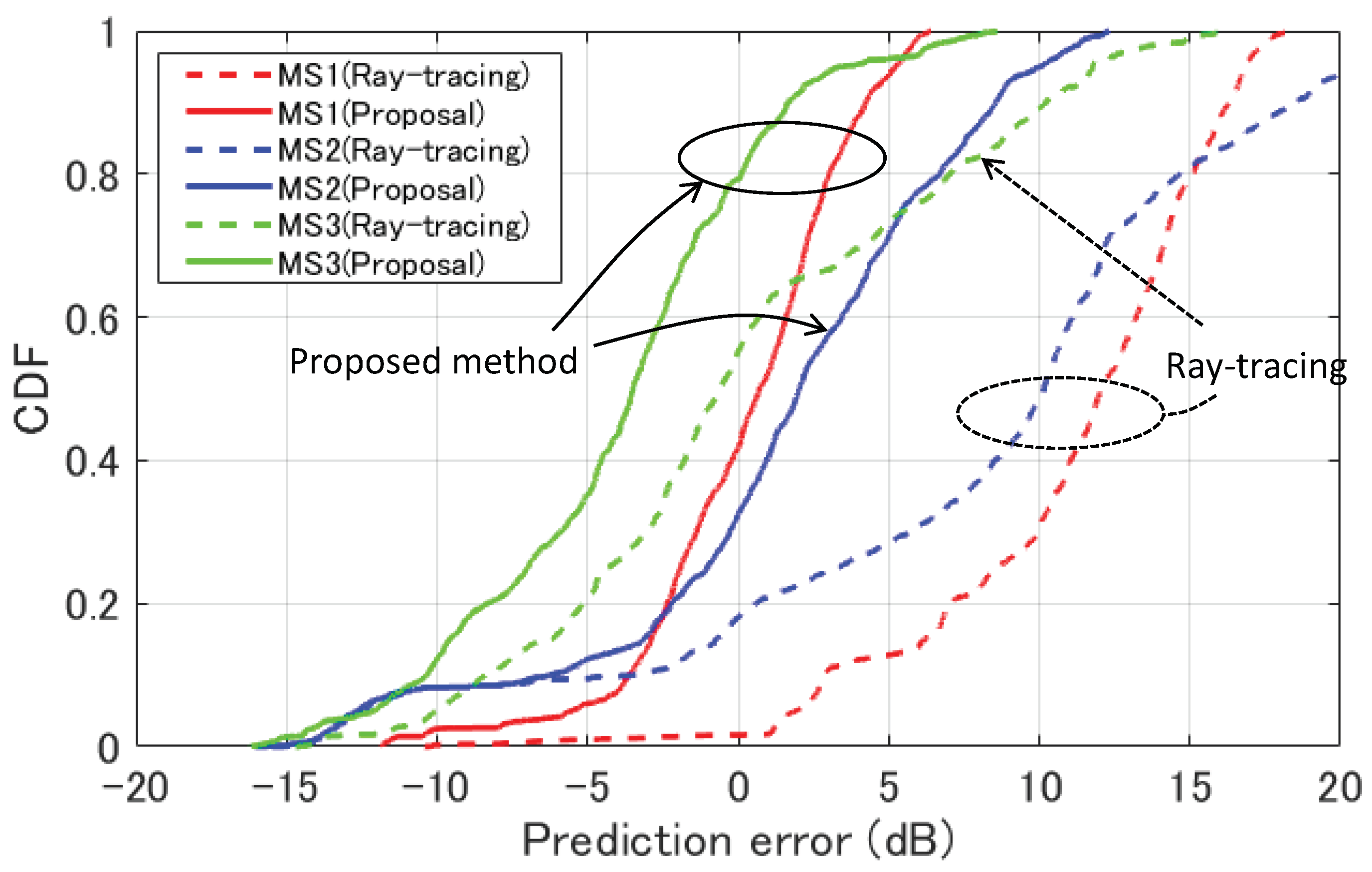
The prediction errors of the ray-tracing simulation and the proposed method are summarized in Figure 10. The data represent the prediction error CDF of all BS positions. The positive error means that the prediction result was higher than the measurement. The mean and the standard deviation of the error is summarized in Table 3. As described in the previous paragraphs, the ray-tracing simulation had the problem of underestimating the penetration loss. The mean errors were 11.1 dB and 8.0 dB in the MS1 and MS2 settings, respectively. Although the mean error was 0.4 dB in the MS3 setting, it does not mean the correct power was predicted. In actuality, the power of direct and reflecting waves was overestimated and the power of diffraction waves was underestimated, and they happened to balance in this environment. In the proposed method, the mean errors were improved to 0.3 dB and 1.5 dB in the BS1 and BS2 settings, respectively, while the error slightly increased in the BS3 setting because of the inaccuracy of diffraction loss estimation. However, the total prediction error was improved from 7.0 dB to −0.5 dB, and the result proved the effectiveness of the proposed method. About the dispersion of error, the standard deviation was also improved from 8.2 dB to 5.3 dB.
The significance of the result is that our proposal is not a kind of predicted offset that increases or decreases the receiving power in the same way. Because the power correction was executed for each ray by considering the physical propagation mechanism, the method is robust enough to be applied to a variety of radio propagation conditions. The utilization of the proposal for the actual service-cell planning is expected to be future work.
5. Conclusions
In this paper, we proposed the extension method of the ray-tracing simulation for a typical O2I scenario in which the incident radio waves penetrate indoors through the building windows. Because only the diffraction loss at window edges is considered in the existing ray-tracing simulation, it has the problem of underestimating the penetration loss. Our proposed method consists of the Fresnel zone shielding loss calculation and the transmission loss calculation by equivalent dielectric plate. In the Fresnel zone shielding loss calculation, the Fresnel zone cross-sections of respective rays on the window plane were evaluated, and the shielding losses were calculated by the shielding ratios of the zones. In the transmission loss calculation by equivalent dielectric plate, we proposed to substitute the screen-type appurtenances such as window blinds and window fences by an equivalent dielectric plate. The transmission loss of the equivalent plate can be calculated based on the theory of diffraction by small holes.
To evaluate the effectiveness of our proposal, we conducted radio propagation measurements in a high-building environment by using the developed UAV based measurement system. The result showed that the penetration losses of direct and reflection rays were underestimated in the ray-tracing simulation. This prediction error became significant as the indoor MS approached the window, and the mean error was 11.1 dB when the distance between the indoor MS and the window was 0.4 m. The total prediction error was 7.0 dB in the ray-tracing simulation. In the proposed method, the mean prediction error was improved to 0.3 dB in that case and the total prediction error was improved to −0.5 dB. The standard deviation of the prediction error was also improved from 8.2 dB to 5.3 dB. The results are expected to be utilized for actual service-cell planning in the urban environment. We found another problem that the diffraction loss was overestimated in the ray-tracing simulation. The solution to the problem will be future work.
Author Contributions
K.S. designed the measurement system and the experiment, and he was in charge of the data analysis and simulation part of the study. Q.F. was in charge of the drone controlling for the experiment. N.K. was in charge of the implementation of radio transceiver on the SDR platform. J.-i.T. supervised the project, and provided advice and support to promote the project.
Funding
This work was supported by the Fujikura foundation and the Support Center for Advanced Telecommunications (SCAT) foundation.
Conflicts of Interest
The authors declare no conflict of interest.
References
- Omote, H.; Miyashita, M.; Yamaguchi, R. Measurement of time-spatial characteristics between indoor spaces in different LOS buildings. In Proceedings of the 2015 International Symposium on Antennas and Propagation (ISAP), Hobart, Australia, 9–12 November 2015; pp. 1–4. [Google Scholar]
- de Jong, Y.L.C.; Koelen, M.H.J.L.; Herben, M.H.A.J. A building-transmission model for improved propagation prediction in urban microcells. IEEE Trans. Veh. Technol. 2004, 53, 490–502. [Google Scholar] [CrossRef]
- Axiotis, D.I.; Theologou, M.E. An empirical model for predicting building penetration loss at 2 GHz for high elevation angles. IEEE Antennas Wirel. Propag. Lett. 2003, 2, 234–237. [Google Scholar] [CrossRef]
- Chee, K.L.; Anggraini, A.; Kaiser, T.; Kurner, T. Outdoor-to-indoor propagation loss measurements for broadband wireless access in rural areas. In Proceedings of the 5th European Conference on Antennas and Propagation (EUCAP), Rome, Italy, 11–15 April 2011; pp. 1376–1380. [Google Scholar]
- Alatossava, M.; Suikkanen, E.; Veli-Matti, J.M.H.; Ylitalo, J. Extension of COST 231 Path Loss Model in Outdoor-to-Indoor Environment to 3.7 GHz and 5.25 GHz. In Proceedings of the 11th International Symposium on Wireless Personal Multimedia Communications, Saariselkä, Finland, 23–27 September 2008; pp. 1–4. [Google Scholar]
- Medbo, J.; Furuskog, J.; Riback, M.; Berg, J.E. Multi-frequency path loss in an outdoor to indoor macrocellular scenario. In Proceedings of the 2009 3rd European Conference on Antennas and Propagation, Berlin, Germany, 23–27 March 2009; pp. 3601–3605. [Google Scholar]
- Okamoto, H.; Kitao, K.; Ichitsubo, S. Outdoor-to-Indoor Propagation Loss Prediction in 800-MHz to 8-GHz Band for an Urban Area. IEEE Trans. Veh. Technol. 2009, 58, 1059–1067. [Google Scholar] [CrossRef]
- Roivainen, A.; Hovinen, V.; Tervo, N.; Latva-aho, M. Outdoor-to-indoor path loss modeling at 10.1 GHz. In Proceedings of the 2016 10th European Conference on Antennas and Propagation (EuCAP), Davos, Switzerland, 10–15 April 2016; pp. 1–4. [Google Scholar] [CrossRef]
- Imai, T.; Kitao, K.; Tran, N.; Omaki, N.; Okumura, Y.; Nishimori, K. Outdoor-to-Indoor path loss modeling for 0.8 to 37 GHz band. In Proceedings of the 2016 10th European Conference on Antennas and Propagation (EuCAP), Davos, Switzerland, 10–15 April 2016; pp. 1–4. [Google Scholar] [CrossRef]
- COST 231. COST Action 231—Digital Mobile Radio Towards Future Generation Systems—Final Report; Office for Official Publications of the European Communities: Luxembourg, 1999. [Google Scholar]
- ITU-R Recommendation P. 2109. Prediction of Building Entry Loss. 2017. Available online: https://www.itu.int/rec/R-REC-P.2109/en (accessed on 21 November 2019).
- McKown, J.W.; Hamilton, R.L. Ray tracing as a design tool for radio networks. IEEE Netw. 1991, 5, 27–30. [Google Scholar] [CrossRef]
- Seidel, S.Y.; Rappaport, T.S. Site-specific propagation prediction for wireless in-building personal communication system design. IEEE Trans. Veh. Technol. 1994, 43, 879–891. [Google Scholar] [CrossRef]
- Costa, E. Ray tracing based on the method of images for propagation simulation in cellular environments. In Proceedings of the Tenth International Conference on Antennas and Propagation (Conf. Publ. No. 436), Edinburgh, UK, 14–17 April 1997; Volume 2, pp. 204–209. [Google Scholar] [CrossRef]
- Rodriguez, I.; Nguyen, H.C.; Sorensen, T.B.; Zhao, Z.; Guan, H.; Mogensen, P. A novel geometrical height gain model for line-of-sight urban micro cells below 6 GHz. In Proceedings of the 2016 International Symposium on Wireless Communication Systems (ISWCS), Poznan, Poland, 20–23 September 2016; pp. 393–398. [Google Scholar] [CrossRef]
- Inomata, M.; Sasaki, M.; Onizawa, T.; Kitao, K.; Imai, T. Effect of reflected waves from outdoor buildings on outdoor-to-indoor path loss in 0.8 to 37 GHz band. In Proceedings of the 2016 International Symposium on Antennas and Propagation (ISAP), Okinawa, Japan, 24–28 October 2016; pp. 62–63. [Google Scholar]
- Hasegawa, K.; Taga, T. A proposal of double aperture field method, and its experimental confirmation. In Proceedings of the 2015 International Workshop on Electromagnetics: Applications and Student Innovation Competition (iWEM), Hsinchu, Taiwan, 16–18 November 2015; pp. 1–2. [Google Scholar] [CrossRef]
- Imai, T.; Okumura, Y. Study on hybrid method of ray-tracing and physical optics for outdoor-to-indoor propagation channel prediction. In Proceedings of the 2014 IEEE International Workshop on Electromagnetics (iWEM), Sapporo, Japan, 4–6 August 2014; pp. 249–250. [Google Scholar] [CrossRef]
- Saito, K.; Fan, Q.; Keerativoranan, N.; Takada, J. Vertical and Horizontal Building Entry Loss Measurement in 4.9 GHz Band by Unmanned Aerial Vehicle. IEEE Wirel. Commun. Lett. 2019, 8, 444–447. [Google Scholar] [CrossRef]
- Saito, K.; Fan, Q.; Keerativoranan, N.; Takada, J. 4.9 GHz Band Outdoor to Indoor Propagation Loss Analysis in High Building Environment Using Unmanned Aerial Vehicle. In Proceedings of the 2019 13th European Conference on Antennas and Propagation (EuCAP), Krakow, Poland, 31 March–5 April 2019; pp. 1–4. [Google Scholar]
- Saito, K.; Fan, Q.; Keerativoranan, N.; Takada, J. 4.9 GHz Band Outdoor-to-Indoor Radio Propagation Measurement by an Unmanned Aerial Vehicle. In Proceedings of the 2018 IEEE International Workshop on Electromagnetics: Applications and Student Innovation Competition (iWEM), Nagoya, Japan, 29–31 August 2018. [Google Scholar] [CrossRef]
- 3GPP TS38.913 V14.3.0. Access, Evolved Universal Terrestrial Radio. Study on Scenarios and Requirements for Next Generation Access Technologies. 2017. Available online: https://www.3gpp.org/DynaReport/38-series.htm (accessed on 21 November 2019).
- 3GPP TS38.101-1 16.1.0 Access, Evolved Universal Terrestrial Radio. NR: User Equipment (UE) Radio Transmission and Reception; Part 1: Range 1 Standalone. 2019. Available online: https://www.3gpp.org/DynaReport/38-series.htm (accessed on 21 November 2019).
- Bethe, H.A. Theory of Diffraction by Small Holes. Phys. Rev. 1944, 66, 163–182. [Google Scholar] [CrossRef]
- Culshaw, W. Reflectors for a Microwave Fabry-Perot Interferometer. IRE Trans. Microw. Theory Tech. 1959, 7, 221–228. [Google Scholar] [CrossRef]
- McNamara, D.A.; Pistorius, C.W.I.; Malherbe, J.A.G. Introduction to the Uniform Geometrical Theory of Diffraction; Artech House on Demand: Boston, MA, USA, 1990. [Google Scholar]
- Kouyoumjian, R.G.; Pathak, P.H. A uniform geometrical theory of diffraction for an edge in a perfectly conducting surface. Proc. IEEE 1974, 62, 1448–1461. [Google Scholar] [CrossRef]
- Molisch, A.F. Wireless Communications, 2nd ed.; Wiley Publishing: Hoboken, NJ, USA, 2011. [Google Scholar]
- Otoshi, T.Y. A Study of Microwave Leakage through Perforated Flat Plates (Short Papers). IEEE Trans. Microw. Theory Tech. 1972, 20, 235–236. [Google Scholar] [CrossRef]
- Yamamoto, S.; Hamano, A.; Hatakeyama, K.; Iwai, T. EM-wave transmission characteristic of periodically perforated metal plates. In Proceedings of the 2016 IEEE 5th Asia-Pacific Conference on Antennas and Propagation (APCAP), Kaohsiung, Taiwan, 26–29 July 2016; pp. 7–8. [Google Scholar] [CrossRef]
- McDonald, N.A. Electric and Magnetic Coupling through Small Apertures in Shield Walls of Any Thickness. IEEE Trans. Microw. Theory Tech. 1972, 20, 689–695. [Google Scholar] [CrossRef]
- Ettus Research. Universal Software Radio Peripheral N210. Available online: https://www.ettus.com/product/details/UN210-KIT (accessed on 21 November 2019).
- The Raspberry Pi Foundation. Raspberry Pi 2 Model B. Available online: https://www.raspberrypi.org/products/raspberry-pi-2-model-b/ (accessed on 21 November 2019).
- Kozo Keikaku Enginerring Inc. RapLab, Radio Wave Propagation Analysis Tool. Available online: https://www.kke.co.jp/en/solution/theme/raplab.html/ (accessed on 21 November 2019).
Figure 1.
The necessity of three-dimensional (3D) service-cell planning.

Figure 2.
The difference between ray-tracing simulation and the proposed method.

Figure 3.
The calculation model of transmission loss by metal plate with small holes.
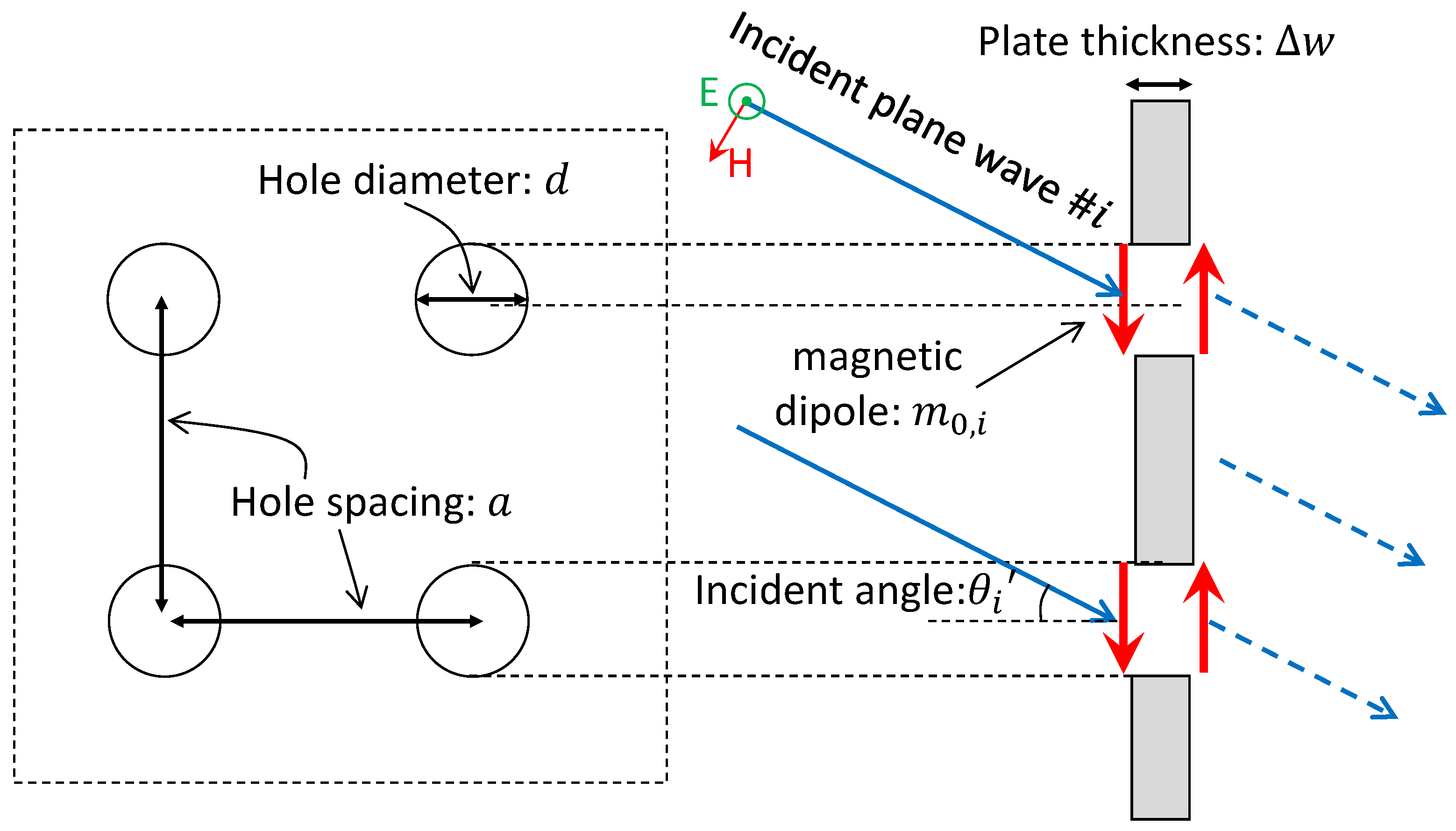
Figure 4.
Diagram of developed radio propagation measurement system.
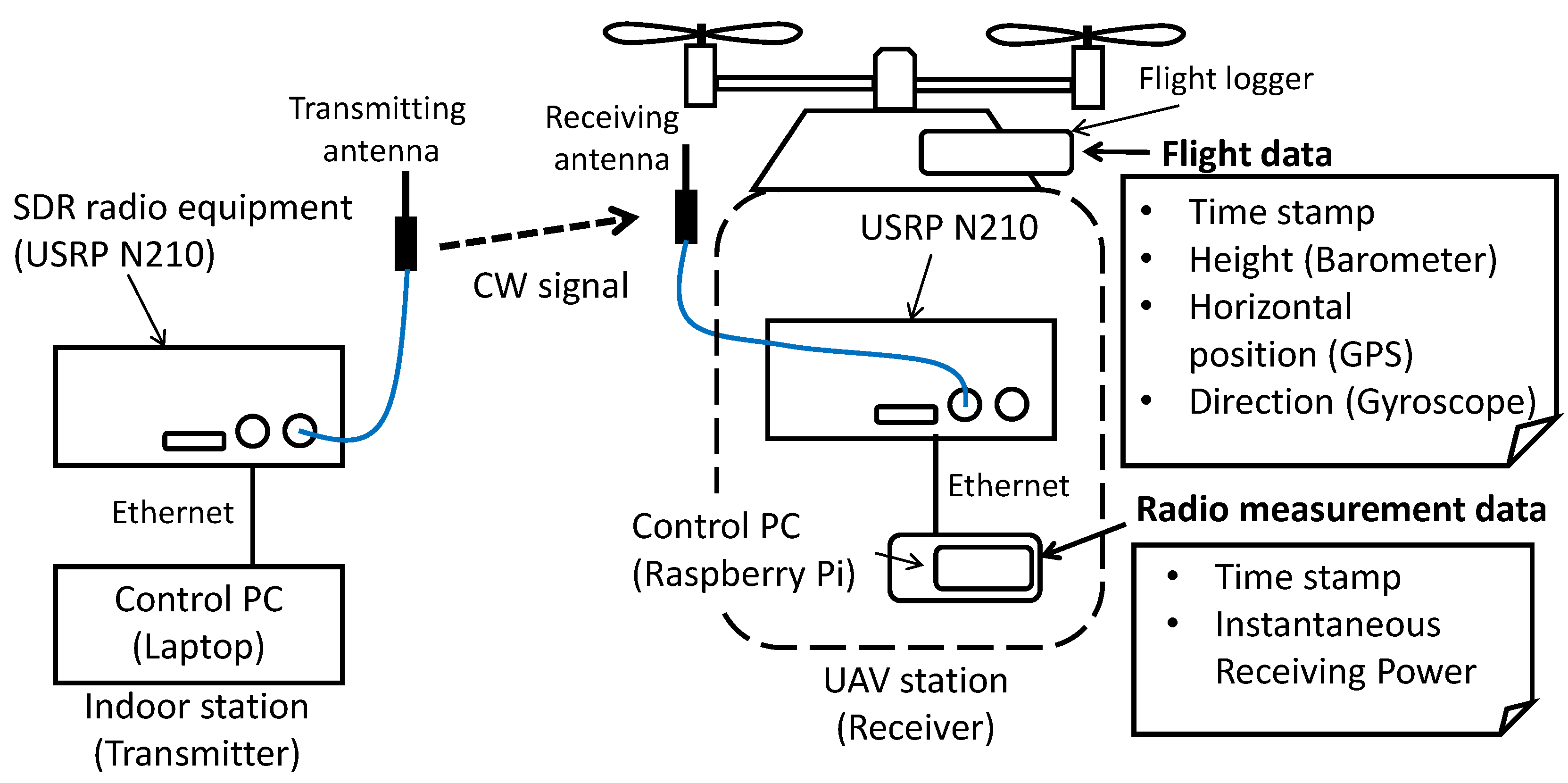
Figure 5.
Photo of the UAV station.
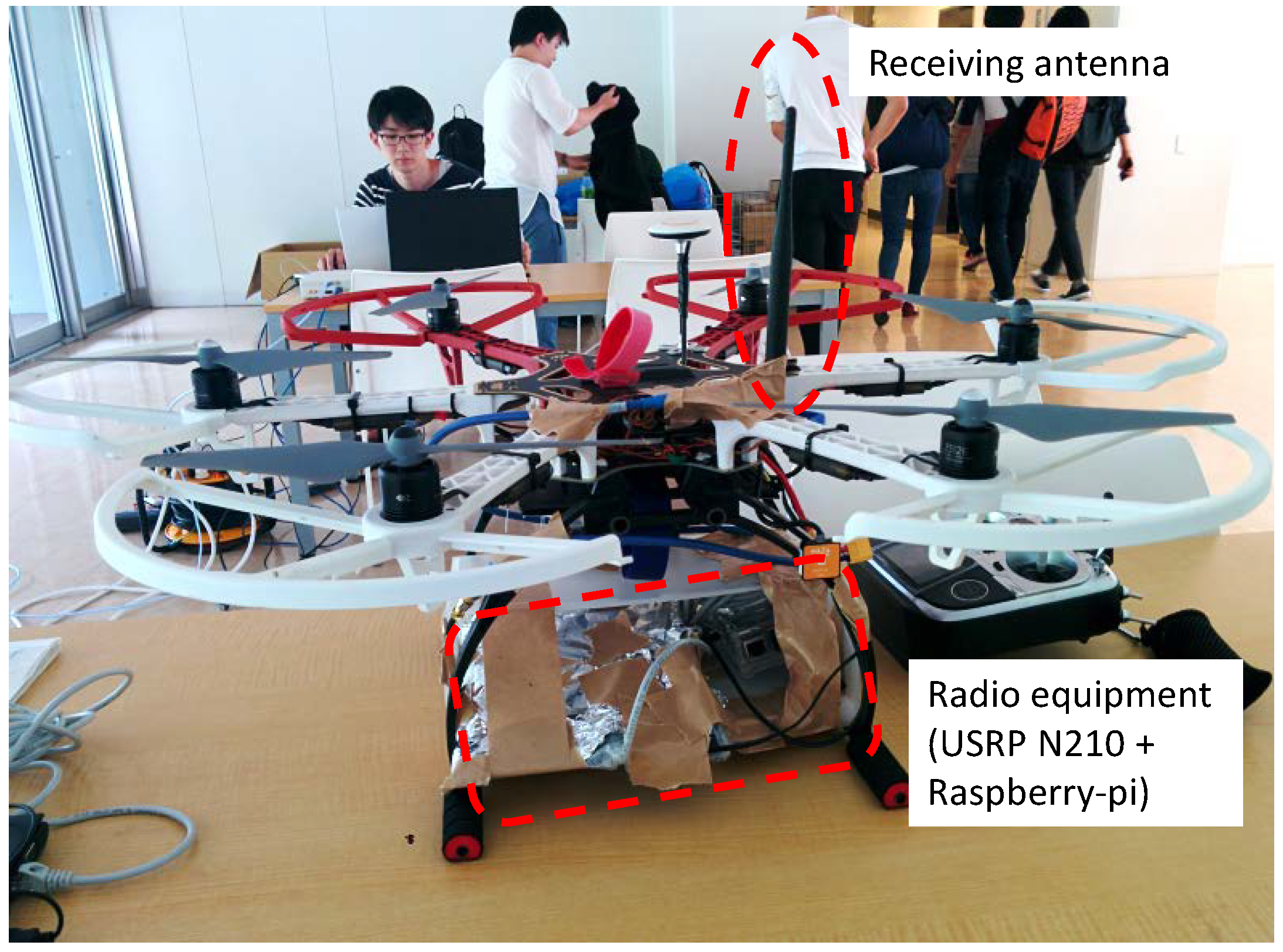
Figure 6.
Measurement overview ((a) measurement map, (b) outdoor view, (c) indoor view, and (d) window fence).
Figure 6.
Measurement overview ((a) measurement map, (b) outdoor view, (c) indoor view, and (d) window fence).

Figure 7.
3D environment model for the ray-tracing simulation ((a) outdoor view, (b) indoor view).
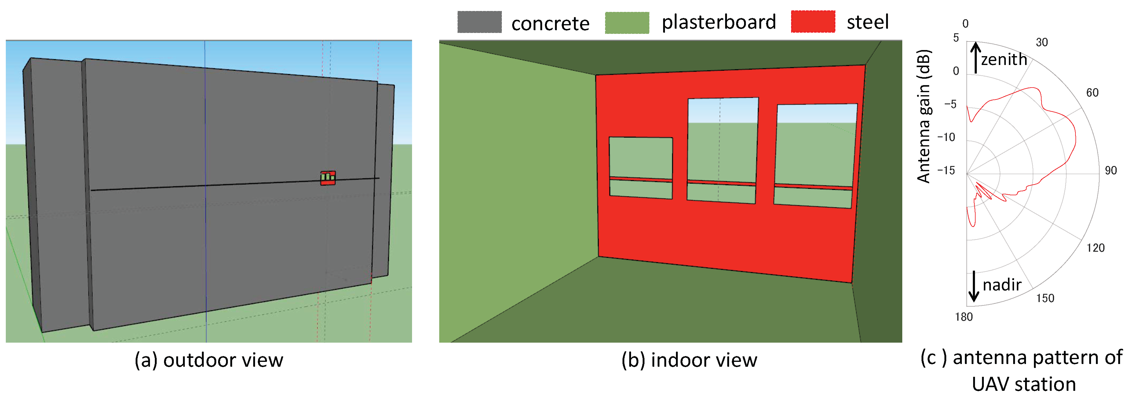
Figure 8.
The results of the MS1 setting ((a) receiving power profile (measurement), (b) receiving power profile (ray-tracing), (c) propagation route schema, (d) receiving power profile (ray-tracing, excluding diffraction rays), (e) receiving power profile (proposed method), and (f) prediction error (proposed method)).
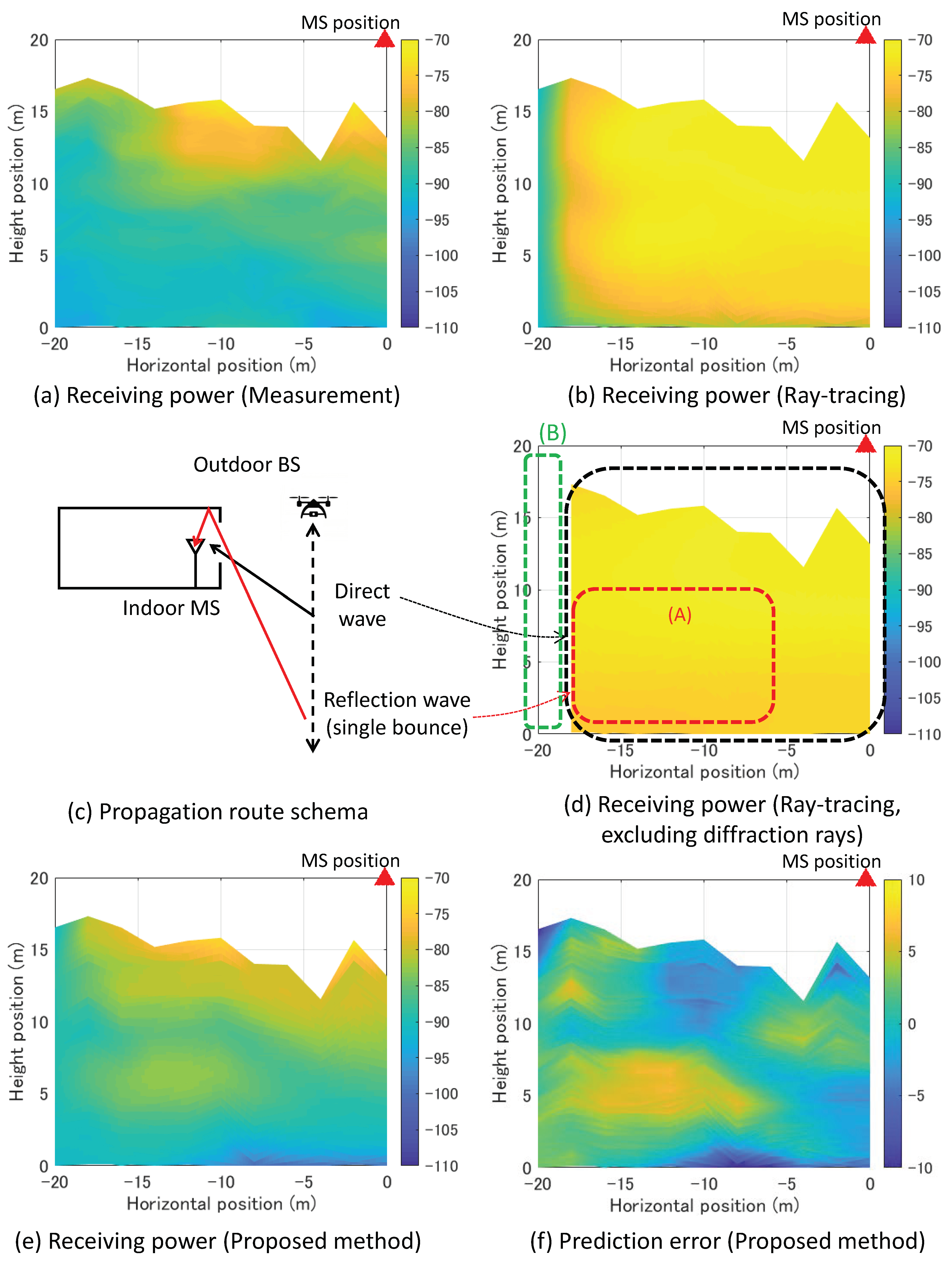
Figure 9.
The results of the MS3 setting ((a) receiving power profile (measurement), (b) receiving power profile (ray-tracing), (c) propagation route schema, (d) receiving power profile (ray-tracing, excluding diffraction rays), (e) receiving power profile (proposed method), and (f) prediction error (proposed method)).

Figure 10.
Prediction error CDF (error = simulation − measurement).

Table 1.
Measurement parameters.
| Radio Equipment | |
|---|---|
| Center frequency | 4.89 GHz |
| Transmit power | 11.5 dBm |
| Transmit signal | CW |
| Receiver dynamic range | From −120 dBm to −30 dBm |
| Tx/Rx antennas | Dipole (2.14 dBi) |
| Polarization | Vertical polarization |
| Antenna height (UAV) | From 0 m to 15 m |
| Indoor floor height | 20 m (building), 7 m (cafeteria) |
| Antenna height (indoor) | 1.7 m from floor |
| Receiver sampling rate | 100 Hz |
| Moving average | 2 m (horizontal) 1 m (vertical) |
| UAV equipment | |
| Flight controller | DJI NAZA-M v2 |
| Flight recorder | DJI iOSD MARK II |
| UAV sensor | 100 Hz |
| recording rate | |
Table 2.
Simulation parameters.
| Ray-Tracing Simulation | |
|---|---|
| Calculation Method | Method of Imaging |
| Number of reflections | 3 |
| Number of diffractions | 1 |
| Number of transmissions | 1 |
| Material parameters | Concrete: |
| (: relative permittivity | Ground: |
| : conductivity) | Metal: |
| Plaster board: | |
| Equivalent dielectric plate calculation | |
| Plate width | 3 mm |
| Hole diameter d | 20 mm |
| Hole spacing a | 30 mm |
Table 3.
Prediction error summary (error = simulation − measurement).
| Ray-Tracing | Proposed Method | |||||||
|---|---|---|---|---|---|---|---|---|
| MS1 | MS2 | MS3 | Total | MS1 | MS2 | MS3 | Total | |
| mean (dB) | 11.1 | 8.0 | 0.4 | 7.0 | 0.3 | 1.5 | −3.9 | −0.5 |
| standard deviation (dB) | 4.8 | 8.8 | 6.7 | 8.2 | 3.4 | 6.0 | 4.8 | 5.3 |
© 2019 by the authors. Licensee MDPI, Basel, Switzerland. This article is an open access article distributed under the terms and conditions of the Creative Commons Attribution (CC BY) license (http://creativecommons.org/licenses/by/4.0/).
Share and Cite
MDPI and ACS Style
Saito, K.; Fan, Q.; Keerativoranan, N.; Takada, J.-i. Site-Specific Propagation Loss Prediction in 4.9 GHz Band Outdoor-to-Indoor Scenario. Electronics 2019, 8, 1398. https://doi.org/10.3390/electronics8121398
AMA Style
Saito K, Fan Q, Keerativoranan N, Takada J-i. Site-Specific Propagation Loss Prediction in 4.9 GHz Band Outdoor-to-Indoor Scenario. Electronics. 2019; 8(12):1398. https://doi.org/10.3390/electronics8121398
Chicago/Turabian StyleSaito, Kentaro, Qiwei Fan, Nopphon Keerativoranan, and Jun-ichi Takada. 2019. "Site-Specific Propagation Loss Prediction in 4.9 GHz Band Outdoor-to-Indoor Scenario" Electronics 8, no. 12: 1398. https://doi.org/10.3390/electronics8121398
Note that from the first issue of 2016, this journal uses article numbers instead of page numbers. See further details here.