Abstract
Recently, model predictive control (MPC) is increasingly applied to path tracking of mobile devices, such as mobile robots. The characteristics of these MPC-based controllers are not identical due to the different approaches taken during design. According to the differences in the prediction models, we believe that the existing MPC-based path tracking controllers can be divided into four categories. We named them linear model predictive control (LMPC), linear error model predictive control (LEMPC), nonlinear model predictive control (NMPC), and nonlinear error model predictive control (NEMPC). Subsequently, we built these four controllers for the same mobile robot and compared them. By comparison, we got some conclusions. The real-time performance of LMPC and LEMPC is good, but they are less robust to reference paths and positioning errors. NMPC performs well when the reference velocity is high and the radius of the reference path is small. It is also robust to positioning errors. However, the real-time performance of NMPC is slightly worse. NEMPC has many disadvantages. Like LMPC and LEMPC, it performs poorly when the reference velocity is high and the radius of the reference path is small. Its real-time performance is also not good enough.
1. Introduction
Model predictive control (MPC) is an optimal control method that emerged in the 1970s. MPC usually has two key steps. Firstly, a prediction model should be built based on the mathematical model. This prediction model can predict all possible future states based on the current state and all feasible control inputs. Secondly, the state that is closest to the reference state in the possible future state is found by optimizing the objective function, and the control input corresponding to this state is obtained.
All of the methods that involve these two key steps can be called MPC. Recently, MPC is widely used in path tracking of mobile devices, such as unmanned vehicles, wheeled mobile robots, and drones. However, the design of these MPC-based path tracking controllers is not consistent. We can see that preliminary comparisons of these controllers have been reported in some papers. However, the comprehensive review and comparison have not been completed. Hence, we think that it is necessary to carry out this work.
In this paper, the classification principle of MPC is the mathematical logic of the prediction model, that is, the modeling idea. We classify MPC into linear MPC (LMPC), linear error MPC (LEMPC), nonlinear MPC (NMPC), and nonlinear error MPC (NEMPC), according to the nonlinear characteristics and output state quantities of the prediction model.
1.1. LMPC
The application of MPC to path tracking has a long history. If we only trace back to thirty years ago, the first related paper that can be retrieved is the work of Hess et al. []. They designed a path tracking controller for helicopters that are based on MPC. The feature of this controller is that the prediction model can work through matrix operations because the model of mobile devices is linearized.
In 1991, Ollero et al. designed a path tracking controller for mobile robots in a similar way, they proposed a linearized time discrete model for prediction []. In 2006, Keen et al. proposed a vehicle steering controller that is based on the linearized model []. Also in 2006, Lages et al. designed a controller for path tracking of mobile robots and named this method as linearized MPC []. In 2007, Falcone et al. also designed a steering controller for vehicles based on the linearized model and named this method as linear time-varying model predictive control (LTV-MPC) [,,].
Since then, more research results of path tracking based on this method have emerged [,,,,,,,,,,,,,,,,,,,,,]. In these studies, Meola et al. [] and Yakub et al. [] compared LTV-MPC and linear quadratic regulator (LQR) and showed that LTV-MPC performed better than LQR in terms of path tracking accuracy. Gong et al. [] introduced LTV-MPC-based path tracking to China first and promoted the development of this field in this country.
In [,,,,,,,,,,,,,,,,,,,,,,,,,,,,], although the devices being controlled are not identical, the control method used is the same. However, in these papers, the names of the control methods are not the same. Accordingly, we think that it is necessary to unify the naming. We believe that this control method can be simply named LMPC since no path tracking based on linear time-invariant model predictive control is found.
1.2. LEMPC
We have found another design approach that also enables prediction models to work through matrix operations. The key to this design approach is to convert kinematics models into error models according to geometric relationships and then linearizing error models.
Klančar et al. first proposed a LEMPC controller for path tracking of mobile robots []. They named this method tracking error MPC. Nayl et al. first used this method to design a path tracking controller for articulated vehicles [,,,]. They named this method switching MPC. In their work, the fact that this switching MPC outperforms LQR and feedback linearization in path tracking accuracy is proven. In 2017, Kang et al. designed a path tracking controller for front-wheel steering vehicles in a similar way []. Additionally, in 2017, Gutjahr et al. proposed a similar controller, but they named the control method LTV-MPC [].
The performance of the linearized MPC in [,,,,,,] is not exactly the same as in [,,,,,,,,,,,,,,,,,,,,,,,,,,,,] due to the different linearization process when compared to LMPC. To avoid confusion, we hope to harmonize the naming. In view of the common features of [,,,,,,], we think that it is better to call this control method linear error MPC (LEMPC).
1.3. NMPC
The most distinguishing feature of NMPC is that the nonlinear model of controlled mobile devices is directly discretized as the prediction model. Hence, the state variables of the NMPC are the pose states of the vehicles, and the errors between these states and the tracking target points in the prediction horizon are the penalty items. In other words, in the NMPC prediction model, future errors are related to all tracking target points in the prediction horizon. However, since this prediction model is nonlinear, it can only predict possible future state by iterating, not through matrix operations.
In 1994–1999, Gómez-Ortega et al. proposed the NMPC controller and improved the real-time performance of the controller by using artificial neural networks or genetic algorithms [,,,,]. After 2000, researchers have proposed more NMPC-based path tracking controllers [,,,,,,,,,,,,,,,,,,,]. In these studies, Künhe et al. [], Oyelere et al. [], and Li et al. [] have compared NMPC and LMPC. We [] have compared NMPC and LEMPC. The results of [,,,] show that the real-time performance of NMPC is poor, but the path tracking accuracy is high. In addition, Ghaemi et al. proposed a new optimization algorithm and claimed that it can help to improve the real-time performance of NMPC [].
The above evidence indicates that NMPC is a control method that is superior to LMPC and LEMPC, but we have found that another MPC method is also called NMPC. For the sake of distinction, we make a definition here. It is NMPC that the nonlinear model of mobile devices is directly used as the prediction model. It is the NEMPC that the model of the mobile device is transformed into a nonlinear error model by geometric relations.
1.4. NEMPC
In NEMPC, the state variable is the error, and its initial value is the error of the current pose of the vehicle and the first tracking target point in the prediction horizon. In other words, in the prediction model of NEMPC, future errors are not related to the target points other than the first tracking target point in the prediction horizon.
The paper that we can find, which was the earliest to adopt the nonlinear error model as the prediction model, is the work of Gu et al. []. This model might come from the path tracking of mobile robots based on feedback control []. When compared with the linear error model, the most important feature of the nonlinear error model is that nonlinear terms are not omitted. Hence, the prediction model that is based on the nonlinear error model also cannot work through the matrix operation.
In 2009, Kanjanawanishkul et al. designed a path tracking controller for mobile robots based on the nonlinear error model []. They call this control method NMPC. In 2014, Wang et al. proposed a path tracking controller for unmanned aerial vehicles that was based on a similar model []. They also call this control method NMPC. In some subsequent work, this control method is still called NMPC [,,,].
At present, we have not found other researchers who have noticed the difference between NEMPC and NMPC. The comparison between NEMPC and LMPC or LEMPC also has not been reported. Therefore, we believe that it is necessary to compare these control methods.
1.5. MPC and Intelligent Control
In recent years, the research results of the combination of MPC and intelligent control methods have increased. In the early research, Gómez-Ortega et al. used the neural network to learn NMPC offline [,,,] and accelerated the NMPC solution process by genetic algorithm []. Yang et al. [] and Gu et al. [] used neural networks as the prediction models. Recently, some MPC-based controllers using reinforcement learning to correct the parameters of prediction models have also been published [,,,].
There is no doubt that the above jobs are innovative and the combination of intelligent control and MPC is a very important trend. But these jobs are improvements based on LMPC or NMPC. The difference between LMPC and NMPC has not been taken seriously. In other words, the intelligent control method can be combined with NMPC or with LMPC, and we should find out which MPC is more suitable for being combined.
With the rapid integration of intelligent control and MPC, we have to face this problem. Accordingly, in this paper, we will compare LMPC, LEMPC, NMPC, and NEMPC. Since intelligent control does not completely change the difference between MPC-based controllers, we no longer consider MPC combined with intelligent control as the object of comparison.
1.6. Contribution of This Paper
In this paper, there are two contributions. First, we re-divided the MPC-based research results into four categories. The classification principle of MPC is the modeling idea of the prediction model. In the new classification, some confusion has been avoided. These confusions are listed below. In [,,,,,,,,,,,,,,,,,,,,,,,,,,,,], there are similar prediction models, but the name is not uniform. In [] and [], the prediction models are different, but they are all called LTV-MPC. There are two control methods in [,,,,,,,,,,,,,,,,,,,,,,,,,,,,,,,,], but they are all called NMPC. Second, we compared LMPC, LEMPC, NMPC, and NEMPC based on the same simulation conditions. The comparison consists of two parts. The first is the test of controllers at different velocities without positioning errors. Followed by the performance of controllers with different positioning errors.
The rest of this paper is arranged, as follows. Section 2 introduces the design of four controllers. In Section 3, the comparison of controllers at different velocities is presented. In Section 4, the comparison of controllers with different positioning errors is shown. Moreover, there is a brief conclusion in the last section.
2. Design of Controllers
In this paper, a classical kinematics model of mobile robots is adopted to ensure the generality. All of the controllers are based on the same model. Referring to our previous work [], the classic kinematics model is:
where is the coordinate of the mobile robot, is the heading angle, is the velocity, and is the heading angle speed.
We can rewrite (1) as a vector form:
where:
Referring to [], if the control period is 0.05 s, the constraints of the velocity and heading angle speed in each control period are:
2.1. LMPC Controller
First, linearize the (2) based on Jacobian linearization:
where:
represents the predicted state at the time , and represents the possible input at the time , represents the increment of the control input. When , these variables represent the actual values of the previous control cycle.
Assuming that the predicted horizon is and the control horizon is , the state in the predicted horizon is:
Rewrite (7) as a matrix operation formula:
where:
The prediction model of LMPC is (11).
Then we can design the optimization objective function to be:
where is the linearized state information of the tracking target point. This point is the point closest to the mobile robot on the reference path. and are weight matrices.
We can rewrite (16) as:
Since the linearized state information of the tracking target point is:
We can assume:
That is:
Because:
Assuming:
Then:
where:
Combined with the constraint (4), the LMPC controller is:
2.2. LEMPC Controller
The error between the mobile robot and the tracking target point can be converted to the coordinate system on mobile robots. The coordinate conversion process is described in our work []. (26) is the result of the conversion:
Subsequently, linearizing (26):
where:
Assuming that the predicted horizon is and the control horizon is , the state in the predicted horizon is:
Rewrite (7) as a matrix operation formula:
where:
The prediction model of LEMPC is (33).
Then we can design the optimization objective function to be:
That is:
Then:
where:
Combined with the constraint (4), the LEMPC controller is:
2.3. NMPC Controller
In the NMPC controller, the discretized mobile robot model is directly used as the prediction model.
Discretize (2):
That is:
Assuming that the predicted horizon is and the control horizon is , the state in the predicted horizon is:
Afterwards, we can define the error between the predicted state and the reference path in the predicted horizon:
where:
The information for tracking the first target point is in (48). This point is the closest point on the reference path to the mobile robot.
We need to determine other tracking target points according to the reference path and the first tracking target point since it is necessary to input tracking target points to the NMPC controller. The arc length of the reference path between each tracking target point is equal to , where is the reference velocity of the mobile robot.
The control input increment is:
Combining (46) and (48), the objective function of the rolling optimization can be designed as:
Subsequently, the NMPC controller is:
2.4. NEMPC Controller
The error between the mobile robot and the tracking target point can be converted to the coordinate system on mobile robots:
Assuming the state of tracking target point:
Subsequently, we can get the following formula by deriving (51):
Substituting (1) and simplifying it:
Abstract (54) as:
where:
Discretize (56):
Assuming that the predicted horizon is Np and the control horizon is Nc, the state in the predicted horizon is:
Subsequently, the objective function can be designed as:
Afterwards, the NEMPC controller is:
3. Comparison at Different Velocities
MATLAB/Simulink R2018b compares the controllers. The computer for simulation is equipped with the Intel(R) Core(TM) i5-8500 CPU @ 3.00 GHz, RAM 8.00 GB, Windows 10 Pro. To test the real-time, we enabled Real-Time Synchronization. In solving (25), (42), (50), and (60), active-set is employed, and the default accuracy of active-set is 10−6. Each controller controls the same model. The parameters of controllers are shown in Table 1. Where is the unit matrix. The reference path consists of the straight line and the arc. The radius of the arc is 2.5 m. The displacement error and heading error are the targets of comparison. Their definitions are shown in [].

Table 1.
Parameters in all controllers.
3.1. Velocity Is 2 m/s
The simulation results at the reference velocity of 2 m/s are shown in Figure 1, Figure 2, Figure 3, Figure 4, Figure 5 and Figure 6. In this case, all of the controllers can control the mobile robot tracking reference path. At 2 m/s, the displacement error and the heading error of controllers are small. The real-time performance of NMPC and NEMPC is worse than that of LMPC and LEMPC. However, all controllers have much less computation time in the control period than the control period. Table 2 shows the maximum absolute values.
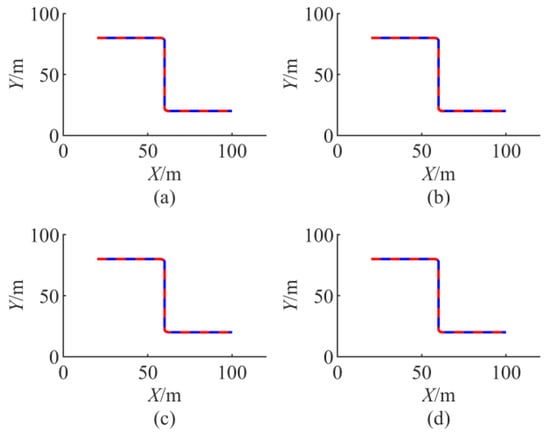
Figure 1.
The trajectory when velocity is 2 m/s. The red line is the trajectory. The blue line is the reference path. (a) linear model predictive control (LMPC). (b) linear error model predictive control (LEMPC). (c) nonlinear model predictive control (NMPC). (d) nonlinear error model predictive control (NEMPC).
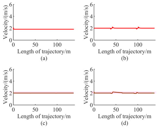
Figure 2.
The velocity when velocity is 2 m/s. (a) LMPC. (b) LEMPC. (c) NMPC. (d) NEMPC.
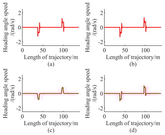
Figure 3.
The heading angle speed when velocity is 2 m/s. (a) LMPC. (b) LEMPC. (c) NMPC. (d) NEMPC.
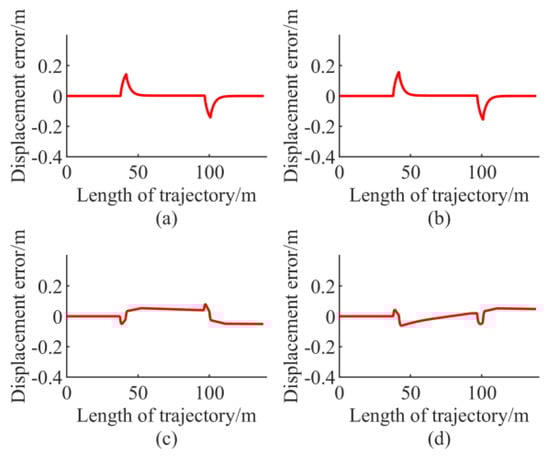
Figure 4.
The displacement error when velocity is 2 m/s. (a) LMPC. (b) LEMPC. (c) NMPC. (d) NEMPC.
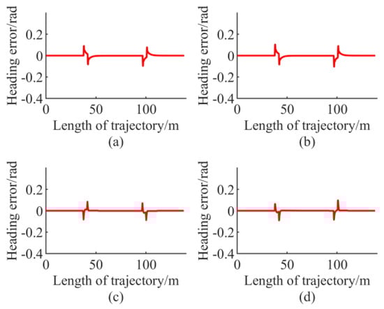
Figure 5.
The heading error when velocity is 2 m/s. (a) LMPC. (b) LEMPC. (c) NMPC. (d) NEMPC.
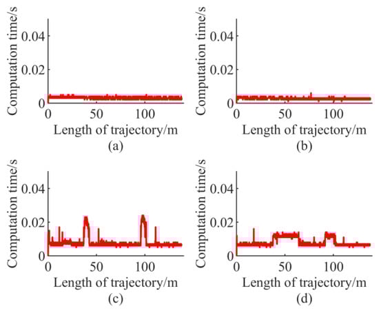
Figure 6.
The computation time when velocity is 2 m/s. (a) LMPC. (b) LEMPC. (c) NMPC. (d) NEMPC.
Table 2.
The maximum absolute values when velocity is 2 m/s.
3.2. Velocity Is 3 m/s
When the reference speed is 3 m/s, the simulation results are shown in Figure 7, Figure 8, Figure 9, Figure 10, Figure 11 and Figure 12. LMPC, NMPC, and NEMPC still can control the mobile robot tracking reference path. The error of LEMPC is divergent. Since it is meaningless to continue the simulation after the error diverges, we define that: Control failure when the absolute value of the heading error is greater than 1.5 rad. The simulation will be stopped halfway if the absolute value of heading error is greater than 1.5 rad.
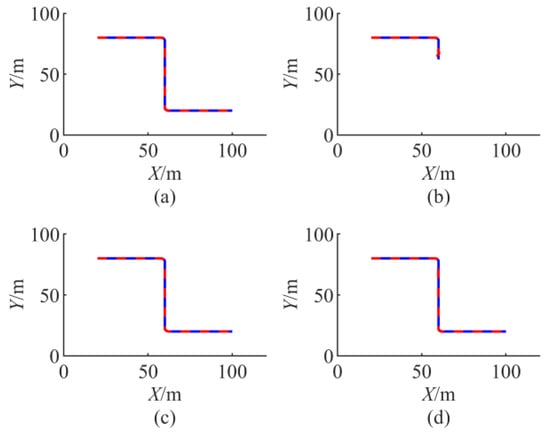
Figure 7.
The trajectory when velocity is 3 m/s. The red line is the trajectory. The blue line is the reference path. (a) LMPC. (b) LEMPC. (c) NMPC. (d) NEMPC. The blue line is the reference path.
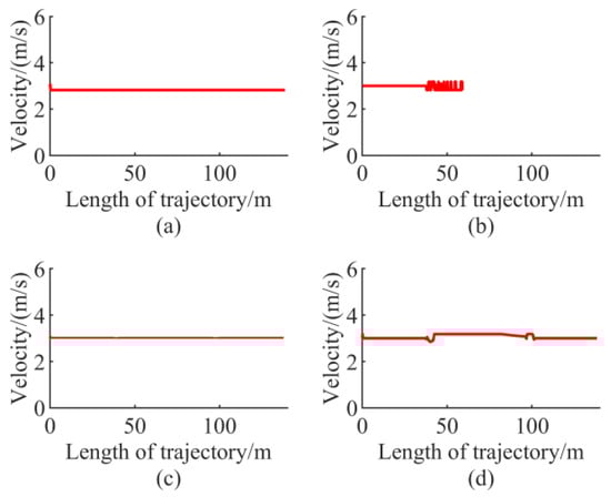
Figure 8.
The velocity when velocity is 3 m/s. (a) LMPC. (b) LEMPC. (c) NMPC. (d) NEMPC.
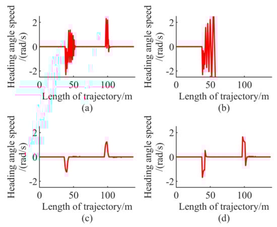
Figure 9.
The heading angle speed when velocity is 3 m/s. (a) LMPC. (b) LEMPC. (c) NMPC. (d) NEMPC.
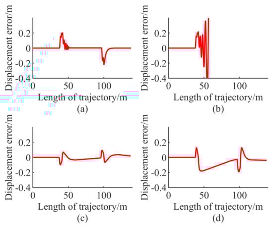
Figure 10.
The displacement error when velocity is 3 m/s. (a) LMPC. (b) LEMPC. (c) NMPC. (d) NEMPC.
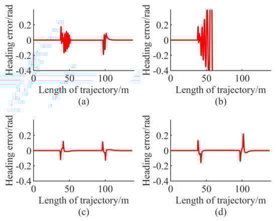
Figure 11.
The heading error when velocity is 3 m/s. (a) LMPC. (b) LEMPC. (c) NMPC. (d) NEMPC.
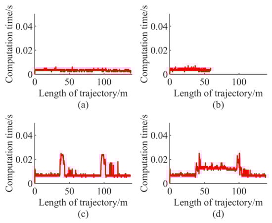
Figure 12.
The computation time when velocity is 3 m/s. (a) LMPC. (b) LEMPC. (c) NMPC. (d) NEMPC.
The maximum absolute values are shown in Table 3. The error of all MPC-based controllers increases with respect to that when the reference velocity is 2 m/s.
Table 3.
The maximum absolute values when velocity is 3 m/s.
The control inputs of the NMPC are the smoothest.
The real-time performance of NMPC and NEMPC is not as good as that of LMPC and LEMPC. However, the maximum computation time for all controllers is less than 0.05 s.
3.3. Velocity Is 4 m/s
Figure 13, Figure 14, Figure 15, Figure 16, Figure 17 and Figure 18 show the simulation results at the reference velocity of 4 m/s. NMPC and NEMPC still can control the mobile robot tracking reference path. The error of LMPC and LEMPC is divergent, and we stopped these two controllers halfway. The error of all MPC-based controllers increases with respect to that when the reference velocity is 3 m/s. Table 4 shows the maximum absolute values.
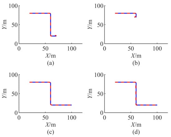
Figure 13.
The trajectory when velocity is 4 m/s. The red line is the trajectory. The blue line is the reference path. (a) LMPC. (b) LEMPC. (c) NMPC. (d) NEMPC.
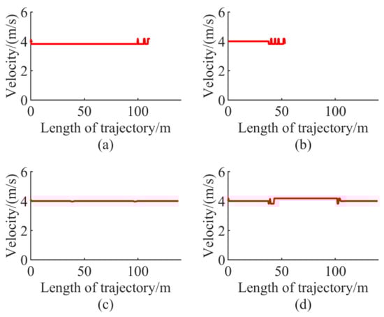
Figure 14.
The velocity when velocity is 4 m/s. (a) LMPC. (b) LEMPC. (c) NMPC. (d) NEMPC.
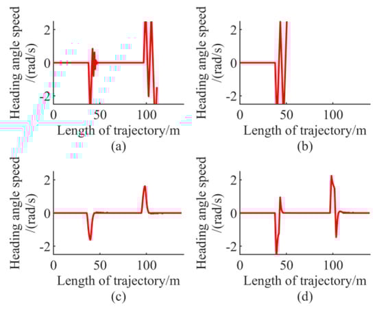
Figure 15.
The heading angle speed when velocity is 4 m/s. (a) LMPC. (b) LEMPC. (c) NMPC. (d) NEMPC.
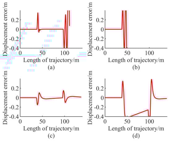
Figure 16.
The displacement error when velocity is 4 m/s. (a) LMPC. (b) LEMPC. (c) NMPC. (d) NEMPC.
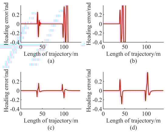
Figure 17.
The heading error when velocity is 4 m/s. (a) LMPC. (b) LEMPC. (c) NMPC. (d) NEMPC.
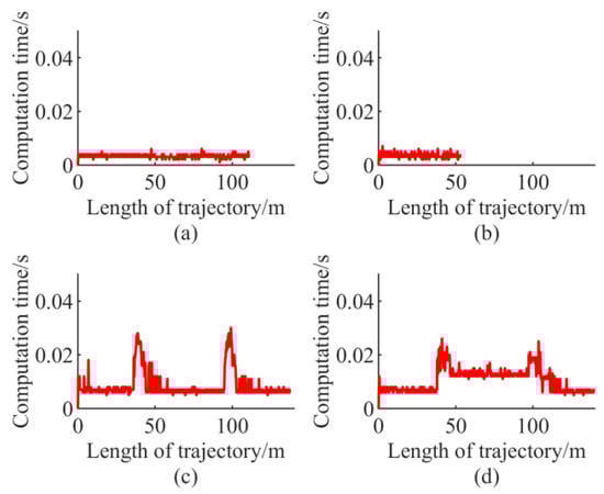
Figure 18.
The computation time when velocity is 4 m/s. (a) LMPC. (b) LEMPC. (c) NMPC. (d) NEMPC.
Table 4.
The maximum absolute values when velocity is 4 m/s.
Through three sets of comparisons, we can draw some obvious conclusions. First, the control input of NMPC is the smoothest. Second, LMPC and LEMPC have better real-time performance. Third, the maximum computation time of NMPC and NEMPC is also smaller than the control period. The real-time performance of these two MPC-based controllers is sufficient for the path tracking of mobile robots.
Figure 19 and Figure 20 show the trend of maximum absolute errors. From these two pictures, we can believe that, when using the weight matrix shown in Table 1, the stability of LMPC and LEMPC is poor and the ability of NEMPC to reduce residual error is not good enough. However, we have reason to doubt whether using different weight factors will lead to different results. Thus, we think more comparisons are needed.
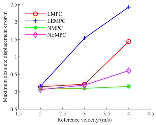
Figure 19.
The trend of the maximum absolute displacement error.
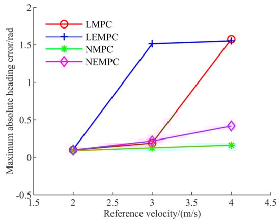
Figure 20.
The trend of the maximum absolute heading error.
3.4. Parameters Changed
For weight factors, we have studied in []. We have found that, when the weight of the heading error is increased in the objective function, the stability of the controller is increased, and, on the contrary, the ability of the controller to reduce the residual error is increased. Based on this experience, we present a new set of comparisons. Table 5 shows the new weight matrix.
Table 5.
Changed parameters in controllers.
The results of this set of the simulation are shown in Figure 21, Figure 22, Figure 23, Figure 24, Figure 25 and Figure 26. Table 6 shows the maximum absolute values. All of the controllers can control the mobile robot tracking reference path. As can be seen from Figure 24, increasing the weight of the heading error does improve the stability of the LMPC and LEMPC, but the maximum absolute error is still large. However, if the weight of the heading error is further increased, it is possible to cause a larger residual displacement error. Increasing the weight of the displacement error can improve the ability of NEMPC to reduce the residual error, but its maximum absolute error also is large. Adjusting the weight factor has little effect on the maximum error of NEMPC. Therefore, in this set of simulations, the maximum error of LMPC, LEMPC, and NEMPC is close to its minimum. Based on these results, we can see that adjusting the weighting factor does not reduce the errors that are produced by LMPC, LEMPC, and NEMPC during sharp turns. We discussed the trigger for this phenomenon in []. LMPC, LEMPC, and NEMPC predict future errors based on current errors, resulting in the inability to take the changing of the reference path into account. This is an important reason for the poor performance of these controllers.
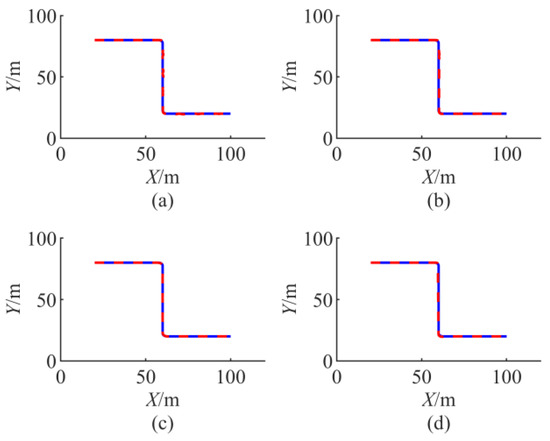
Figure 21.
The trajectory when parameters changed. The red line is the trajectory. The blue line is the reference path. (a) LMPC. (b) LEMPC. (c) NMPC. (d) NEMPC.
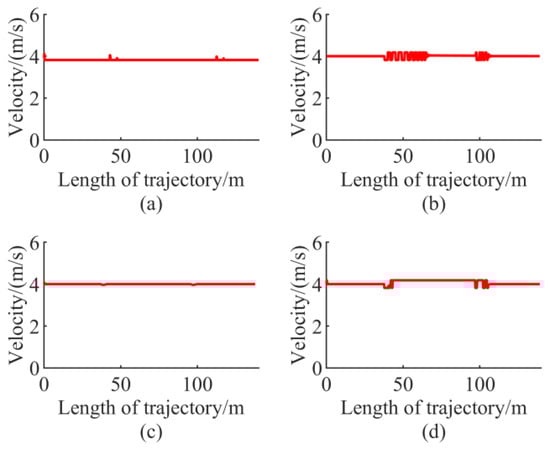
Figure 22.
The velocity when parameters changed. (a) LMPC. (b) LEMPC. (c) NMPC. (d) NEMPC.
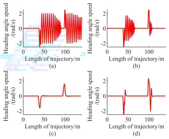
Figure 23.
The heading angle speed when parameters changed. (a) LMPC. (b) LEMPC. (c) NMPC. (d) NEMPC.
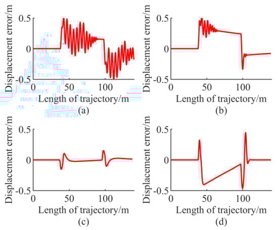
Figure 24.
The displacement error when parameters changed. (a) LMPC. (b) LEMPC. (c) NMPC. (d) NEMPC.
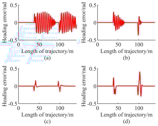
Figure 25.
The heading error when parameters changed. (a) LMPC. (b) LEMPC. (c) NMPC. (d) NEMPC.
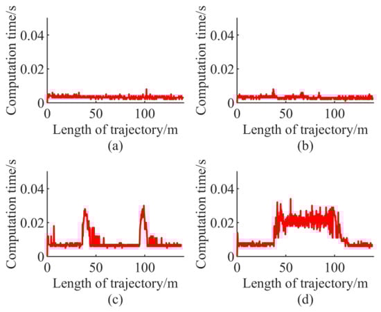
Figure 26.
The computation time when parameters changed. (a) LMPC. (b) LEMPC. (c) NMPC. (d) NEMPC.
Table 6.
The maximum absolute values after weight changing.
Therefore, we can draw conclusions on the accuracy of path tracking. When the reference velocity is low and the minimum radius of the reference path is large, the errors of LMPC, LEMPC, NMPC, and NEMPC are small. However, when the reference velocity is high or the minimum radius of the reference path is small, the performance of NMPC is better than that of other MPC methods.
4. Comparison with Different Positioning Errors
In the comparison of Section 3, errors of the positioning system are ignored. Therefore, we intend to compare the performance of these control methods with the impact of positioning error in this part. In the following two sets of simulations, we still use the parameters in Table 1. The reference velocity is 2 m/s.
4.1. Positioning Error in ±0.1 m
In the first set of simulations, we added white noise in the range of (−0.1 m, 0.1 m) in the and directions as the positioning errors. The simulation results with the positioning error in the range of (−0.1 m, 0.1 m) are shown in Figure 27, Figure 28, Figure 29, Figure 30, Figure 31 and Figure 32. In this case, all of the MPC-based controllers can control the mobile robot tracking reference path. From Figure 28 and Figure 29, we can see that control inputs of NMPC are smoother than those of other MPC-based methods. Table 7 shows the maximum absolute values of errors. The real-time performance of LMPC and LEMPC is still very good. The maximum calculation time of NMPC and NEMPC is also less than the control period.
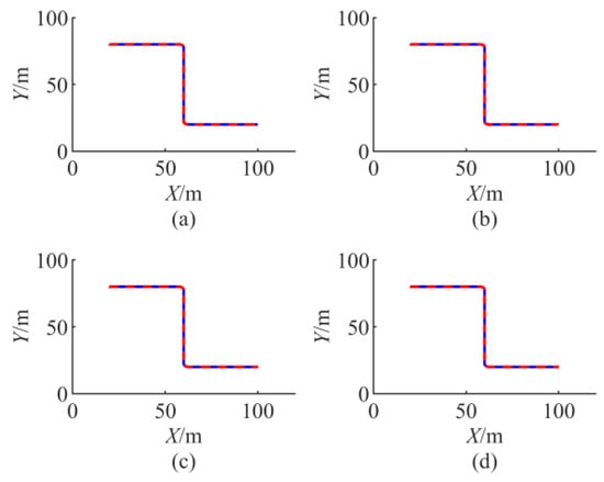
Figure 27.
The trajectory with the positioning error in ±0.1 m. The red line is the trajectory. The blue line is the reference path. (a) LMPC. (b) LEMPC. (c) NMPC. (d) NEMPC.
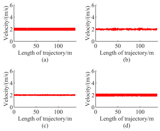
Figure 28.
The velocity with the positioning error in ±0.1 m. (a) LMPC. (b) LEMPC. (c) NMPC. (d) NEMPC.
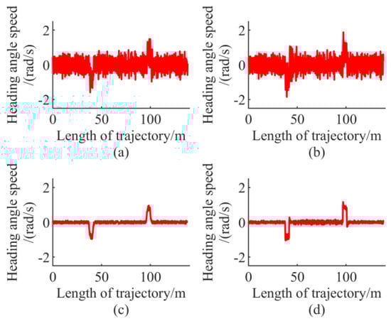
Figure 29.
The heading angle speed with the positioning error in ±0.1 m. (a) LMPC. (b) LEMPC. (c) NMPC. (d) NEMPC.
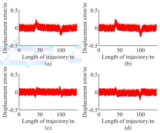
Figure 30.
The displacement error with the positioning error in ±0.1 m. (a) LMPC. (b) LEMPC. (c) NMPC. (d) NEMPC.
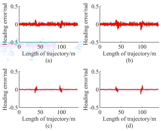
Figure 31.
The heading error with the positioning error in ±0.1 m. (a) LMPC. (b) LEMPC. (c) NMPC. (d) NEMPC.
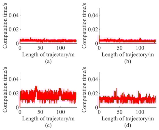
Figure 32.
The computation time with the positioning error in ±0.1 m. (a) LMPC. (b) LEMPC. (c) NMPC. (d) NEMPC.
Table 7.
The maximum absolute values with the positioning error in ±0.1 m.
4.2. Positioning Error in ±0.2 m
In the second set of simulations, we increased the positioning error to (−0.2 m, 0.2 m). Figure 33, Figure 34, Figure 35, Figure 36, Figure 37 and Figure 38 shows the simulation results. Control inputs of the NMPC are still the smoothest. The errors of LMPC and LEMPC are divergent. The maximum absolute values of errors are shown in Table 8. Real-time performance is still the same as the previous groups. The maximum calculation time of controllers is also less than the control period.
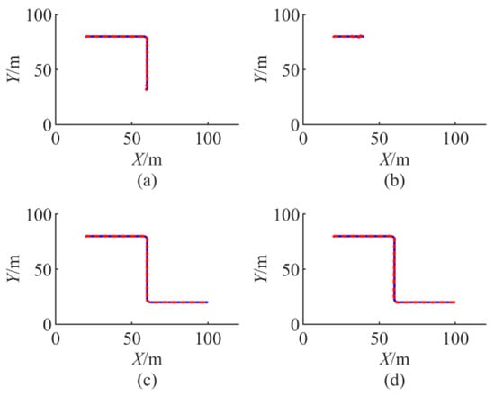
Figure 33.
The trajectory with the positioning error in ±0.2 m. The red line is the trajectory. The blue line is the reference path. (a) LMPC. (b) LEMPC. (c) NMPC. (d) NEMPC.
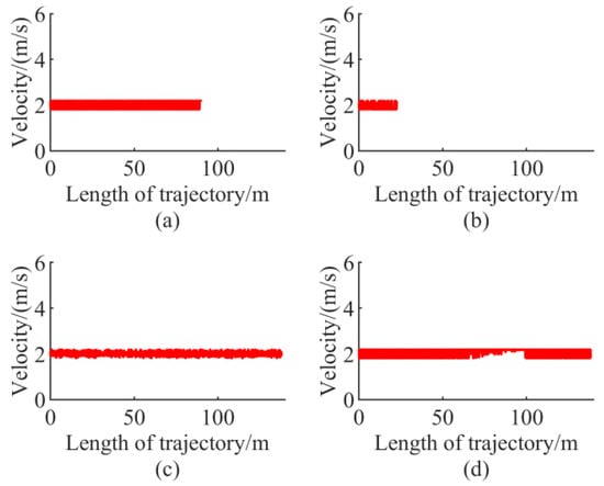
Figure 34.
The velocity with the positioning error in ±0.2 m. (a) LMPC. (b) LEMPC. (c) NMPC. (d) NEMPC.
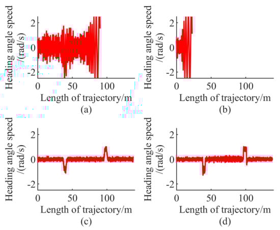
Figure 35.
The heading angle speed with the positioning error in ±0.2 m. (a) LMPC. (b) LEMPC. (c) NMPC. (d) NEMPC.
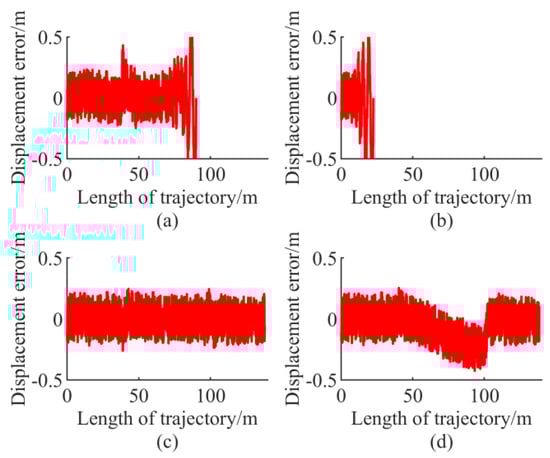
Figure 36.
The displacement error with the positioning error in ±0.2 m. (a) LMPC. (b) LEMPC. (c) NMPC. (d) NEMPC.
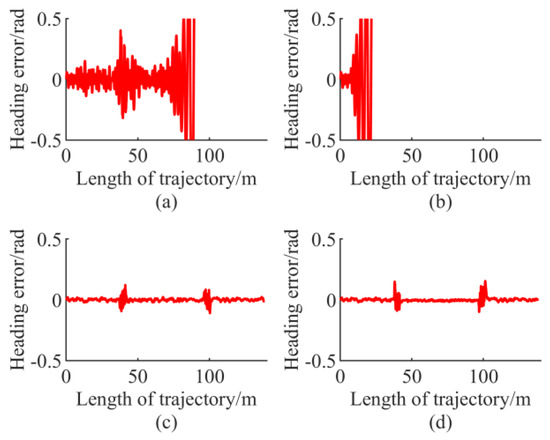
Figure 37.
The heading error with the positioning error in ±0.2 m. (a) LMPC. (b) LEMPC. (c) NMPC. (d) NEMPC.
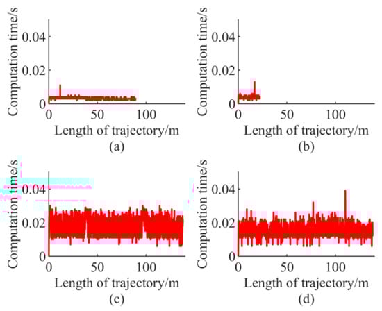
Figure 38.
The computation time with the positioning error in ±0.2 m. (a) LMPC. (b) LEMPC. (c) NMPC. (d) NEMPC.
Table 8.
The maximum absolute values with the positioning error in ±0.2 m.
4.3. Parameters Changed
To avoid instability, we adjusted the weighting factor again and gave the final set of comparisons. Table 9 shows the new weight coefficients. The positioning error is set in (−0.2 m, 0.2 m). Figure 39, Figure 40, Figure 41, Figure 42, Figure 43 and Figure 44 show the simulation results. The maximum absolute values of errors are shown in Table 10. After adjusting the weights, all of the controllers can control the mobile robot to complete the path tracking. However, the ability of LMPC and LEMPC to reduce residual errors is greatly diminished. The maximum absolute error of these two controllers is large. The maximum absolute values of errors are shown in Table 9. From these data, LMPC and LEMPC are less robust to positioning errors, but NMPC and NEMPC are robust to positioning errors.
Table 9.
Changed parameters in controllers.
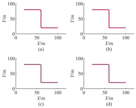
Figure 39.
The trajectory of the final set of comparison. The red line is the trajectory. The blue line is the reference path. (a) LMPC. (b) LEMPC. (c) NMPC. (d) NEMPC.
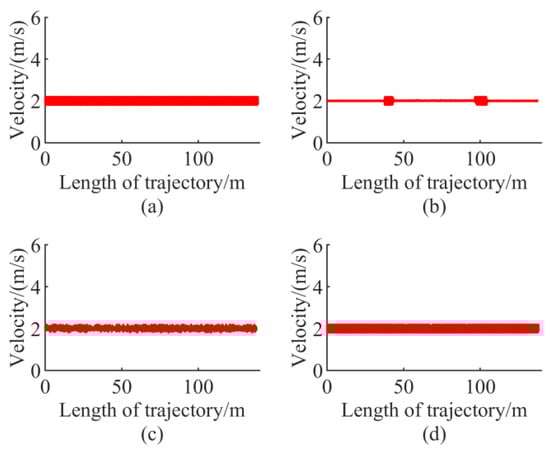
Figure 40.
The velocity of the final set of comparison. (a) LMPC. (b) LEMPC. (c) NMPC. (d) NEMPC.
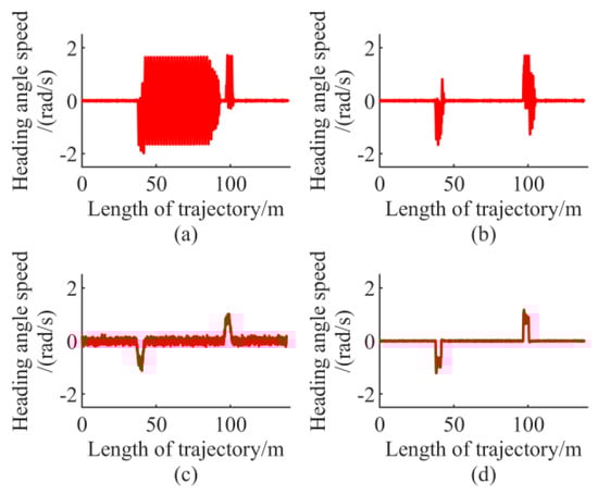
Figure 41.
The heading angle speed of the final set of comparison. (a) LMPC. (b) LEMPC. (c) NMPC. (d) NEMPC.
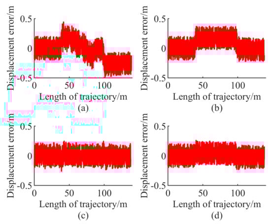
Figure 42.
The displacement error of the final set of comparison. (a) LMPC. (b) LEMPC. (c) NMPC. (d) NEMPC.
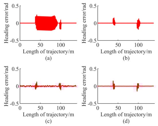
Figure 43.
The heading error of the final set of comparison. (a) LMPC. (b) LEMPC. (c) NMPC. (d) NEMPC.
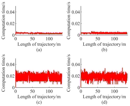
Figure 44.
The computation time of the final set of comparison. (a) LMPC. (b) LEMPC. (c) NMPC. (d) NEMPC.
Table 10.
The maximum absolute values after weight changing, with the positioning error in ±0.2 m.
5. Conclusions
In this paper, we reviewed the path tracking control method that is based on MPC. We found that the existing MPC-based path tracking control methods can be divided into four types according to the mathematical logic of the prediction model. Afterwards, we compared LMPC, LEMPC, NMPC, and NEMPC. Based on these comparison results and the results in papers, such as [,,,], we believe that the following conclusions and outlooks can be drawn.
First, the performance of LMPC and LEMPC is similar. The most significant advantage of these two control methods is good real-time performance. Their biggest drawback is that the error is large when the reference velocity is high and the radius of the reference path is small. Moreover, they are less robust to positioning errors. Thus, LMPC and LEMPC are suitable for low-cost scenarios where real-time requirements are high, but the operation velocity is slow and accuracy requirements are low. Advanced path planning and velocity planning can make the path tracking control system avoid the case that the reference speed is high and the radius of the reference path is small, which will help to improve the performance of the two control methods. Therefore, combining path planning, speed planning, and these two MPC control methods is a feasible way to improve the performance of path tracking, such as our work [].
Second, NMPC performs well when the reference velocity is high and the radius of the reference path is small. NMPC is robust to positioning errors. Moreover, the control input of the NMPC is the smoothest with or without positioning error. The most significant drawback of NMPC is its poor real-time performance. In this paper, the maximum calculation time of NMPC is less than the control period. However, when the model is more complicated, the real-time performance of NMPC may not be guaranteed. Thus, NMPC can be used in high-cost scenarios where the accuracy requirements are high and the computer hardware is advanced. Improving real-time performance is the most important issue in NMPC-based path tracking research.
Third, we found that NEMPC has no great advantages over other MPC methods. Its real-time performance is poor than that of LMPC and LEMPC. NEMPC also performs poorly when the reference velocity is high and the radius of the reference path is small. For robustness, it also has not greatly outperformed NMPC.
For MPC-based path tracking, there are still some issues that are not addressed in this paper. We will continue to study in the future, and we hope that more experts will work to solve these problems. Two notable problems are listed below. The similarities and differences of the proof of the stability of path tracking that is based on different MPC methods. Comparison of path tracking based on different MPC methods when the dynamic model of mobile devices is more complex.
Author Contributions
Conceptualization, G.B., Q.G., and Y.M.; methodology, G.B. and Q.G.; software, G.B. and L.L. (qianli12101993@163.com); validation, G.B. and L.L. (qianli12101993@163.com); investigation, G.B.; writing—original draft preparation, G.B.; writing—review and editing, Y.M., L.L. (liliu@ustb.edu.cn), W.L., and Q.G.; supervision, L.L. (liliu@ustb.edu.cn) and W.L.; project administration, L.L. (liliu@ustb.edu.cn) and W.L.; funding acquisition, L.L. (liliu@ustb.edu.cn), W.L., Y.M., and Q.G.
Funding
This research was funded by the National Key Research and Development Program of China, grant number 2018YFC0604403 and 2016YFC0802905, the National High Technology Research and Development Program of China (863 program), grant number 2011AA060408 and the Fundamental Research Funds for the Central Universities, grant number FRF-TP-17-010A2.
Conflicts of Interest
The authors declare no conflict of interest. The funders had no role in the design of the study; in the collection, analyses, or interpretation of data; in the writing of the manuscript, or in the decision to publish the results.
References
- Hess, R.A.; Jung, Y.C. An application of generalized predictive control to rotorcraft terrain-following flight. IEEE Trans. Syst. Man Cybern. 1989, 19, 955–962. [Google Scholar] [CrossRef]
- Ollero, A.; Amidi, O. Predictive path tracking of mobile robots. Application to the CMU Navlab. In Proceedings of the Fifth International Conference on Advanced Robotics, Robots in Unstructured Environments, Pisa, Italy, 19–22 June 1991. [Google Scholar]
- Keen, S.D.; Cole, D.J. Steering control using model predictive control and multiple internal models. AVEC 2006, 2006, 599–604. [Google Scholar]
- Lages, W.F.; Alves, J.A.V. Real-time control of a mobile robot using linearized model predictive control. IFAC Proc. Vol. 2006, 39, 968–973. [Google Scholar] [CrossRef]
- Falcone, P.; Borrelli, F.; Asgari, J.; Tseng, H.E.; Hrovat, D. Predictive active steering control for autonomous vehicle systems. IEEE Trans. Control Syst. Technol. 2007, 15, 566–580. [Google Scholar] [CrossRef]
- Falcone, P.; Tseng, H.E.; Asgari, J.; Borrelli, F.; Hrovat, D. Integrated braking and steering model predictive control approach in autonomous vehicles. IFAC Proc. Vol. 2007, 40, 273–278. [Google Scholar] [CrossRef]
- Falcone, P.; Tufo, M.; Borrelli, F.; Asgari, J.; Tseng, H.E. A linear time varying model predictive control approach to the integrated vehicle dynamics control problem in autonomous systems. In Proceedings of the 2007 46th IEEE Conference on Decision and Control, New Orleans, LA, USA, 12–14 December 2007; pp. 2980–2985. [Google Scholar] [CrossRef]
- Raffo, G.V.; Gomes, G.K.; Normey-Rico, J.E.; Kelber, C.R.; Becker, L.B. A predictive controller for autonomous vehicle path tracking. IEEE Trans. Intell. Transp. 2009, 10, 92–102. [Google Scholar] [CrossRef]
- Katriniok, A.; Abel, D. LTV-MPC approach for lateral vehicle guidance by front steering at the limits of vehicle dynamics. In Proceedings of the CDC and ECC, Orlando, FL, USA, 12–15 December 2011; pp. 6828–6833. [Google Scholar]
- Barbarisi, O.; Palmieri, G.; Scala, S.; Glielmo, L. LTV-MPC for yaw rate control and side slip control with dynamically constrained differential braking. Eur. J. Control 2009, 15, 468–479. [Google Scholar] [CrossRef]
- Palmieri, G.; Barbarisi, O.; Scala, S.; Glielmo, L. A preliminary study to integrate LTV-MPC lateral vehicle dynamics control with a slip control. In Proceedings of the CDC Held Jointly with CCC, Shanghai, China, 15–18 December 2009; pp. 4625–4630. [Google Scholar]
- Meola, D.; Gambino, G.; Palmieri, G.; Glielmo, L. A comparison between LTV-MPC and LQR yaw rate-side slip controller. IFAC Proc. Vol. 2009, 42, 154–159. [Google Scholar] [CrossRef]
- Gong, J.W.; Jiang, Y.; Xu, W. Chapter 3 Model Predictive Control Algorithm Fundamentals and Simulation Analysis. In Model Predictive Control for Self-Driving Vehicles; Beijing Institute of Technology Press: Beijing, China, 2014; pp. 36–73. (In Chinese) [Google Scholar]
- Lima, P.F.; Trincavelli, M.; Mårtensson, J.; Wahlberg, B. Clothoid-based model predictive control for autonomous driving. In Proceedings of the ECC, Linz, Austria, 15–17 July 2015. [Google Scholar]
- Yakub, F.; Mori, Y. Comparative study of autonomous path-following vehicle control via model predictive control and linear quadratic control. Proc. Inst. Mech. Eng. Part D J. Autom. Eng. 2015, 229, 1695–1714. [Google Scholar] [CrossRef]
- Gong, J.W.; Xu, W.; Jiang, Y.; Liu, K.; Guo, H.F.; Sun, Y.J. Multi-constrained model predictive control for autonomous ground vehicle trajectory tracking. J. Beijing Inst. Technol. 2015, 24, 441–443. [Google Scholar] [CrossRef]
- Yu, Y.C.; Zhao, M.G. An improved path following algorithm of the autonomous bicycle. J. Huazhong Univ. Sci. Technol. (Nat. Sci. Ed.) 2015, S1, 345–350. (In Chinese) [Google Scholar]
- Mousavi, M.A.; Moshiri, B.; Heshmati, Z. A new predictive motion control of a planar vehicle under uncertainty via convex optimization. Int. J. Control. Autom. Syst. 2016, 15, 1–9. [Google Scholar] [CrossRef]
- Zhang, L.X.; Wu, G.Q.; Guo, X.X. Path tracking using linear time-varying model predictive control for autonomous vehicle. J. Tongji Univ. (Nat. Sci.) 2016, 44, 1595–1603. (In Chinese) [Google Scholar] [CrossRef]
- Plessen, M.M.G.; Bemporad, A. Reference trajectory planning under constraints and path tracking using linear time-varying model predictive control for agricultural machines. Biosyst. Eng. 2017, 153, 28–41. [Google Scholar] [CrossRef]
- Ji, J.; Khajepour, A.; Melek, W.W.; Huang, Y. Path planning and tracking for vehicle collision avoidance based on model predictive control with multiconstraints. IEEE Trans. Veh. Technol. 2017, 66, 952–964. [Google Scholar] [CrossRef]
- Velhal, S.; Thomas, S. Improved LTVMPC design for steering control of autonomous vehicle. J. Phys. Conf. Ser. 2017, 783, 012028. [Google Scholar] [CrossRef]
- Zhang, W.Z.; Bai, W.J.; Lü, Z.Q.; Liu, Z.D.; Huang, C. Linear time-varying model predictive controller improving precision of navigation path automatic tracking for agricultural vehicle. Trans. Chin. Soc. Agric. Eng. 2017, 33, 104–111. (In Chinese) [Google Scholar]
- Duan, J.M.; Tian, X.S.; Xia, T.; Song, Z.X. Research on target path tracking method of intelligent vehicle based on model predictive control. Autom. Technol. 2017, 8, 6–11. (In Chinese) [Google Scholar]
- Wang, Y.; Cai, Y.F.; Chen, L.; Wang, H.; Li, J.; Chu, X.J. Design of intelligent vehicle path tracking controller based on model predictive control. Autom. Technol. 2017, 10, 44–48. (In Chinese) [Google Scholar]
- Li, M.; Cao, H.; Song, X.; Huang, Y.; Wang, J.; Huang, Z. Shared control driver assistance system based on driving intention and situation assessment. IEEE Trans. Ind. Inform. 2018, 14, 4982–4994. [Google Scholar] [CrossRef]
- Bai, G.; Meng, Y.; Gu, Q.; Luo, W.; Liu, L. Path tracking of car-like vehicles based on variable weight model predictive control. In Proceedings of the Chinese Automation Congress, Xi’an, China, 30 November–2 December 2018; pp. 1943–1947. [Google Scholar] [CrossRef]
- Hua, X.F.; Duan, J.M.; Tian, X.S. Research on vehicle obstacle avoidance based on restricted areas penalty function and MPC prediction multiplication. Comput. Eng. Appl. 2018, 54, 131–138. (In Chinese) [Google Scholar]
- Ataei, M.; Khajepour, A.; Jeon, S. Model predictive control for integrated lateral stability, traction/braking control, and rollover prevention of electric vehicles. Vehicle Syst. Dyn. 2019. [Google Scholar] [CrossRef]
- Klančar, G.; Škrjanc, I. Tracking-error model-based predictive control for mobile robots in real time. Robot. Auton. Syst. 2007, 55, 460–469. [Google Scholar] [CrossRef]
- Nayl, T.; Nikolakopoulos, G.; Gustafsson, T. Kinematic modeling and simulation studies of a LHD vehicle under slip angles. In Proceedings of the International Conference on Modelling, Simulation and Identification, Pittsburgh, PA, USA, 7–9 November 2011. [Google Scholar]
- Nayl, T.; Nikolakopoulos, G.; Gustafsson, T. Path following for an articulated vehicle based on switching model predictive control under varying speeds and slip angles. In Proceedings of the ETFA 2012, Krakow, Poland, 17–21 September 2012. [Google Scholar]
- Nayl, T.; Nikolakopoulos, G.; Gustafsson, T. Switching model predictive control for an articulated vehicle under varying slip angle. In Proceedings of the MED, Barcelona, Spain, 3–6 July 2012; pp. 890–895. [Google Scholar] [CrossRef]
- Nayl, T.; Nikolakopoulos, G.; Gustafsson, T. A full error dynamics switching modeling and control scheme for an articulated vehicle. Int. J. Control. Autom. Syst. 2015, 13, 1221–1232. [Google Scholar] [CrossRef]
- Kang, C.M.; Lee, S.H.; Chung, C.C. On-road path generation and control for waypoints tracking. IEEE Intell. Transp. Syst. 2017, 9, 36–45. [Google Scholar] [CrossRef]
- Gutjahr, B.; Gröll, L.; Werling, M. Lateral vehicle trajectory optimization using constrained linear time-varying MPC. IEEE Trans. Intell. Transp. 2017, 18, 1586–1595. [Google Scholar] [CrossRef]
- Gómez-Ortega, J.; Camacho, E.F. Neural network MBPC for mobile robot path tracking. Robot. Cim-Int. Manuf. 1994, 11, 271–278. [Google Scholar] [CrossRef]
- Gómez-Ortega, J.; Camacho, E.F. Neural predictive control techniques for mobile robots autonomous navigation. In Proceedings of the CESA’96 IMACS Multiconference: Computational Engineering in Systems Applications, Lille, France, 9–12 July 1996; pp. 501–506. [Google Scholar]
- Gómez-Ortega, J.; Camacho, E.F. Neural predictive control for mobile robot navigation in a partially structured static environment. IFAC Proc. Vol. 1996, 29, 8125–8130. [Google Scholar] [CrossRef]
- Gómez-Ortega, J.; Camacho, E.F. Mobile robot navigation in a partially structured static environment, using neural predictive control. Control. Eng. Pract. 1996, 4, 1669–1679. [Google Scholar] [CrossRef]
- Ramírez, D.R.; Limón, D.; Gomez-Ortega, J.; Camacho, E.F. Nonlinear MBPC for mobile robot navigation using genetic algorithms. In Proceedings of the 1999 IEEE International Conference on Robotics and Automation, Detroit, MI, USA, 10–15 May 1999; Volume 3, pp. 2452–2457. [Google Scholar] [CrossRef]
- Künhe, F.; Gomes, J.; Fetter, W. Mobile robot trajectory tracking using model predictive control. In Proceedings of the II IEEE Latin-American Robotics Symposium, São Luís, Brazil, 18–23 September 2005. [Google Scholar]
- Conceicao, A.S.; Oliveira, H.P.; e Silva, A.S.; Oliveira, D.; Moreira, A.P. A nonlinear model predictive control of an omni-directional mobile robot. In Proceedings of the 2007 IEEE International Symposium on Industrial Electronics, Vigo, Spain, 4–7 June 2007; pp. 2161–2166. [Google Scholar] [CrossRef]
- Conceição, A.S.; Moreira, A.P.; Costa, P.J. A nonlinear model predictive control strategy for trajectory tracking of a four-wheeled omnidirectional mobile robot. Optim. Contr. Appl. Met. 2008, 29, 335–352. [Google Scholar] [CrossRef]
- Kang, Y.; Hedrick, J.K. Linear tracking for a fixed-wing UAV using nonlinear model predictive control. IEEE Trans. Control. Syst. Technol. 2009, 17, 1202–1210. [Google Scholar] [CrossRef]
- Yoon, Y.; Shin, J.; Kim, H.J.; Sastry, S. Model-predictive active steering and obstacle avoidance for autonomous ground vehicles. Control. Eng. Pract. 2009, 17, 741–750. [Google Scholar] [CrossRef]
- Faulwasser, T.; Kern, B.; Findeisen, R. Model predictive path-following for constrained nonlinear systems. In Proceedings of the CDC Held Jointly with CCC, Shanghai, China, 15–18 December 2009; pp. 8642–8647. [Google Scholar]
- Faulwasser, T.; Findeisen, R. Nonlinear model predictive path-following control. In Lecture Notes in Control and Information Sciences; Springer: Berlin/Heidelberg, Germany, 2009; Volume 384, pp. 335–343. [Google Scholar]
- Ghaemi, R.; Oh, S.; Sun, J. Path following of a model ship using model predictive control with experimental verification. In Proceedings of the ACC, Baltimore, MD, USA, 30 June–2 July 2010; pp. 5236–5241. [Google Scholar]
- Backman, J.; Oksanen, T.; Visala, A. Navigation system for agricultural machines: Nonlinear model predictive path tracking. Comput. Electron. Agric. 2012, 82, 32–43. [Google Scholar] [CrossRef]
- Kraus, T.; Ferreau, H.J.; Kayacan, E.; Ramon, H.; De Baerdemaeker, J.; Diehl, M.; Saeys, W. Moving horizon estimation and nonlinear model predictive control for autonomous agricultural vehicles. Comput. Electron. Agric. 2013, 98, 25–33. [Google Scholar] [CrossRef]
- Yang, K.; Kang, Y.; Sukkarieh, S. Adaptive nonlinear model predictive path-following control for a fixed-wing unmanned aerial vehicle. Int. J. Control. Autom. Syst. 2013, 11, 65–74. [Google Scholar] [CrossRef]
- Teatro, T.A.V.; Eklund, J.M.; Milman, R. Nonlinear model predictive control for omnidirectional robot motion planning and tracking with avoidance of moving obstacles. Can. J. Elect. Comput. Eng. 2014, 37, 151–156. [Google Scholar] [CrossRef]
- Oyelere, S.S. The application of model predictive control (MPC) to fast systems such as autonomous ground vehicles (AGV). IOSR J. Comput. Eng. (IOSR-JCE) 2014, 16, 27–37. [Google Scholar] [CrossRef]
- Abbas, M.A.; Milman, R.; Eklund, J.M. Obstacle avoidance in real time with nonlinear model predictive control of autonomous vehicles. Can. J. Elect. Comput. E 2017, 40, 12–22. [Google Scholar]
- Nascimento, T.P.; Dórea, C.E.T.; Gonçalves, L.M.G. Nonholonomic mobile robots’ trajectory tracking model predictive control: A survey. Robotica 2018, 36, 676–696. [Google Scholar] [CrossRef]
- Nascimento, T.P.; Dórea, C.E.T.; Gonçalves, L.M.G. Nonlinear model predictive control for trajectory tracking of nonholonomic mobile robots: A modified approach. Int. J. Adv. Robot. Syst. 2018, 15, 1729881418760461. [Google Scholar] [CrossRef]
- Li, S.; Li, Z.; Zhang, B.; Zheng, S.; Lu, X.; Yu, Z. Path tracking for autonomous vehicles based on nonlinear model: Predictive control method. In Proceedings of the WCX SAE World Congress Experience, Detroit, MI, USA, 9–11 April 2019; SAE Technical Paper, 2019-01-1017. SAE International: Troy, MI, USA, 2019. [Google Scholar]
- Bai, G.; Liu, L.; Meng, Y.; Luo, W.; Gu, Q.; Ma, B. Path tracking of mining vehicles based on nonlinear model predictive control. Appl. Sci. 2019, 9, 1372. [Google Scholar] [CrossRef]
- Bai, G.; Liu, L.; Meng, Y.; Luo, W.; Gu, Q.; Wang, J. Path tracking of wheeled mobile robots based on dynamic prediction model. IEEE Access 2019, 7, 39690–39701. [Google Scholar] [CrossRef]
- Bai, G.; Liu, L.; Meng, Y.; Luo, W.; Gu, Q.; Liang, C. Study of obstacle avoidance controller of agricultural tractor-trailers based on predictive control of nonlinear model. Trans. Chin. Soc. Agric. Mach. 2019, 50, 356–362. (In Chinese) [Google Scholar] [CrossRef]
- Gu, D.; Hu, H. Receding Horizon tracking control of wheeled mobile robots. IEEE Trans. Contr. Syst. Technol. 2006, 14, 743–749. [Google Scholar]
- Lee, T.C.; Song, K.T.; Lee, C.H.; Teng, C.C. Tracking control of unicycle-modeled mobile robots using a saturation feedback controller. IEEE Trans. Contr. Syst. Technol. 2001, 9, 305–318. [Google Scholar] [CrossRef]
- Kanjanawanishkul, K.; Hofmeister, M.; Zell, A. Smooth reference tracking of a mobile robot using nonlinear model predictive control. In Proceedings of the ECMR, Dubrovnik, Croatia, 23–25 September 2009; pp. 161–166. [Google Scholar]
- Wang, Y.; Zhu, X.; Zhou, Z.; Zhang, H. UAV path following in 3-D dynamic environment. Robot 2014, 36, 83–91. (In Chinese) [Google Scholar] [CrossRef]
- Yu, S.; Li, X.; Chen, H.; Allgöwer, F. Nonlinear model predictive control for path following problems. Int. J. Robust. Nonlin. 2015, 25, 1168–1182. [Google Scholar] [CrossRef]
- Liu, Y.; Yu, S.; Gao, B.; Chen, H. Receding horizon following control of wheeled mobile robots: A case study. In Proceedings of the ICMA, Beijing, China, 2–5 August 2015; pp. 2571–2576. [Google Scholar] [CrossRef]
- Li, Z.; Yang, C.; Su, C.Y.; Deng, J.; Zhang, W. Vision-based model predictive control for steering of a nonholonomic mobile robot. IEEE Trans. Contr. Syst. Technol. 2016, 24, 553–564. [Google Scholar] [CrossRef]
- Liu, Y.; Yu, S.; Guo, Y.; Gao, B.; Chen, H. Receding horizon control for path following problems of wheeled mobile robots. Control Theory Appl. 2017, 34, 424–432. [Google Scholar] [CrossRef]
- Yang, X.; He, K.; Guo, M.; Zhang, B. An intelligent predictive control approach to path tracking problem of autonomous mobile robot. In Proceedings of the 1998 IEEE International Conference on Systems, Man, and Cybernetics, San Diego, CA, USA, 11–14 October 1998; Volume 4, pp. 3301–3306. [Google Scholar] [CrossRef]
- Gu, D.; Hu, H. Neural predictive control for a car-like mobile robot. Robot. Auton. Syst. 2002, 39, 73–86. [Google Scholar] [CrossRef]
- Ostafew, C.J.; Schoellig, A.P.; Barfoot, T.D. Learning-based nonlinear model predictive control to improve vision-based mobile robot path-tracking in challenging outdoor environments. In Proceedings of the ICRA, Hong Kong, China, 31 May–7 June 2014; pp. 4029–4036. [Google Scholar]
- Ostafew, C.J.; Schoellig, A.P.; Barfoot, T.D.; Collier, J. Learning-based nonlinear model predictive control to improve vision-based mobile robot path tracking. J. Field Robot. 2016, 33, 133–152. [Google Scholar] [CrossRef]
- Ostafew, C.J.; Schoellig, A.P.; Barfoot, T.D. Robust constrained learning-based NMPC enabling reliable mobile robot path tracking. Int. J. Robot. Res. 2016, 35, 1547–1563. [Google Scholar] [CrossRef]
- Kim, T.; Kim, H.J. Path tracking control and identification of tire parameters using on-line model-based reinforcement learning. In Proceedings of the ICCAS, Gyeongju, Korea, 16–19 October 2016; pp. 215–219. [Google Scholar]
- Bai, G.; Meng, Y.; Gu, Q.; Gan, X.; Liu, L. MPC-Based Path Tracking of Mobile Robots in the Non-Global Coordinate System. In Proceedings of the CCDC, Nanchang, China, 3–5 June 2019. [Google Scholar]
- Bai, G.; Meng, Y.; Liu, L.; Luo, W.; Gu, Q.; Li, K. A New Path Tracking Method Based on Multilayer Model Predictive Control. Appl. Sci. 2019, 9, 2649. [Google Scholar] [CrossRef]
© 2019 by the authors. Licensee MDPI, Basel, Switzerland. This article is an open access article distributed under the terms and conditions of the Creative Commons Attribution (CC BY) license (http://creativecommons.org/licenses/by/4.0/).