Abstract
Most non-Gaussian signals in wireless communication array systems contain temporal correlation under a high sampling rate, which can offer more accurate direction of arrival (DOA) and frequency estimates and a larger identifiability. However, in practice, the estimation performance may severely degrade in coloured noise environments. To tackle this issue, we propose real-valued joint angle and frequency estimation (JAFE) algorithms for non-Gaussian signals using fourth-order cumulants. By exploiting the temporal correlation embedded in signals, a series of augmented cumulant matrices is constructed. For independent signals, the DOA and frequency estimates can be obtained, respectively, by leveraging a dual rotational invariance property. For coherent signals, the dual rotational invariance is constructed to estimate the generalized steering vectors, which associates the coherent signals into different groups. Then, the coherent signals in each group can be resolved by performing the forward-backward spatial smoothing. The proposed schemes not only improve the estimation accuracy, but also resolve many more signals than sensors. Besides, it is computationally efficient since it performs the estimation by the polynomial rooting in the real number field. Simulation results demonstrate the superiorities of the proposed estimator to its state-of-the-art counterparts on identifiability, estimation accuracy and robustness, especially for coherent signals.
1. Introduction
Sensor arrays have been used in radar, sonar, wireless communications, seismology, etc. Joint direction of arrival (DOA) and frequency estimation of incident signals have been attracting considerable attention due to their application to various fields. For instance, the two parameters can be applied to locate the mobile subscribers and allocate pilot tones in space division multiple access systems in wireless communications. Besides, an accurate estimation of these parameters is helpful with channel estimation and thus enhances the system performance.
The maximum likelihood estimator (MLE) can achieve the optimal estimates, but is computationally cumbersome as it inevitably relies on a multidimensional search [1]. To reduce computational expenditure, numerous subspace estimators based on the linear algebraic theory have been proposed to extract the information efficiently from a batch of observations. In [2], both parameters were obtained by performing a two-dimensional (2D) spectral search of the MUSIC algorithm, providing an automatic pairing between the DOAs and frequencies, and it calls for a considerable amount of computations, despite lower cost than MLE. To further reduce the computing load, one-dimensional (1D) subspace-based algorithms were developed. By a similar principle, Lin et al. proposed a tree-structured frequency-space-frequency (FSF) MUSIC-based algorithm [3], allowing multiple one-dimensional (1D) grid searches in the frequency and spatial domains, respectively. In addition, ESPRIT-based joint angle and frequency estimation (JAFE) methods have been proposed to further alleviate the computational load. Zoltowski and Mathews provided a solution to radar applications from engineering perspectives [4], causing some compromise on mathematical rigour and theoretical depth. Haardt and Nossek discussed the problem in the context of mobile communications for SDMAapplications by using unitary ESPRIT, which transforms the complex data to real-valued matrices [5]. Multiresolution ESPRIT, referred to as MR-ESPRIT, has been developed to handle JAFE in different geometries, such as uniform linear arrays and uniform circular arrays, by Lemma et al. [6], and they subsequently presented an intensive performance analysis of the MR-ESPRIT JAFE algorithm [7]. These ESPRIT-based JAFE methods can provide satisfactory estimation performance, but require an additional pairing, which may fail to work at low signal-to-noise ratios (SNRs). In addition to ESPRIT-like approaches, Zhang et al. cast the JAFE problem as a trilinear model and performed trilinear decomposition to obtain angle and frequency without any eigen-decomposition to covariance matrices or singular-value decomposition to observations [8]; Liu et al. proposed a unitary JAFE algorithm, termed U-JAFE, in conjunction with the frame method and the Newton iteration method, resulting in improved computational efficiency and automatic parameter pairing [9].
It is worth pointing out that the existing methods for JAFE are generally restricted to white Gaussian noise environments. However, in many applications, the additive noises in each channel are correlated with each other, i.e., the noise becomes coloured. This coloured noise model is reasonable in practice since the noise can be coupled due to the internal circuitry of the antenna elements [10,11] or the prevailing external noise environment such as reverberation noise in sonar or external seismic noise [12,13,14,15,16]. Since high-order statistics of wireless communication signals can suppress coloured Gaussian noise and potentially extend the effective array aperture, they have been investigated extensively for DOA estimation in the presence of unknown coloured noise [17,18,19,20]. However, to the best of our knowledge, the previous effort has not been devoted to JAFE in coloured noise environments. This motivates us to address such an issue using fourth-order cumulants (FOC), and unitary cumulant-based estimators are devised in this work to tackle the problem. To be specific, if the incident signals are independent of each other, an augmented cumulant matrix is first constructed from the temporally-smoothed data, and its complex-valued entries are then transformed to the real number field by exploiting the centro-symmetric property of the matrix. To determine the DOA estimates with computational efficiency, the rank reduction (RARE) estimator in conjunction with polynomial rooting is developed, and the corresponding frequency estimates are obtained in the least squares manner with the DOA estimates already acquired, avoiding the parameter-pairing operation. For coherent signals, the generalized steering vectors and frequencies are first estimated, by a new dual rotational invariance arising from a series of dedicated cumulant matrices, to blind separate coherent signals into different groups. Then, the inherent rank deficiency due to the generalized steering vectors is recovered by FBSS, and finally, the DOA estimates are resolved by the unitary ESPRIT algorithm.
To show the contributions of this paper clearly, the differences between the state-of-the-art methods [6,7,8,9] and our work are highlighted as follows:
- The most important difference is that the operation of FOC with respect to JAFE is developed for the first time, and the corresponding existence conditions, and the number of achieved DOFs is analysed accordingly.
- In [6,7,8,9,10,11], only the temporal and spatial white Gaussian noise is considered, while in this paper, we study the JAFE in a more general case, i.e., the temporal and spatial coloured Gaussian noise, and propose an FOC-based estimator to jointly determine DOA, as well as frequency robust to white or coloured noise.
- In [6,7,9], the number of coherent signals that can be dealt with is up to , where M is the number of array elements, which is a strict condition. In practice, one base station serves multiple users simultaneously, where the propagation from each user composes multipath, so the total number of coherent signals may exceed that of array elements. The approach developed in this paper is capable of handling such a tough challenge that cannot be overcome by the previous techniques.
- To reduce the cumbersome computations arising from the processing by FOC, we transform the complex-valued information to the field of real numbers and perform the resultant RARE estimator by solving the roots of a polynomial, avoiding the multidimensional search.
The remainder of this paper is organized as follows. In Section 2, an array model for signals corrupted by unknown coloured noise is introduced. In Section 3, the RARE estimators for JAFE of uncorrelated and coherent signals using fourth-order cumulants are developed. Section 4 provides numerical examples for demonstrating the validity and efficiency of our proposed algorithms. Finally, some concluding remarks are given in Section 5.
Throughout this paper, the following notations will be used: the operators , , , , , , ⊗, ∘, and denote the operation of the transpose, conjugate, conjugate transpose, pseudo-inverse, cumulant, determinant, Kronecker product, Khatri–Rao (KR) product and Euclidean () norm, respectively. The symbol represents a diagonal matrix with diagonal entries , and represents a block diagonal matrix with diagonal entries . The symbol stands for an identity matrix of size . The symbol refers to a constructed submatrix by the entries from a to the row and c to the column of , and the symbol denotes the entry in the row and the column of .
2. Problem Formulation
2.1. Signal Model
Consider Q narrowband non-Gaussian signals impinging on a uniform linear array (ULA) with M identical omnidirectional sensors. Let the signal from the far-field source be denoted as , where is the carrier frequency, is a small frequency offset (central frequency) for the signal with and is the amplitude of the signal, for . After demodulation to intermediate frequency (IF), the signal due to the source becomes . We assume that there are K groups of coherent signals, which come from statistically independent far-field sources . In the coherent group, the signals coming from direction , , correspond to the multipath propagation of the source , and the complex fading coefficient is . It is apparent that the total number of coherent signals is . Since the K sources are mutually independent, the signals between coherent groups are also independent of each other, while the signals in each group are coherent. It is worth noting that if the independent sources arrive at the sensor array undergoing a line of sight channel (no multipath propagation), the incident Q signals can be regarded as Q coherent groups each of which only includes one signal, i.e., and . The noise is spatially coloured and statistically independent of the signals. Let P be the sampling rate that is much higher than the largest IF, then the array output vector is given by [7]:
where is the steering vector, with and d being the wavelength of the carrier signal and the spacing between adjacent elements, respectively, is the array manifold, with containing attenuation information of the coherent group, while a special case if the incident signals are independent of each other, contains the information of the IF frequencies of incident signals, and is the spatially-coloured Gaussian noise. Besides, we assume that the array manifold is unambiguous, i.e., the steering vectors are linearly independent for any set of distinct . Collecting N samples of the array output at a rate P and stacking them into a row, one has:
where collects N samples of the noise vector .
2.2. Temporal Smoothing
In this section, we consider a data stacking technique, referred to as temporal smoothing, which adds structure to the data model for the implementation of the JAFE algorithm. An m-factor temporally-smoothed data matrix is constructed by stacking temporally-shifted versions of the original data matrix. This results in the following matrix of size [7]:
where represents the noise term constructed from in a similar manner as is obtained from . Assume that the signals are narrowband, i.e., . In this case, all the block rows in the right-hand term of (3) are approximately equal, which means that has the following factorization:
where , referred to as the extended array manifold, is given by:
and:
is a matrix collecting samples of the K sources.
3. Proposed FOC-Based Joint Angle and Frequency Estimator
3.1. Independent Signals
First, we consider the case of independent signals, where , and , so in (1)–(5) can be neglected. Considering the received signals are assumed to be non-Gaussian, one can establish the array FOC matrix between the received data blocks as:
where and . Herein, , , and is the column of . The entries of in the row and the column are defined as:
where and are the entries of and , respectively. Substituting (3) into (7) and utilizing the properties of cumulants [CP1]–[CP5]in [18], one can further get:
where is the entry in the entry of , and .
By the principle of aperture extension via FOC [18], some rows of are redundant with respect to the rest in the case of a ULA, resulting in the effective array aperture being elements. Considering the regular distribution of the redundancy in , one can reduce the problem dimension by performing a linear transformation as:
where:
and with .
To take full advantage of the information embedded in , one can design a new cumulant matrix, of size , as:
where . It can be readily verified that:
where denotes an exchange matrix that has unity entries on the cross-diagonal and zeros elsewhere. It is apparent that , i.e., is centro-Hermitian, as ideally, is a real diagonal matrix. However, to “double” the number of snapshots and decorrelate possible sample correlation in an arbitrary matrix due to a limited observation window, the centro-Hermitian property is sometimes forced by means of the so-called forward-backward (FB) averaging, that is,
where . Then, one can transform into the field of real numbers for the sake of computational efficiency. We define a new matrix as:
where , , is a sparse unitary matrix given by:
where and are the identity matrix and exchange matrix, respectively, and v is an arbitrary natural number. Referring to Theorem 3 in [21], one can identify that is a real matrix. Performing the singular-value decomposition (SVD) of , one has:
where consists of singular values satisfying . The columns of are the singular vectors corresponding to the Q largest eigenvalues, while the columns of are the singular vectors corresponding to the singular values, which are all zeros. The signal subspace is spanned by the columns of , whereas the noise subspace is spanned by the columns of . Defining , one can construct the following function:
where , and . We now show how to estimate DOAs based on the determinant or the smallest eigenvalue of . It can be found that the size of is ; and if , the matrix , in general, is of full row rank, and is of full rank. However, when coincides with any one of the Q desired DOAs, i.e., , the expression in (18) becomes zero by the orthogonality between the signal and noise subspaces. Since , (18) can hold true only if the matrix is rank deficient or, equivalently, its determinant (as well as its smallest eigenvalue) is equal to zero. Now, it becomes clear that the determinant of can be utilized to estimate DOAs as:
One solution to (19) is to perform a one-dimensional spectral search to determine the DOA estimates corresponding to the minima of , which approximates to zero. However, it involves more computational cost than JAFE, which exploits ESPRIT without any grid search. If the value of m is small, which is the common case in practice [7,8,9], one can turn (19) into a polynomial rooting to avoid the search process and resolve DOA estimates directly. Denote , then . As a result, a root-RARE polynomial can be constructed as:
where is the coefficient of the polynomial. Therefore, the roots of (20) that are closest to the unit circle indicate the desired DOAs of independent signals. The DOA estimates related to the polynomial roots can be determined as:
Once the DOA estimates are obtained, one can perform the frequency estimation as:
Equation (22) is a quadratic minimization problem. Rather than spectral grid search, we provide a closed-form solution to frequency estimation that is more computationally efficient. Let , then one has the constraint , which can remove the trivial solution , and (22) can be rewritten as:
By using the Lagrange multiplier , one can construct the following cost function [22]:
Setting the partial derivative of to zero, i.e.,
we find that when where , will achieve its minima. Given , one can derive:
Given Q DOA estimates , there are available. To estimate the frequency , one can extract the phases from as:
Since the solution of in (28) is overdetermined, one can construct a fitting relationship to find out the desired frequency in the least squares sense, that is,
where with being an augmented parameter, and:
The least squares solution of (29) is , and one can directly obtain from accordingly.
3.2. Coherent Signals
As emphasized earlier, the above method is restricted to the case of independent signals, and its performance would deteriorate severely provided that there exists coherence between signals due to the multipath propagation. In this subsection, another FOC-based estimator is proposed to tackle coherent signals by extending a dual rotation-invariant property to blind signal separation. More specifically, the dual rotation-invariant property in terms of frequency and spatial signature is first utilized to estimate the frequencies and blindly separate the coherent groups. Then, the DOAs of coherent signals in each group can be estimated after rank recovery by FBSS.
Denoting , referred to as the generalized array manifold, where is the generalized steering vector, we first construct a series of cumulant matrices, distinct from (7), as follows:
where , , and . Then, one can build three cumulant matrices, of size , with these blocks as:
Arranging in an appropriate manner, one has:
where is the extended array manifold.
Now, one can estimate the frequencies and generalized steering vectors via the dual rotation-invariant property. Let and , then one can extract two cumulant matrices from :
where and . It is readily identified that . Then, one can perform the eigen-decomposition of to obtain the frequencies, as well as the scaled column vectors of by the following proposition.
Proposition 1.
The principal eigenvectors and eigenvalues of the generalized space-frequency matrixare the generalized steering vectors ofscaled by nonzero coefficients and, respectively, i.e.,and, where the columns ofare the K eigenvectors, corresponding to the K largest eigenvalues ofthat are contained in the diagonal matrix , andΛis an arbitrary diagonal matrix with nonzero entries.
Proof of Proposition 1.
Along with (39), (40) and the rotation-invariant property between and , one has:
where as both and are of column rank. By definition, the eigenvector and eigenvalue of satisfy , . Stacking in a row, one has , and it can be rewritten as:
where and . Comparing (41) with (42), one can deduce that , where is an arbitrary diagonal matrix with nonzero entries, as well as . This completes the proof of Proposition 1. ☐
Denoting the eigenvalues of as , then all frequency estimates, , of coherent signals can be obtained by:
Let and , then one can get another two cumulant matrices as and where and . Evidently, another rotation-invariant property is also valid for and , i.e., . Proceeding similarly, one can resolve and the scaled column vectors of by performing the eigen-decomposition of .
Let , , then an improved estimate of is obtained by performing a series of averages as follows:
By denoting as the column vector of , it is readily seen that the , , where is the diagonal entry of . Once is obtained, one can apply FBSS r times to a Hermitian matrix constructed from as follows:
where with being the number of elements of a subarray, and is the exchange matrix.
Referring to [23], one knows that after performing FBSS, which implies that the rank deficiency due to the coherence has been successfully recovered. As a result, by applying prevailing high-resolution DOA estimation methods, such as MUSIC or ESPRIT, to , one can get the DOA estimates of the coherent signals. Note that , i.e., is the centro-Hermitian matrix, and one can perform the following linear transformation to relieve the computational load as:
where is defined in (16). Referring to Theorem 3 in [21], is a real matrix, and thus, one can resort to unitary ESPRIT [24] to resolve the DOA estimates of the coherent signals. As expatiated above, the frequency, generalized steering vectors and DOAs are estimated by using the rotation-invariant property, so the proposed JAFE estimation method for coherent signals can be referred to as the generalized ESPRIT-like estimator.
Remark 1.
Since the necessary condition for (19) being valid is , the maximum number of resolvable independent signals by our root-RARE polynomial estimator is , which is twice as much as JAFE. This is because the virtual array manifold resulting from FOC doubles the DOFs, as well as the effective aperture. By the principle introduced in [23], up to coherent signals in the group can be resolved, provided that and . Therefore, considering at most coherent groups can be separated, the identifiability of the proposed generalized ESPRIT-like estimator is upper bounded by .
Remark 2.
The cumulant requires many more computations than the covariance and, hence, the proposed FOC-based estimator works well on the condition that the observation window is sufficiently long and the target is (quasi-) stationary. We attempted to implement the proposed method in a test bed composed of a Virtex-7 series FPGA and a TMS320C6x series DSP, but found that it is infeasible to complete the joint DOA and frequency estimation within time less than the scale of milliseconds in the case of , and due to the cumbersome calculations of cumulants and the eigen-decomposition of a matrix, of size . As a result, for some applications, like high-speed moving targets, the coherent processing interval of such cumulants is quite short, and it is hard and even unlikely to realize the proposed algorithm by the prevailing hardware available on the market within the period.
4. Simulation Results and Discussion
In this section, a series of numerical experiments under different conditions is carried out to examine the performance of the proposed algorithms with some state-of-the-art methods. Simulations were conducted for a small number of ULA with half-wavelength spacing between adjacent elements. The existing approaches MR-ESPRIT and U-JAFE and the Cramér–Rao lower bound (CRLB) of joint DOA and frequency estimates [7] were chosen for comparison. For simplicity, we assumed that all signals had an identical power. Similar to the settings in [20,25], the signals were modelled as , where , with and being zero-mean Gaussian processes with unit-variance and -variance, respectively. The noise was assumed to be a first-order spatial autoregressive process, and the entry of the noise covariance matrix is given by [26,27]. The sampling rate P was fixed at 30 MHz. The accuracy of the DOA estimate, the statistical performance of the algorithms, was measured from 800 Monte Carlo runs in terms of the root mean squared error (RMSE), which is defined as:
where is the estimate of for the trial and Q is the number of all signals.
4.1. JAFE of Independent Signals
In the first scenario, we considered that three independent sources from impinge on a five-element array, and the corresponding small frequency offsets (central frequencies) for the signals were MHz, MHz and MHz, respectively, while the temporal smoothing factor . The resultant RMSE as a function of SNR and the number of snapshots N in the first scenario is illustrated in Figure 1. It can be observed that the proposed FOC-based method outperformed its two counterparts up to 10 dB, while being inferior to them when the SNR became even larger. For the other two schemes, U-JAFE performed slightly better than MR-ESPRIT at low SNRs and the RMSEs of both techniques tended to be the same as SNR increased. In addition, the performance of the proposed estimator improved with the increase of the number of snapshots, whereas the RMSEs of both U-JAFE and MR-ESPRIT stabilized for all snapshot sizes, even though as many as 10,000 snapshots were collected, implying that the estimation performance of these two algorithms was mainly subject to the SNR while immune to the large number of snapshots.
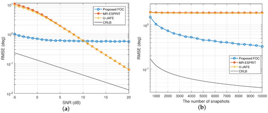
Figure 1.
RMSE of the DOA estimates of three independent signals versus (a) SNR when and (b) N when dB. FOC, fourth-order cumulants; MR, multiresolution; U, unitary.
Figure 2 depicts the RMSEs of the frequency estimates varying with changes of the SNR and snapshot size. Clearly, the proposed approach performed the best when the SNR was less than 7 dB or the number of snapshots exceeded 1500, whereas both U-JAFE and MR-ESPRIT were superior to our solution at moderate to high SNRs, and U-JAFE still achieved somewhat better accuracy of estimates than MR-ESPRIT under low SNRs, similar to the case of DOA estimation. Generally speaking, the proposed FOC-based method had a certain advantage over its second-order statistics counterparts in low SNR environments, whereas the latter provided better performance at high SNRs, which is consistent with the general results of the existing work. It should be noted that clear margins arose between the estimates, both DOA and frequency, and the CRLBs. This is mainly due to the fact that the cumulant-based estimator is inherently biased, and algorithms using second-order correlation are vulnerable to coloured noise, which will cause large estimation errors.
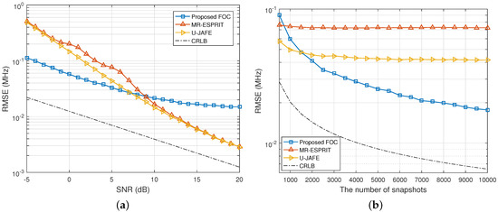
Figure 2.
RMSE of the frequency estimates of three independent signals versus (a) SNR when and (b) N when dB.
As discussed earlier, MR-ESPRIT, U-JAFE and the proposed FOC-based method were able to identify more independent signals than physical sensors, so it is necessary to investigate the performance of three approaches in such an underdetermined case. Assume that six independent sources from impinge on a five-element array (); the corresponding small frequency offsets for the signals are MHz, MHz, MHz, 2 MHz, MHz, 3 MHz, respectively, and the temporal smoothing factor . It can bee seen from Figure 3 that the absolute estimation performance of all techniques became worse, which is also illustrated by the CRLB, while the advantages of our technique over the other two became more obvious than the overdetermined case, and the counterparts U-JAFE and MR-ESPRIT only worked well above 19 dB and 20 dB, very large SNRs, respectively. Besides, the RMSE of the proposed FOC estimator approached the CRLB as the snapshot size increased, while both U-JAFE and MR-ESPRIT obtained almost the same large errors and remained constant throughout the numbers of snapshots, similar to Figure 1b.
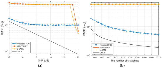
Figure 3.
RMSE of the DOA estimates of six independent signals versus (a) SNR when and (b) N when dB.
Figure 4 exhibits the performance of the three methods for the frequency estimation, as well as CRLB as a function of SNR and the total number of snapshots. One can observe that generally, the proposed method was distinctly better than the other two algorithms except at 20 dB and above, and U-JAFE outperformed MR-ESPRIT for all SNRs and snapshot sizes, which agrees with the results in Figure 2.
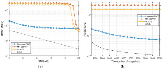
Figure 4.
RMSE of the frequency estimates of six independent signals versus (a) SNR when and (b) N when dB.
4.2. JAFE of Coherent Signals
In this section, we investigate the JAFE performance of the proposed cumulant-based algorithm first in the underdetermined coherent signals case, i.e., . It is assumed that two groups of six coherent signals uniformly distributed between and are imping on a six-element ULA, and the frequency offsets are MHz and MHz, respectively, as each group of coherent signals was derived from an independent source. The fading amplitudes of the coherent signals were and , while the fading phases were and , respectively. The temporal and spatial smoothing factors were and , and the SNR and number of snapshots were fixed at 15 dB and 5000. In such a scenario, neither U-JAFE nor MR-ESPRIT was able to resolve all DOAs as their DOFs were both upper bounded by four, whereas the proposed method can handle 20 DOAs at most. Figure 5a depicts the DOA estimation results of 50 independent trials by the proposed method. The solid lines mark the true DOAs. It can be seen that each DOA was correctly determined, and the frequency offset estimates were even more accurate, as shown in Figure 5b, since the DOFs used for the frequency estimation were larger than that for the DOA estimation.
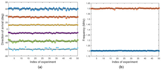
Figure 5.
Estimation results of groups of coherent signals via 50 runs in the underdetermined case. (a) DOA and (b) frequency versus the index of experiment when dB and .
Next, we examined the estimation performance of the proposed FOC-based estimator in the presence of multipath propagation. Assume that one group of coherent signals from arrives at a six-element array; the corresponding frequency offsets for the signals are 1.2 MHz, 1.6 MHz and 1.8 MHz, respectively. The fading amplitudes of the coherent signals were , while the fading phases were , respectively. The temporal and spatial smoothing factors were and , respectively. Figure 6 shows the RMSE of DOA estimates in the overdetermined case. It can be found that as the SNR and the number of snapshots increased, the RMSE of DOA estimation decreased gradually for all of the methods, where the accuracy of our algorithm improved asymptotically, whereas the RMSEs of U-JAFE and MR-ESPRIT were close to each other at low and moderate SNRs and tended to saturate at and , respectively. Evidently, the proposed FOC-based estimator was significantly superior to the counterparts for all SNRs and snapshot sizes tested, mainly because it exploited the dual rotational invariance of the frequency constructed by the rotation-invariant property in the generalized array manifold.
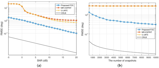
Figure 6.
RMSE of the DOA estimates of the group of coherent signals versus (a) SNR when and (b) N when dB.
In Figure 7, we plot the RMSEs of frequency estimates of the three methods as a function of SNR and the total number of snapshots under multipath propagation. It can be seen that the proposed solution had a prominent advantage over the other two algorithms for almost all the SNRs and snapshot sizes, although its lead kept decreasing as the SNR rose and turned out to be lost at 19 dB and above.Unlike the illustration in Figure 2, the performance of frequency estimation of U-JAFE was strictly worse than MR-ESPRIT over the whole range of SNR and snapshot size for coherent signal estimation. Additionally, the RMSEs of the frequency estimates by our method approached the CRLBs more tightly than the results in Figure 2 and Figure 4 since all three coherent signals shared an identical frequency, and the number of frequencies to be estimated turned out to be one less than the cases studied above.
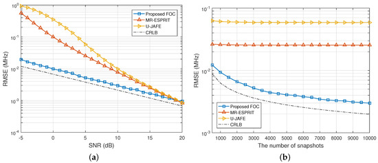
Figure 7.
RMSE of the frequency estimates of the group of coherent signals versus (a) SNR when and (b) N when dB.
5. Conclusions
The joint angle and frequency estimation of non-Gaussian signals in coloured noise is addressed in this paper, and cumulant-based estimation algorithms are developed for independent and coherent signals, respectively. The proposed methods make efficient use of the dual rotational invariance of the newly-constructed array manifolds to enhance the DOF of a ULA, thus improving the estimation accuracy and resolving more signals than the number of array elements, either for the independent or coherent signal. For independent signals, we construct an augmented cumulant matrix, providing twice the DOFs of the covariance matrix formed by the state-of-the-art techniques, then transform it to the real number field and resolve the DOA estimates by using rooting of a polynomial resulting from the RARE property, and the frequency estimates can be resolved in a least squares manner given the DOA estimates already acquired, avoiding the spatial spectra search and reducing the consumption of calculations accordingly. For coherent signals, the generalized steering vectors (coherent groups) and the frequencies are blindly separated from each other by exploiting a new dual rotational invariance arising from a series of dedicated cumulant matrices. Then, FBSS is performed to restore the inherent rank deficiency of the generalized steering vectors, and finally, the DOA estimates are determined by using the unitary ESPRIT algorithm. Since the coherent signals are divided and conquered, into their associated group, more coherent signals than array elements can be handled. Compared with previous second-order statistics methods, the proposed solutions are efficient in the sense that by extracting the temporal correlation embedded in the high-order statistics, they further raise the array DOFs and effective aperture, as well as improving the estimation accuracy, especially for coherent signals, in addition to the robustness to coloured noise.
Author Contributions
All authors contributed extensively to the study presented in this manuscript. Y.W. designed the main idea, methods and experiments, interpreted the results and wrote the paper. L.W. and B.W.-H.N. supervised the main idea, edited the manuscript and provided many valuable suggestions to this study. X.Y., J.X. and P.Z. carried out the experiments.
Funding
This work was supported in part by the National Key Research and Development Program of China under Grant 2018YFB0505104 and by the National Natural Science Foundation of China under Grants 61601372 and 61771404.
Acknowledgments
The authors would like to thank Matthew Trinkle from the University of Adelaide for his many constructive suggestions and comments that helped to improve the quality of the paper.
Conflicts of Interest
The authors declare no conflict of interest.
References
- Djeddou, M.; Belouchrani, A.; Aouada, S. Maximum likelihood angle-frequency estimation in partially known correlated noise for low-elevation targets. IEEE Trans. Signal Process. 2005, 53, 3057–3064. [Google Scholar] [CrossRef]
- Wang, S.; Caffery, J.; Zhou, X. Analysis of a joint space-time DOA/FOA estimator using MUSIC. In Proceedings of the IEEE International Symposium on Personal, Indoor and Mobile Radio Communications (PIMRC 2001), San Diego, CA, USA, 30 September–3 October 2001; pp. 138–142. [Google Scholar]
- Lin, J.D.; Fang, W.H.; Wang, Y.-Y.; Chen, J.T. FSF MUSIC for joint DOA and frequency estimation and its performance analysis. IEEE Trans. Signal Process. 2006, 54, 4529–4542. [Google Scholar] [CrossRef]
- Zoltowski, M.D.; Mathews, C.P. Real-time frequency and 2-D angle estimation with sub-Nyquist spatio-temporal sampling. IEEE Trans. Signal Process. 1994, 42, 2781–2794. [Google Scholar] [CrossRef]
- Haardt, M.; Nossek, J.A. 3-D unitary ESPRIT for joint 2-D angle and carrier estimation. In Proceedings of the 1997 IEEE International Conference on Acoustics, Speech, and Signal Processing (ICASSP), Munich, Germany, 21–24 April 1997; pp. 255–258. [Google Scholar]
- Lemma, A.N.; van der Veen, A.J.; Deprettere, E.F. Joint angle-frequency estimation using multi-resolution ESPRIT. In Proceedings of the IEEE International Conference on Acoustics, Speech and Signal Processing (ICASSP), Seattle, WA, USA, 15 May 1998; pp. 1957–1960. [Google Scholar]
- Lemma, A.N.; van der Veen, A.J.; Deprettere, E.F. Analysis of joint angle-frequency estimation using ESPRIT. IEEE Trans. Signal Process. 2003, 51, 1264–1283. [Google Scholar] [CrossRef]
- Zhang, X.; Feng, G.; Yu, J.; Xu, D. Angle-frequency estimation using trilinear decomposition of the oversampled output. Wirel. Pers. Commun. 2009, 51, 365–373. [Google Scholar]
- Liu, F.; Wang, J.; Du, R. Unitary-JAFE algorithm for joint angle-frequency estimation based on Frame-Newton method. Signal Process. 2010, 90, 809–820. [Google Scholar] [CrossRef]
- Kisliansky, A.; Shavit, R.; Member, S.; Tabrikian, J. Direction of arrival estimation in the presence of noise coupling in antenna arrays. IEEE Trans. Antennas Propag. 2007, 55, 1940–1947. [Google Scholar] [CrossRef]
- Niow, C.H.; Hui, H.T. Improved noise modeling with mutual coupling in receiving antenna arrays for direction-of-arrival estimation. IEEE Trans. Antennas Propag. 2012, 11, 1616–1621. [Google Scholar] [CrossRef]
- LeCadre, J. Parametric methods for spatial signal processing in the presence of unknown coloured noise fields. IEEE Trans. Acoust. Speech Signal Process. 1989, 37, 965–983. [Google Scholar] [CrossRef]
- Friedlander, B.; Weiss, A.J. Direction finding using noise covariance modeling. IEEE Trans. Signal Process. 1995, 43, 1557–1567. [Google Scholar] [CrossRef]
- Goransson, B.; Ottersten, B. Direction estimation in partially unknown noise fields. IEEE Trans. Signal Process. 1999, 47, 2375–2385. [Google Scholar] [CrossRef]
- Pesavento, M.; Gershman, A.B. Maximum-likelihood direction of arrival estimation in the presence of unknown nonuniform noise. IEEE Trans. Signal Process. 2001, 49, 1310–1324. [Google Scholar] [CrossRef]
- Vorobyov, S.A.; Gershman, A.B.; Wong, K.M. Maximum likelihood direction-of-arrival estimation in unknown noise fields using sparse sensor arrays. IEEE Trans. Signal Process. 2005, 53, 34–43. [Google Scholar] [CrossRef]
- Porat, B.; Friedlander, B. Direction finding algorithms based on high-order statistics. IEEE Trans. Signal Process. 1991, 39, 2016–2024. [Google Scholar] [CrossRef]
- Dǒgan, M.C.; Mendel, J.M. Applications of cumulants to array processing—Part I: Aperture extension and array calibration. IEEE Trans. Signal Process. 1995, 43, 1200–1216. [Google Scholar] [CrossRef]
- Chevalier, P.; Albera, L.; Ferreol, A.; Comon, P. On the virtual array concept for higher order array processing. IEEE Trans. Signal Process. 2005, 53, 1254–1271. [Google Scholar] [CrossRef]
- Wang, Y.; Trinkle, M.; Brian, B.W.H. Two-stage DOA estimation of independent and coherent signals in spatially coloured noise. Signal Process. 2016, 128, 350–359. [Google Scholar] [CrossRef]
- Yilmazer, N.; Koh, J.; Sarkar, T.K. Utilization of a unitary transform for efficient computation in the matrix pencil method to find the direction of arrival. IEEE Trans. Antennas Propag. 2006, 54, 175–181. [Google Scholar] [CrossRef]
- Bertsekas, D.P.; Nedić, A.; Ozdaglar, A.E. Convex Analysis and Optimization; Athena Scientific: Nashua, NH, USA, 2003. [Google Scholar]
- Pillai, S.U.; Kwon, B.H. Forward/backward spatial smoothing techniques for coherent signal identification. IEEE Trans. Acoust. Speech Signal Process. 1989, 37, 8–15. [Google Scholar] [CrossRef]
- Haardt, M.; Nossek, J.A. Unitary ESPRIT: How to obtain increased estimation accuracy with a reduced computational burden. IEEE Trans. Signal Process. 1995, 43, 1232–1242. [Google Scholar] [CrossRef]
- Ye, Z.; Zhang, Y. DOA estimation for non-Gaussian signals using fourth-order cumulants. IET Microw. Antennas Propag. 2009, 3, 1069–1078. [Google Scholar] [CrossRef]
- Wong, K.M.; Reilly, J.P.; Wu, Q.; Qiao, S. Estimation of the directions of arrival of signals in unknown correlated noise, part I: The MAP approach and its implementation. IEEE Trans. Signal Process. 1992, 40, 2007–2017. [Google Scholar] [CrossRef]
- Viberg, M.; Stoica, P.; Ottersten, B. Maximum likelihood array processing in spatially correlated noise fields using parameterized signals. IEEE Trans. Signal Process. 1997, 45, 996–1004. [Google Scholar] [CrossRef]
© 2019 by the authors. Licensee MDPI, Basel, Switzerland. This article is an open access article distributed under the terms and conditions of the Creative Commons Attribution (CC BY) license (http://creativecommons.org/licenses/by/4.0/).