Article

Intelligent Airflow Controls for a Stalling-Free Operation of an Oscillating Water Column-Based Wave Power Generation Plant

1
Automatic Control Group—ACG, Department of Automatic Control and Systems Engineering, Engineering School of Bilbao, University of the Basque Country (UPV/EHU), 48012 Bilbao, Spain
2
Laboratory of Research in Automatic Control—LA.R.A., National Engineering School of Tunis (ENIT), University of Tunis El Manar, BP 37, Le Belvédère, Tunis 1002, Tunisia
*
Author to whom correspondence should be addressed.
Electronics 2019, 8(1), 70; https://doi.org/10.3390/electronics8010070
Submission received: 15 November 2018 / Revised: 19 December 2018 / Accepted: 3 January 2019 / Published: 8 January 2019
(This article belongs to the Special Issue Intelligent Modelling and Control in Renewable Energy Systems)

Abstract

:
Control engineering in renewable energy systems is a delicate and tedious task, especially due to the unpredictable nature of the renewable resources, which requires precision and robustness. These requirements can be ensured using intelligent control, which provides better performance than many conventional techniques and methods. This paper focuses on the modeling and the intelligent control of the NEREIDA wave power plant of Mutriku in Spain. In this context, the design of two novel intelligent airflow controls for a stalling-free operation of the Wells turbine-based power take-off system is presented and compared. The airflow control will ensure the avoidance of the stalling behavior using an intelligent PID controller. The first control design methodology is based on the metaheuristic algorithms to ensure the optimization of the controller gains. The second methodology is based on the fuzzy gain scheduling of the gains. Two study cases were performed to compare the optimized-PID and FGS-PID to a conventional PID in two wave conditions. The results show the superior performance of both proposed controls over the conventional PID, providing power generation improvement in regular and irregular waves.

1. Introduction

Oceans and seas hold large quantities of stored energy from the Sun, which can be harnessed in various forms; thus, they are potentially able to play an important role in supplying clean energy [1]. Amongst the countless ocean energy converters, wave and tidal energy converters are expected to supply the most to the European energy mix in the short to medium term [1,2]. Power extracted from waves is a form of ocean power that has the uppermost exploitation potential in European seas, estimated to have a global potential 30-times superior to that of tidal energy [2]. This has attracted interest toward wave energy, leading countries to assess wave energy resources such as Hawaii, Italy, India, Peru, and many other countries around the world [3,4,5,6]. Even more, governments in some countries have set new guidelines to coordinate and facilitate the development of wave energy, such as the Wave Energy Scotland Agency established in Scotland in November 2014 [7].
The wave energy industry is increasingly proposing converters that incorporate hardware and software schemes and necessitate merging the expertise of multiple disciplines. Among the different kinds of wave energy technologies, the Oscillating Water Column (OWC) system is the most mature and the most investigated in the past. In Europe, there exist three main onshore facilities of OWC plants (see [2,8]). To operate these types of stations, there is the need to combine disciplines ranging from automatic control and power electronics to industrial informatics and metaheuristics. Such a complex scheme calls for the need of intelligent and advanced controls to respond to all needs and constraints.
The NEREIDA project, presented in Figure 1, is a wave power generation plant that was installed by the Basque Energy Agency (EVE) in the breakwater of Mutriku located in the northern Basque coast of Spain [9]. This station harnesses the wave energy through 16 OWC units. The PTO system of each OWC contains a Doubly-Fed Induction Generator (DFIG) of 18.5 kW, driven by a Wells turbine, giving an overall installed capacity of 296 kW [10]. The turbo-generator module is separated from the capture chamber by a throttle valve controlled by a PID controller. This allows the control of airflow and the shutdown in case of emergency closure situation (see Figure 1b). The main hurdle with Wells turbine-based PTO systems is the power limitation imposed by the stalling phenomenon of the turbine [11,12].
PID controllers are the most exploited and implemented controllers in industrial applications. Although PID controllers are robust versus uncertainties and structural variations in the plant parameters, their performance can be altered by such variations. Moreover, conventional PID tuning techniques are frequently founded on intricate and time-consuming trial-and-error experimental processes. Furthermore, with no proper systematic design method, the tuning procedure tends to be delicate and tedious.
The research work discussed in this article has a two-fold objective: on the one hand, to propose a control strategy to avoid the power limitation imposed by the stalling phenomenon and, on the other hand, to improve the limitations of the conventionally-tuned PID controller using intelligent design methodologies against the wave changes at the site of Mutriku. In this context, a novel airflow control is proposed to govern a throttle valve to help adjust the airflow in the turbine duct. Two control design methodologies have been suggested to ameliorate the performance of the basic airflow control scheme. The first approach is by tuning the PID controller gains using advanced metaheuristic algorithms, in particular the Harmony Search Algorithm (HSA). The second approach is the fuzzy gain scheduling technique using the fuzzy supervisor to change the gains adaptively.
The remainder of this paper is organized as follows; Section 2 provides a brief wave background and a wave model. Then, the OWC topology is described and modeled in Section 3. Section 4 presents the problem statement explaining the stalling behavior of the Wells turbine and its effect on the produced torque and the generated power. Section 5 is dedicated to the control statement, detailing two control design methodologies for the airflow control strategy. The first method is based on advanced metaheuristic algorithms with emphasis on the Harmony Search Algorithm (HSA), and the second method is the Fuzzy Gain Scheduling (FGS) technique. Section 6 gives two demonstrative study cases to investigate the effectiveness of both HSA-tuned PID- and FGS-PID-based airflow control in regular and irregular waves. Finally, Section 7 finishes the paper with some concluding remarks.

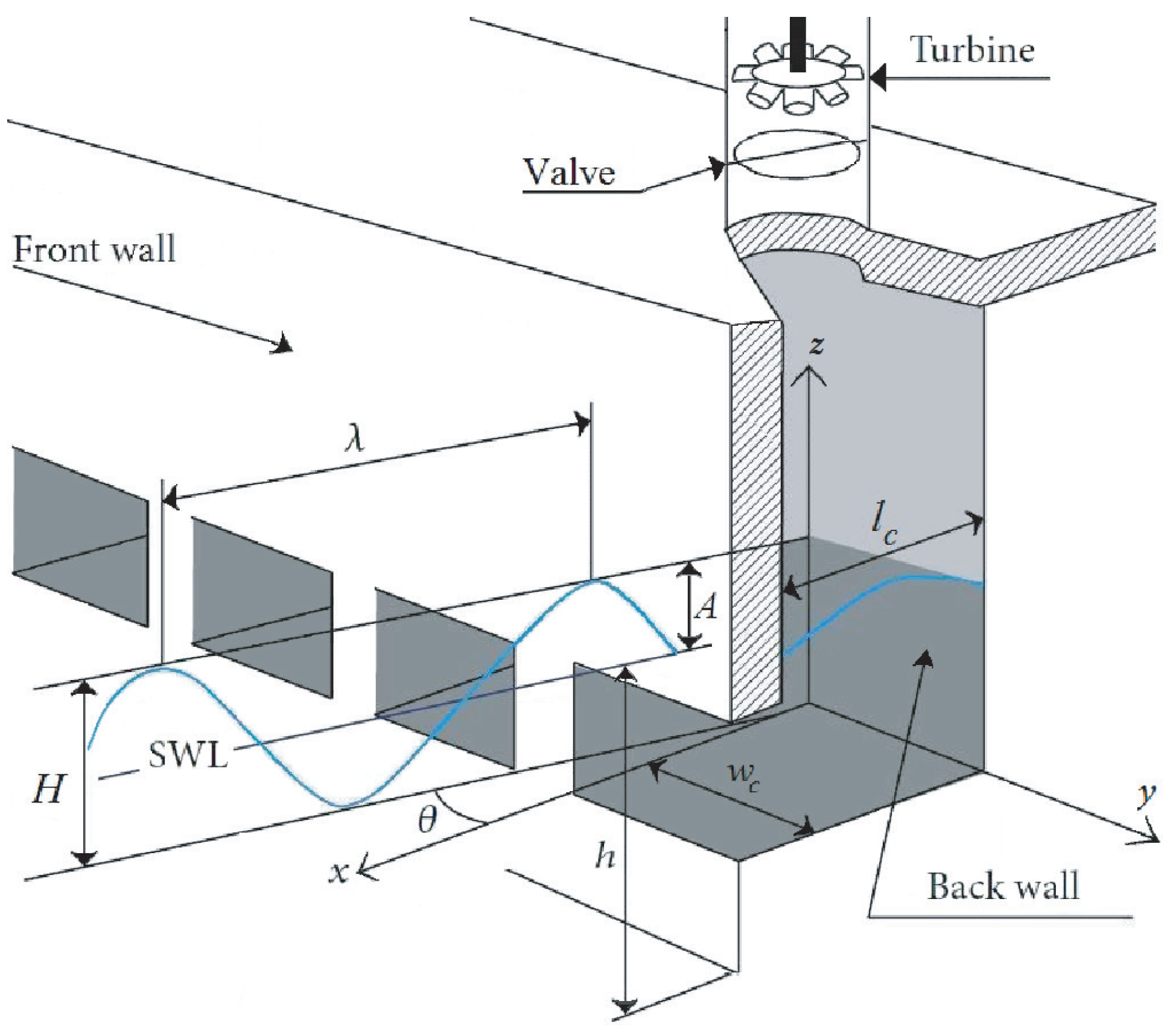
2. Wave Background and Model

Researchers have proposed and applied many wave theories [13,14,15,16,17,18,19] because describing and modeling the water particle kinematics of ocean waves is a complex task. The proposed theories vary from the Airy wave theory, Stokes second-order and other higher order theories, cnoidal wave theory to stream-function wave theory [13,14,15,16,17,18,19]. The simplest expression of ocean waves is attributed to the Airy theory in 1845, which is sufficiently accurate for many engineering purposes [19].
The Airy wave theory commonly referred to as linear wave theory or first-order wave theory has been considered because it is applicable to describe shallow waters. Hence, the wave model can be expressed as regular sine waves thanks to the simplifying assumptions made in its derivation, which neglects turbulence, friction losses, and other energy losses [19]. To set an adequate wave model relative to the site of Mutriku, wave parameters, characteristics, and specific data from the location of the wave power plant are required. Figure 2 illustrates the outline of the waveform of an ocean wave, where SWL is the Still Water Level and h is the sea depth from the seabed to SWL. H is the wave height from the wave trough to the wave crest. A is the wave amplitude from SWL to the wave crest, and λ is the wavelength, which is the distance between successive crests [13].
Hence, the surface elevation of an ocean wave may be written as [20,21]:
z ( x , t ) = A sin ω t k x θ = H 2 sin ω t k x θ
where k is the wave number, x is a horizontal coordinate whose positive direction is the direction of wave propagation, with x = 0 at the back wall, and θ is the angle between the x-axis and the direction of wave advance.
The wave number k is related to ω by the dispersion relationship (2) defined in [20].
k tanh ( k h ) = ω 2 ω 2 g g
where ω is the wave frequency and g is the acceleration gravity.
In the literature, a realistic irregular wave can be expressed by the superposition of a finite number of regular waves and written as [8,21]:
z ( x , t ) = n = 1 N A n sin ω n t k n x + θ n
where N is a finite number of regular waves.
To select the appropriate wave amplitude A and wave period T w for the wave model, the spectrum of the wave climate at the site needs to be taken into account. A wave spectrum indicates the amount of wave energy as a function of the wave frequency. A representative spectral analysis of the waves at the site of Mutriku on 12 May 2014 is shown in Figure 3 [18].
It may be seen from Figure 3 that the waves at Mutriku are concentrating around three distinct frequencies, 0.08 Hz, 0.15 Hz, and 0.23 Hz, which corresponds to the periods 12.5 s, 6.66 s, and 4.34 s, respectively. This will help us to implement and test the wave model.

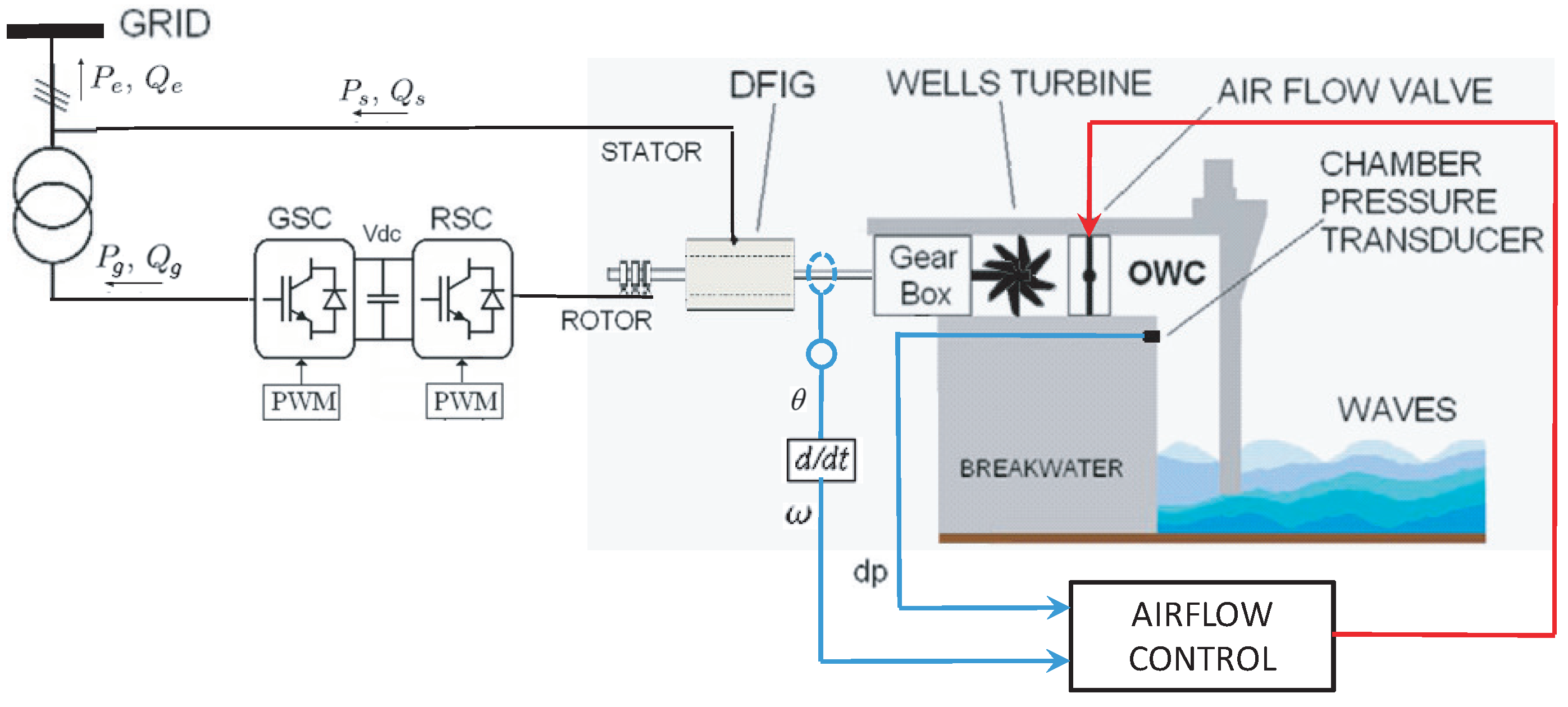
3. OWC Plant Modeling

3.1. Capture Chamber Model

The volume of the water entering the chamber from the bottom opening can be used to express the volume of the air oscillating in and out of the chamber from the turbine duct at the top as [18,22,23,24]:
V ( t ) = V c V w ( t )
where V c and V w are the chamber and water volumes.
Integrating the orthogonal deviation of the water’s surface along the area of the chamber, Equation (4) becomes [18,22,23]:
V ( t ) = V c z ( x , t ) . d S
By considering the capture chamber’s geometry at Mutriku, we get [18,22,23]:
d S = w c d x
where w c is the inner width of the chamber.
Finally, when integrating the air volume Equation (5), it develops into [18,22,23,24]:
V ( t ) = V c + w c H k sin k l c 2 sin ( ω t )
where l c is the length of the capture chamber.
From (7), the volume flow rate may be described as [18,22,23]:
Q ( t ) = w c c H sin k l c 2 cos ( ω t )
Furthermore, by using (8) and taking into consideration the topology of the capture chamber, the axial airflow speed may be defined as [18,22,23]:
v x ( t ) = Q ( t ) S = 8 A c w c π D 2 sin π l c c T w cos 2 π T w t

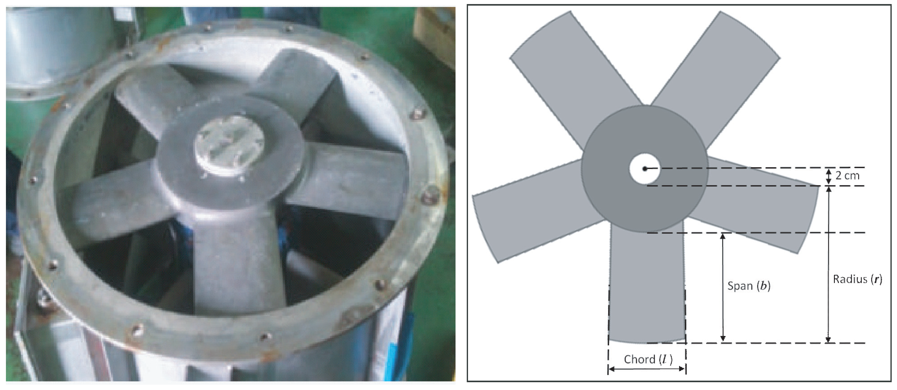
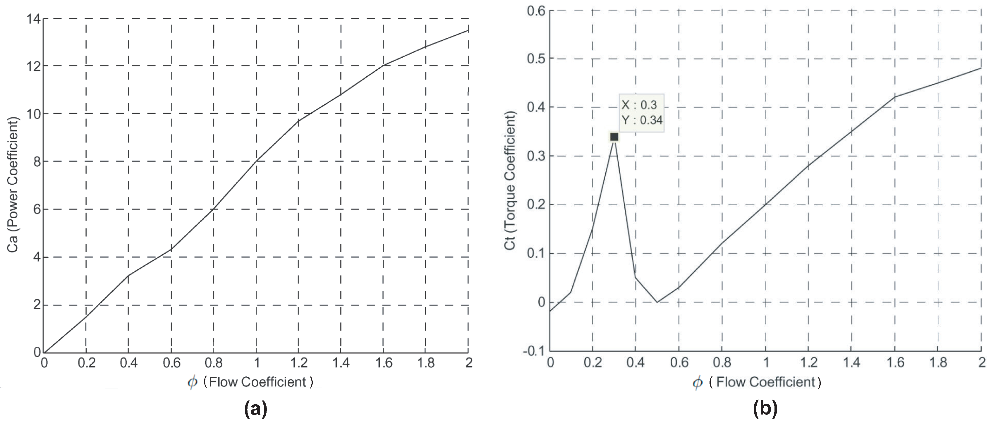
3.2. Wells Turbine Model

The airflow in the turbine duct will serve as the input to the Wells turbine model. The turbine under study shown in Figure 4 was invented by Dr. Allan Wells in the mid-1970s [25] and is a self-rectifying axial-flow turbine [26,27,28].
The Wells turbine may be described by the equations given in [12,14,29] to model the interaction between the ocean waves and the OWC plant.
The pressure drop across the turbine rotor is defined (in Pa) as:
d p = C a K 1 1 a a v x 2 + r ω r 2
where a is the cross-sectional area, C a is the power coefficient, r is the mean radius, ω r is the angular velocity, and K is the turbine constant (in kg/m) defined as:
K = ρ l b n 2
where ρ is the air density, l is the blade chord length, b is the blade height, and n is the number of blades.
The torque obtained from the turbine may be expressed as:
T t = r C t K v x 2 + r ω r 2
where C t is the torque coefficient.
The relation between the torque and the pressure drop may be defined as:
T t = r a C t C a d p
The flow coefficient of the Wells turbine can be expressed as:
ϕ = v x r ω r 1
The expression of the flow rate can be defined as:
Q = a v x
Lastly, the turbine efficiency may be written as:
η t = T t ω r d p Q 1 = C t C a ϕ 1
The curves of both the power coefficient C a and the torque coefficient C t against the flow coefficient ϕ form the characteristic curves of the studied Wells turbine, which are presented in Figure 5a,b. These curves will be used to compute the turbine torque and generated power [18,22,23].

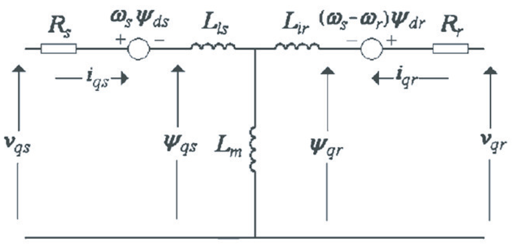
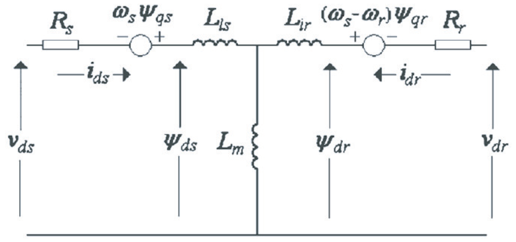
3.3. Doubly-Fed Induction Generator Model

The mechanical power produced by the turbine drives the DFIG to supply electricity to the grid. In a d-q biphase frame, Figure 6 and Figure 7 show the equivalent circuit of the DFIG in the d-axis and q-axis [18,22,23].
Hence, the DFIG model may be described by the equations given in [30,31,32].
The voltages across the stator and rotor in the d-q frame may be written as [22,23,30,31,32]:
v d s = R s i d s + d ψ d s d t ω s ψ q s v q s = R s i q s + d ψ q s d t + ω s ψ d s
v d r = R r i d r + d ψ d r d t ω r ψ q r v q r = R r i q r + d ψ q r d t + ω r ψ d r
where R s and R r are the stator and the rotor resistances, ω s and ω r are the stator and the rotor angular velocity, i d s and i q s are the d-q stator currents, and i d r and i q r are the d-q rotor currents.
The flux linkage in the stator and the rotor may be written as:
ψ d s = L s s i d s + L m i d r ψ q s = L s s i q s + L m i q r
ψ d r = L r r i d r + L m i d s ψ q r = L r r i q r + L m i q s
where L s s and L r r are the stator and the rotor inductances and L m is the magnetizing inductance.
The generated electromagnetic torque may be expressed as:
T e = 3 2 p ψ d s i q s ψ q s i d s
where p is the pair pole number.
The mechanical interaction between the turbine and the generator can be defined as:
J p d ω r d t = T e T t
where J is the inertia of the system.

3.4. Back-to-Back Converter Model

The power generated by the DFIG will be delivered to the grid through the back-to-back converter. In this context, a description and a model of the converter are presented.
The AC-DC-AC converter contains a Grid-Side Converter (GSC) wired to the grid and a Rotor-Side Converter (RSC) wired to the wound rotor windings [33,34]. Both of the converters are joined back-to-back by a DC-link capacitor, as illustrated in Figure 10.
The role of the RSC is applying the voltages at the rotor windings of the DFIG. It is intended to control the rotor currents in order to get the rotor flux aligned with the stator flux so as to produce the required torque at the shaft of the machine. This will help adjust the voltages and the generated power measured at the stator [35].
The active and reactive power at the stator may be written as:
P s = 3 2 v d s i d s + v q s i q s
Q s = 3 2 v q s i d s v d s i q s
The system at the grid side is composed of a GSC, grid filter, and the DC bus capacitor. This side of the converter is intended to adjust the DC-link voltage and is able to generate or absorb reactive power to guarantee the DC voltage regulation [22,35].
The exchanged active and reactive powers between the GSC and the grid may be written as [22,35]:
P g = 3 2 v d g i d g + v q g i q g
Q g = 3 2 v q g i d g v d g i q g
Here, v d g and v q g are the d-q components of the grid voltages and i d g and i q g are the d-q components of the grid currents.
The DC-link model describes the voltage variations of the capacitor as a function of the received power at the bus [35,36]. The energy stored in the capacitor can be expressed as:
W d c = P d c d t = 1 2 C v d c 2
where C is the capacitance, v d c is the capacitor’s voltage, W d c is the stored energy, and P d c is the input power to the DC-bus.
The derivatives of the voltage and energy at the DC-bus may be expressed as:
d v d c d t = P d c C v d c
d W d c d t = P d c
The DC-link power may be computed as:
P d c = P R S C P G S C
Hence, the voltage at the DC-link varies as the power P d c changes and is constant when P d c is zero. Whether the DFIG is absorbing ( P d c < 0 ) or injecting ( P d c > 0 ) power from/to the grid, the variation of P d c will vary the derivative of the voltage. This explains the need to regulate v d c in order to keep P d c positive and constant [35].

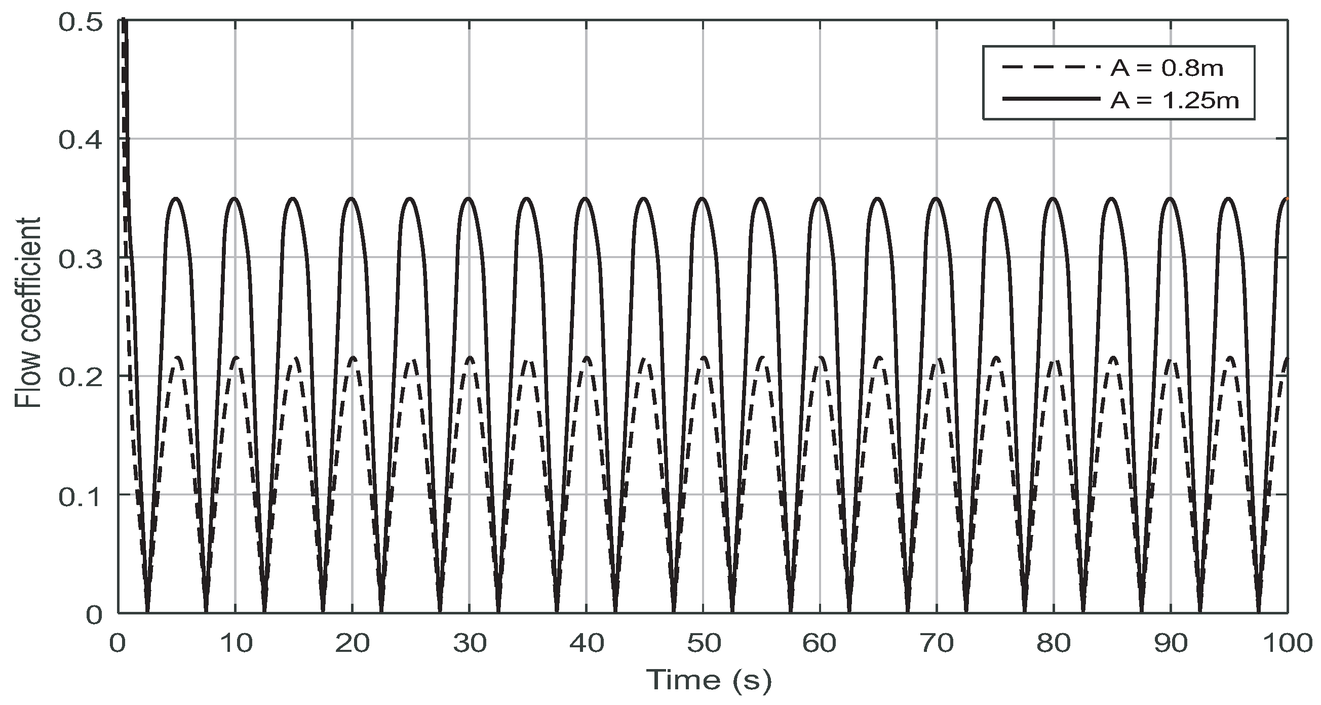
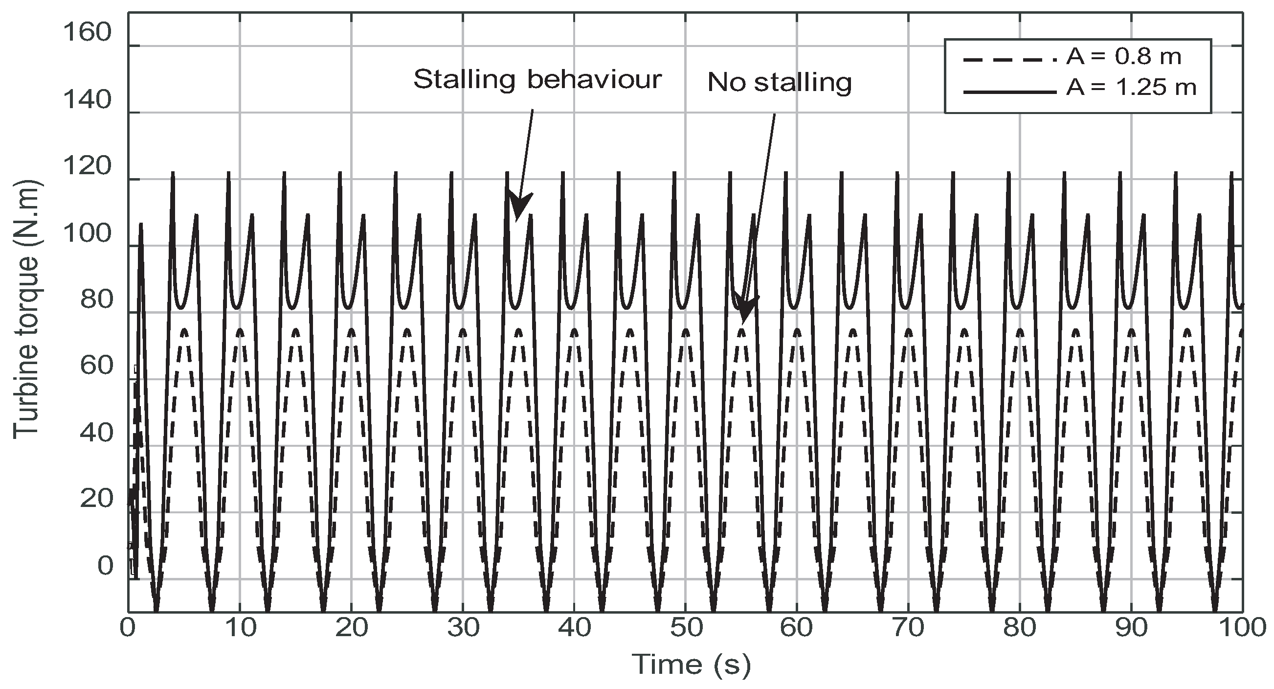
4. Problem Statement

The stalling phenomenon of the Wells turbine is a feature that limits the generated power. This behavior has been described by Equation (14); in fact, it arises as the airflow speed augments, but the rotational speed is low because the DFIG is not capable of rotating quick enough to keep up with the incoming airflow. Figure 5 shows that if the flow coefficient ϕ exceeds a critical value 0.3 , the torque coefficient C t will decrease significantly due to the rotational speed ω r not keeping up with the axial flow speed v x .
To further comprehend the stalling phenomenon and its effect, an investigation of the OWC plant in two sea conditions has been performed. The results of the study on the flow coefficient and the turbine torque are presented in Figure 8 and Figure 9 [22,23].
The first sea state considers waves with an amplitude of 0.8 m and a wave period T w = 10 s; this condition will result in a flow coefficient lower than the threshold value 0.3 . Accordingly, no stalling behavior takes place in the produced torque as shown by both dashed curves of Figure 8 and Figure 9. However, the second sea state considers waves with an amplitude of 1.25 m and a wave period T w = 10 s; this scenario will result in a flow coefficient that exceeds the threshold value 0.3 . Consequently, the stalling behavior takes place and affects the obtained turbine torque, reducing its average value, as shown by the continuous curve of Figure 9.

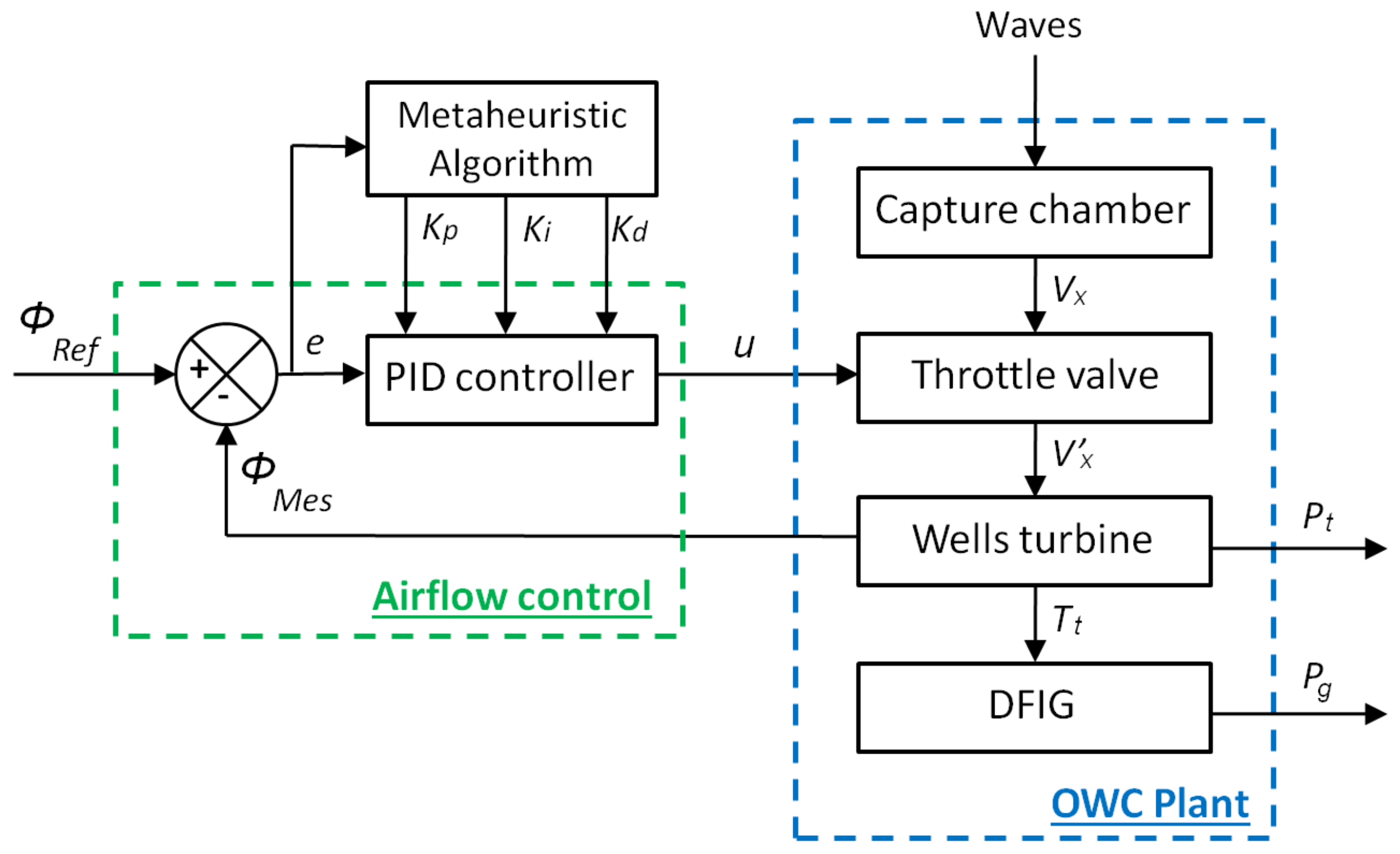
5. Control Statement

The stalling phenomenon may be avoided if the axial flow velocity v x is regulated; this will prevent the flow coefficient ϕ from surpassing the threshold value 0.3 . By referring to Equation (14), this adjustment is feasible by governing the throttle valve in the turbine duct, as indicated in the airflow control scheme of Figure 10.
The suggested airflow control scheme uses a PID controller to control the opening of the throttle valve, which will adjust the airflow in the turbine duct. This is accomplished via measurements of the rotational speed and pressure drop from which the axial flow speed and the flow coefficient are computed. The flow coefficient is then compared to the reference flow coefficient ϕ r e f , which in this case is the threshold value 0.3 . The control signal is fed to a PWM module as the image of the duty cycle; hence, the control signal could be adapted to a value between 0 and 5 V if the TTL technology is used or between 0 and 15 V if IGBTs are used. The PWM module will control an H bridge to supply voltage to the DC motor rotating the throttle disc. Consequently, the valve is able to rotate its throttle disc to the desired angular opening. This will ensure the appropriate angular position to regulate the axial flow speed v x .
Although PID controllers are robust versus uncertainties and structural variations in the plant parameters, their performance can be altered by such variations; hence the necessity of optimally-tuned gains emerged to help maintain the required performance. In this context, two design methodologies were adopted and implemented to improve the performance of a traditionally-tuned PID controller. The first approach is based on metaheuristic algorithms to obtain the optimal value of the gains, and the second approach is based on the fuzzy gain scheduling technique to regulate the gain values adaptively.

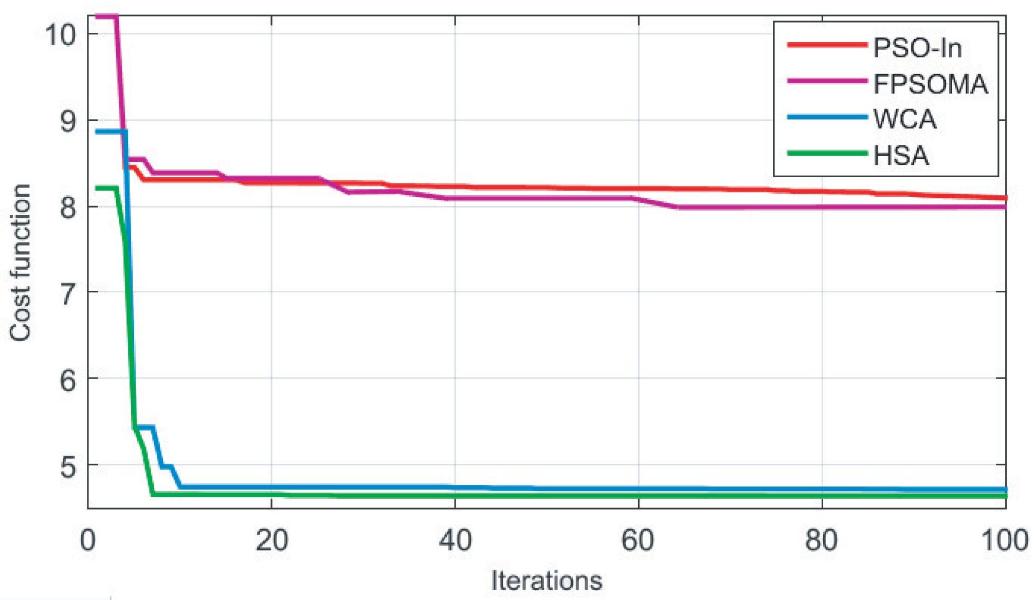
5.1. Metaheuristic-Based Airflow Control

5.1.1. Control Problem Formulation

Traditional PID tuning techniques are frequently founded on intricate and time-consuming trial-and-errors experimental processes. Additionally, with no proper systematic design method, the tuning procedure tends to become delicate and tedious. To deal with these design difficulties, the optimization theory is shown to be a successful approach to compute and optimize easily the PID parameters [37,38,39,40,41]. Many advanced metaheuristic algorithms have been studied and tested with different PID structures, controllers, and applications such as the Particle Swarm Optimization with decreasing Inertia (PSO-In) [42,43], the Fractional Particle Swarm Optimization Memetic Algorithm (FPSOMA) [42,43], and the Water Cycle Algorithm (WCA) [44,45].
The optimization problem of the PID tuning within the airflow strategy scheme aims to determine the control design parameters x * = x 1 * , x 2 * , x 3 * T R 3 which corresponds to the PID controller gains, i.e., x = K p , K i , K d T R + 3 , by minimizing the cost function, which have been chosen in this case as the Integral of Absolute Error (IAE) [22,23,43]:
f I A E x = 0 + e x , t d t
where e . represents the instantaneous error between the reference and the controlled plant output, as shown in Figure 11.
The objective function is minimized by taking into consideration a number of time-domain constraints, which are related to the steady-state error E s s , the rise time t r , the settling time t s , and the overshoot δ % criteria of the closed-loop step response [22,23,37].
The tuning problem concerning the airflow strategy for the oscillating water column system may be described by the constrained and nonlinear optimization formulation of Equation (32). This will be solved using the metaheuristic algorithms [22,23]:
m i n i m i z e f x x = K p , K i , K d T S R + 3 subject to : g 1 x = E s s E s s max 0 g 2 x = t r t r max 0 g 3 x = t s t s max 0
where f : R 3 R is the objective function, S = x R + 3 , x l o w x x u p p e r represents the bounded search space for the decision variables, and g i : R 3 R , i = 1 , 2 , 3 are the problem constraints. E s s max , t r max and t s max are the pre-specified maximum values for steady-state error, rise, and settling times, respectively.
A variety of methods have been suggested to deal with the constraints of problems such as Problem (32). The most common technique is applying penalties to the objective function. In this context, an external static penalty technique has been considered and is described as [38,39]:
φ x = f x + j = 1 n c o n Λ j max 0 , g j x 2
where Λ j are the scaling penalty parameters and n c o n is the number of constraints.
In a standard optimization process, the scaling parameters Λ j , used in Equation (33), will be linearly increased at every iteration step in order to enforce the constraints gradually. Usually, the quality of the obtained solutions is directly dependent on the specified values of the scaling parameters. In this work and to render the suggested method simple, large and constant scaling penalty parameters are considered [22,23,38].
In fact, the second term of Expression (33) augments the cost function of Problem (32) by static penalties, which are proportional to the level of constraint infeasibility, which means that the better the solution is when taking into consideration g j , the less penalties are applied, and therefore, it is maintained. However, the worse the solution obtained is, the more penalties are applied in order to reject it [22,23].

5.1.2. Harmony Search Algorithm

The Harmony Search Algorithm (HAS) was inspired by the musical process in the search for a fantastic harmony [46]. The HSA algorithm finds the finest musical state by aesthetic estimation [47,48,49].
A typical HSA executes the basic steps detailed below [49]:
  • Step 1: Initializing the Harmony Memory (HM) arbitrarily with:
    H M = x 1 1 x 2 1 x n 1 x 1 2 x 2 2 x n 2 x 1 H M S x 2 H M S x n H M S
    Here, x i = x 1 i , x 2 i , , x n i is a possible solution, and H M S is the size of the HM.
  • Step 2: Improving a new solution x i = x 1 i , x 2 i , , x n i from the harmony memory.
    The decision variables are determined by using the Harmony Memory Consideration Rate (HMCR) parameter described as the probability P HMCR to select an element from the HM [47,48,49].
    x j x j 1 , x j 2 , , x j H M S , with probability P HMCR x j X j , with probability 1 P HMCR
    where X j is the set of possible range of values for each decision variable.
    A Pitch Adjustment (PA) procedure will examine each element determined by the HMCR parameter to decide whether it should go under a pitch adjustment process using the Pitch Adjusting Rate (PAR) parameter described as the probability P PAR to mutate a candidate solution from the HM [47,49].
    P A x j = y e s with probability P PAR n o with probability 1 P PAR
  • Step 3: Updating the harmony memory. New solutions from Step 2 are assessed. In fact, if the solution offers a better cost function compared to that of the worst component in the harmony memory, then the new solution will replace the worst element. Otherwise, it is discarded.
  • Step 4: Abort executing when the termination condition is reached. Else, return to Step 2.

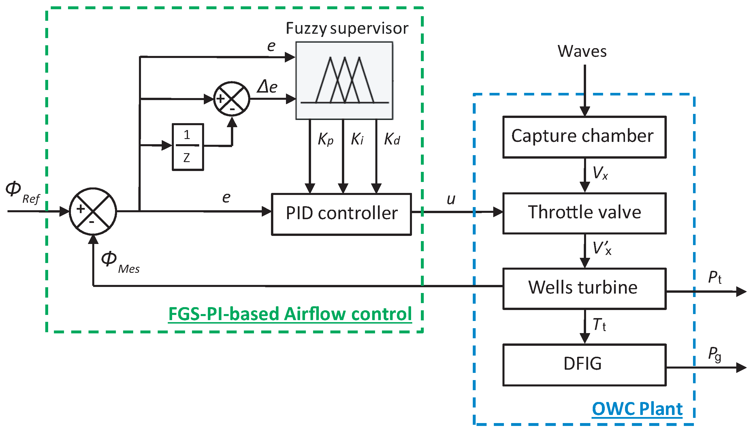
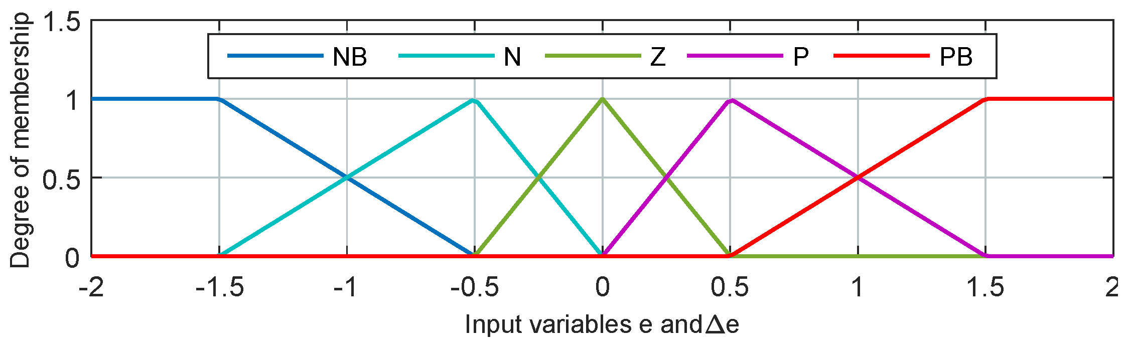
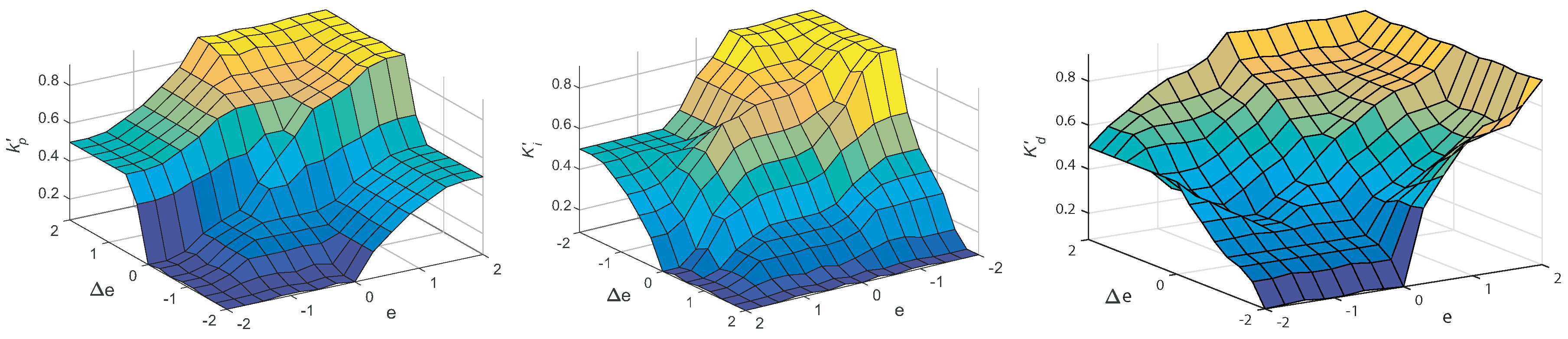
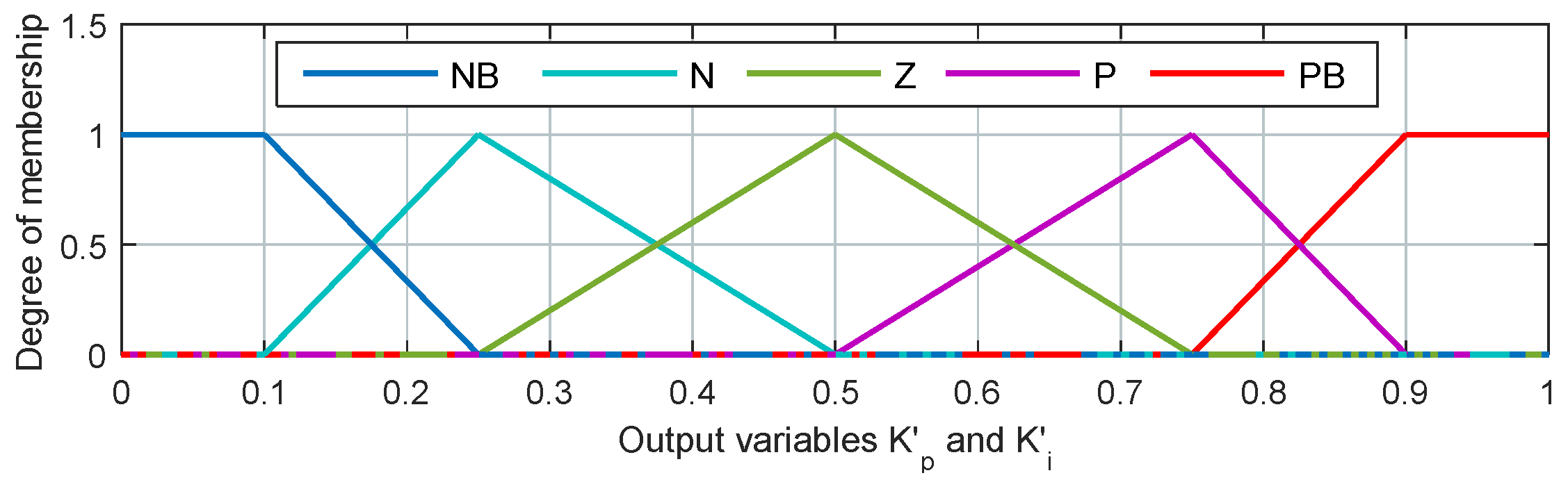
5.2. Fuzzy Gain Schedule-Based Airflow Control

To overcome the drawback of a traditionally-tuned PID controller, the Fuzzy Logic Controller (FLC) is used to tune PID gains online where the tracking error and the change of the tracking error are used to determine control parameters. The idea of Fuzzy Gain Scheduled PID (FGS-PID) was first introduced by Zhen-Yu Zhao et al. in 1993 [50]. Since then, many applications embraced this tuning method, including renewable energy converters [51,52,53].
The gains of the PID controller are determined using a fuzzy supervisor based on fuzzy rules and reasoning. This way, the PI gains are no longer fixed values; in fact, the gains vary relative to the error’s evolution.
Figure 12 illustrates the FGS-PID-based airflow control scheme proposed for the OWC plant. The input to the controller is the error between the reference flow coefficient ϕ R e f and the measured flow coefficient ϕ M e s .
The expression of the PID controller in discrete-time is given as:
u ( k ) = u ( k 1 ) + K p Δ e ( k ) + K i T s e ( k ) + K d Δ e ( k )
where u ( k ) is the control signal, T s is the sampling period, e ( k ) is the error between the reference and the process output, Δ e ( k ) is the change of error defined as Δ e ( k ) = e ( k ) e ( k 1 ) , and K p , K i , and K d are, respectively, the proportional, integral, and derivative gains.
The fuzzy inference system that has been considered has two inputs and three outputs, K p , K i , and K d gains, as illustrated in Figure 13. It is assumed that the parameters K p , K i , and K d are in the prescribed ranges K p min , K p max , K i min , K i max , and K d min , K d max , respectively.
The PID controller parameters are calculated using the well-known normalization method as given in [50] as follows:
K p = K p K p min K p K p min K p max K p min K p max K p min
K i = K i K i min K i K i min K i max K i min K i max K i min
K d = K d K d min K d K d min K d max K d min K d max K d min
where K p , K i , and K d are the fuzzy outputs obtained from the fuzzy rules for gain scheduling, which are defined in the form of IF-THEN as:
if ( e i s A i a n d Δ e i s B i ) then ( K p i s C i a n d K i i s D i a n d K d i s E i )
where A i , B i , C i , D i , and E i are the fuzzy sets on the corresponding fuzzy sets with i = 1 , 2 , ... , m .
The membership functions for the inputs e and Δ e of the fuzzy supervisor are described with the fuzzy sets A i and B i , which are characterized by the membership functions of Figure 13. Triangular and trapezoidal membership functions are used for input variables on the universe of discourse. The linguistic levels are Negative Big (NB), Negative (N), Zero (Z), Positive (P), and Positive Big (PB).
The membership functions for the output variables K p , K i , and K d are described with the fuzzy sets C i , D i , and E i , which are characterized by the membership functions of Figure 14.
Triangular and trapezoidal membership functions are used as well for output variables, and the linguistic levels are also NB, N, Z, P, and PB.
Hence, the grade of the membership functions μ A i and μ B i is defined as:
μ N B X = 1 if X 3 2 ( 1 2 X ) if X ( 3 2 , 1 2 ) 0 if X 1 2 μ N X = 0 if X 3 2 ( X 2 3 4 ) if X ( 3 2 , 1 2 ] 2 X if X ( 1 2 , 0 ) 0 if X 0 μ Z X = 0 if X 1 2 ( 2 X + 1 ) if X ( 1 2 , 0 ] ( 1 2 X ) if X ( 0 , 1 2 ) 0 if X 1 2 μ P X = 0 if X 0 2 X if X ( 0 , 1 2 ] ( 3 2 X ) if X ( 1 2 , 3 2 ) 0 if X 3 2 μ P B X = 0 if X 1 2 ( X 1 2 ) if X ( 1 , 2 ] 1 if X 3 2
where X is e or Δ e .
The grade of the membership functions μ C i , μ D i , and μ E i is defined as:
μ N B X = 1 if X 3 4 ( 4 X 2 ) if X ( 3 4 , 1 2 ) 0 if X 1 2 μ N X = 0 if X 3 4 ( 4 X + 3 ) if X ( 3 4 , 1 2 ] 2 X if X ( 1 2 , 0 ) 0 if X 0 μ Z X = 0 if X 1 2 ( 2 X + 1 ) if X ( 1 2 , 0 ] ( 1 2 X ) if X ( 0 , 1 2 ) 0 if X 1 2 μ P X = 0 if X 0 2 X if X ( 0 , 1 2 ] ( 3 4 X ) if X ( 1 2 , 3 4 ) 0 if X 3 4 μ P B X = 0 if X 1 2 ( 4 X 2 ) if X ( 1 2 , 3 4 ] 1 if X 3 4
where X is K p , K i , or K d .
Three sets of 25 rules, shown in Table 1, Table 2 and Table 3, are used in (41). These rules may be determined heuristically based on the desired time step response of the process [50]. In our case, we focus on having the behavior of a conventional PID controller, but adaptively changing when the plant is running according to the error e and the error variation Δ e .
The truth value of the ith rule in (41) is obtained by the product of the truth value of the components of the antecedent clauses as:
μ i = μ A i e k . μ B i Δ e k
By using the membership functions of Figure 14, we obtain:
i = 1 m μ i = 1
thus the defuzzification scheme is defined as:
K p = i = 1 m μ i . μ C i
K i = i = 1 m μ i . μ D i
K d = i = 1 m μ i . μ E i
The obtained fuzzy surfaces for K p , K i , and K d gains are given by the 3D plots of Figure 15.
The decision-making output is obtained using a Max-Min fuzzy inference where the crisp outputs are calculated by the center of gravity defuzzification method as:
K p = K p min + K p max K p min K p
K i = K i min + K i max K i min K i
K d = K d min + K d max K d min K d

6. Results and Discussion

This section presents the investigation carried out to evaluate the performance of both the HSA-based airflow control and the fuzzy gain scheduling-based airflow control. To evaluate the performance of both implemented control methodologies, a comparison to the uncontrolled case and the case of the conventionally-tuned PID has been performed. In this context, the Ziegler–Nichols (ZN) experimental method has been chosen in this investigation, since it is the mainly-used and well-known conventional tuning technique for PID controllers in industry applications [54,55].
For the implemented OWC system, we considered the parameters obtained from real measurements at the NEREIDA wave power plant. These parameters were provided by the Basque Energy Agency (EVE) and are detailed in Table 4.

6.1. Advanced PID Tuning and Setup

For the conventional PID controller, we tuned the gains using the second technique of the ZN-based experimental method [54]. After determining some preliminary values of the PI parameters using the ZN method, additional enhancements have been performed to ameliorate the controlled plant based on trial-and-error tests [55,56,57]. The gains obtained and considered were K p = 4800 , K i = 0.38 , and K d = 0.01 .
In the case of the fuzzy gain-scheduled PID, the gains of the PID were computed using the fuzzy supervisors. With the assumption that the parameters K p , K i , and K d were in the prescribed ranges K p min , K p max , K i min , K i max , and K d min , K d max , respectively, the predefined ranges of K p , K i , and K d for the fuzzy gain-scheduled PID in the airflow control were K p min = 180 , K p max = 8000 , K i min = 0.1 , K i max = 0.9 , and K d min = 0.001 , K d max = 0.9 .
In the case of the HSA-tuned PID, the same investigation has been carried out in previous works with the Particle Swarm Optimization with decreasing weight Inertia (PSO-In), the Fractional Particle Swarm Optimization Memetic Algorithm (FPSOMA), and the Water Cycle Algorithm (WCA) based on the identical parameters and scenarios, and the results found were presented in [22,23].
The results of the optimization-based PID tuning for the airflow control using all four algorithms are presented in Table 5. By comparing the results to that of the PSO-In, FPSOMA, and WCA, the HSA algorithm provided attractive results associated with a lower cost function.
The history of convergence of all four tested algorithms is illustrated by the curves of Figure 16. The convergence of the HSA proves that the algorithm effectively located an interesting area of the design search space to explore. Furthermore, compared to the other three implemented algorithms, it had the best results in terms of exploration and exploitation.
In this investigation, the simulation of the controlled plant has been carried out with the decision variables obtained from the mean case of optimization results by the HAS to set up the PID gains.

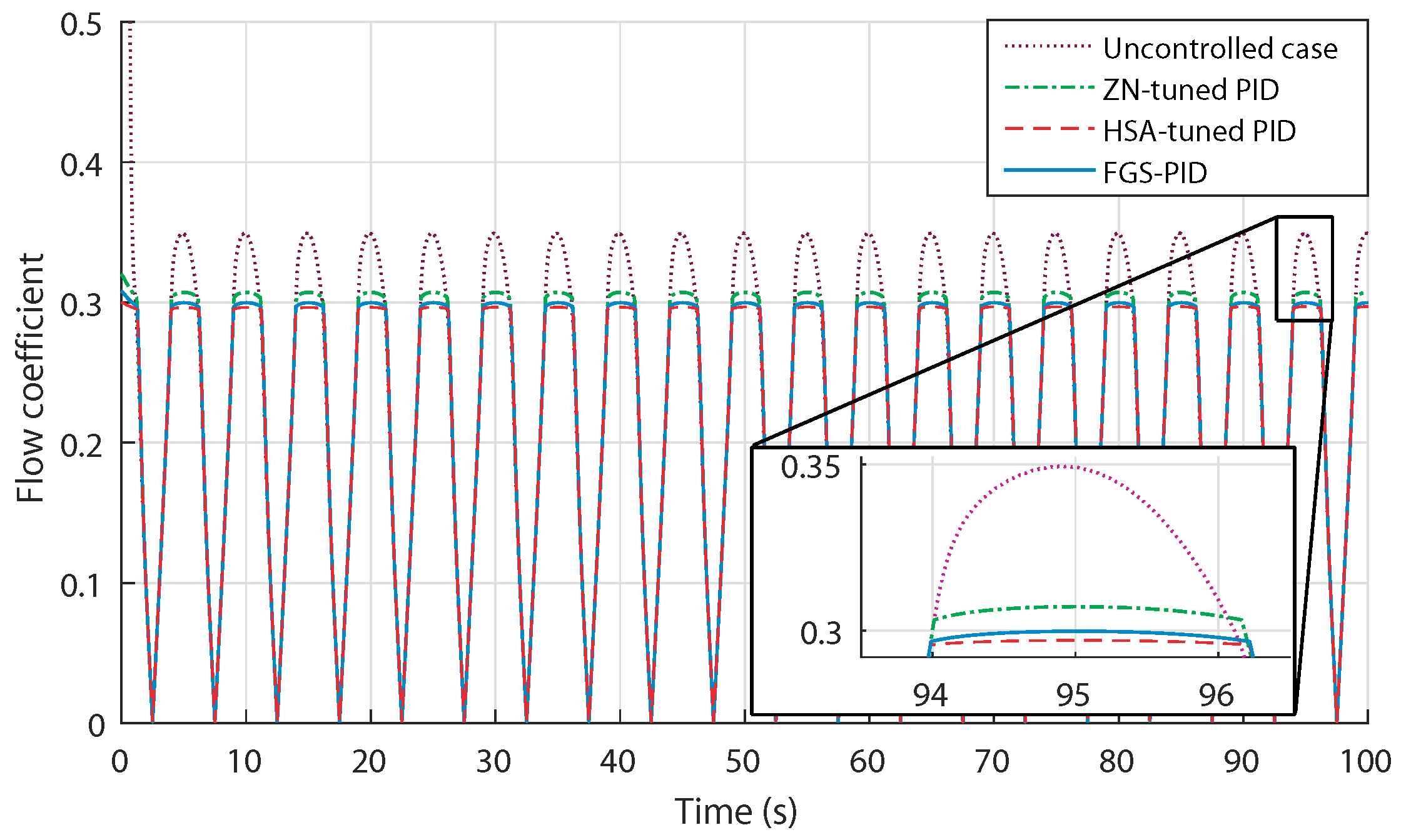
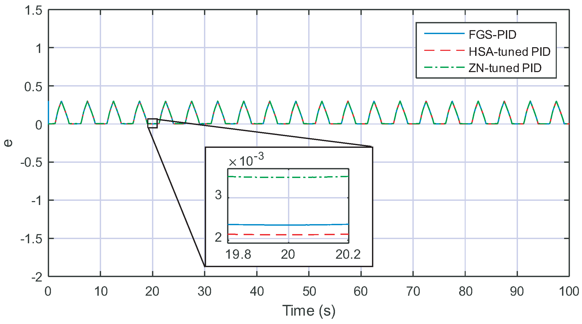
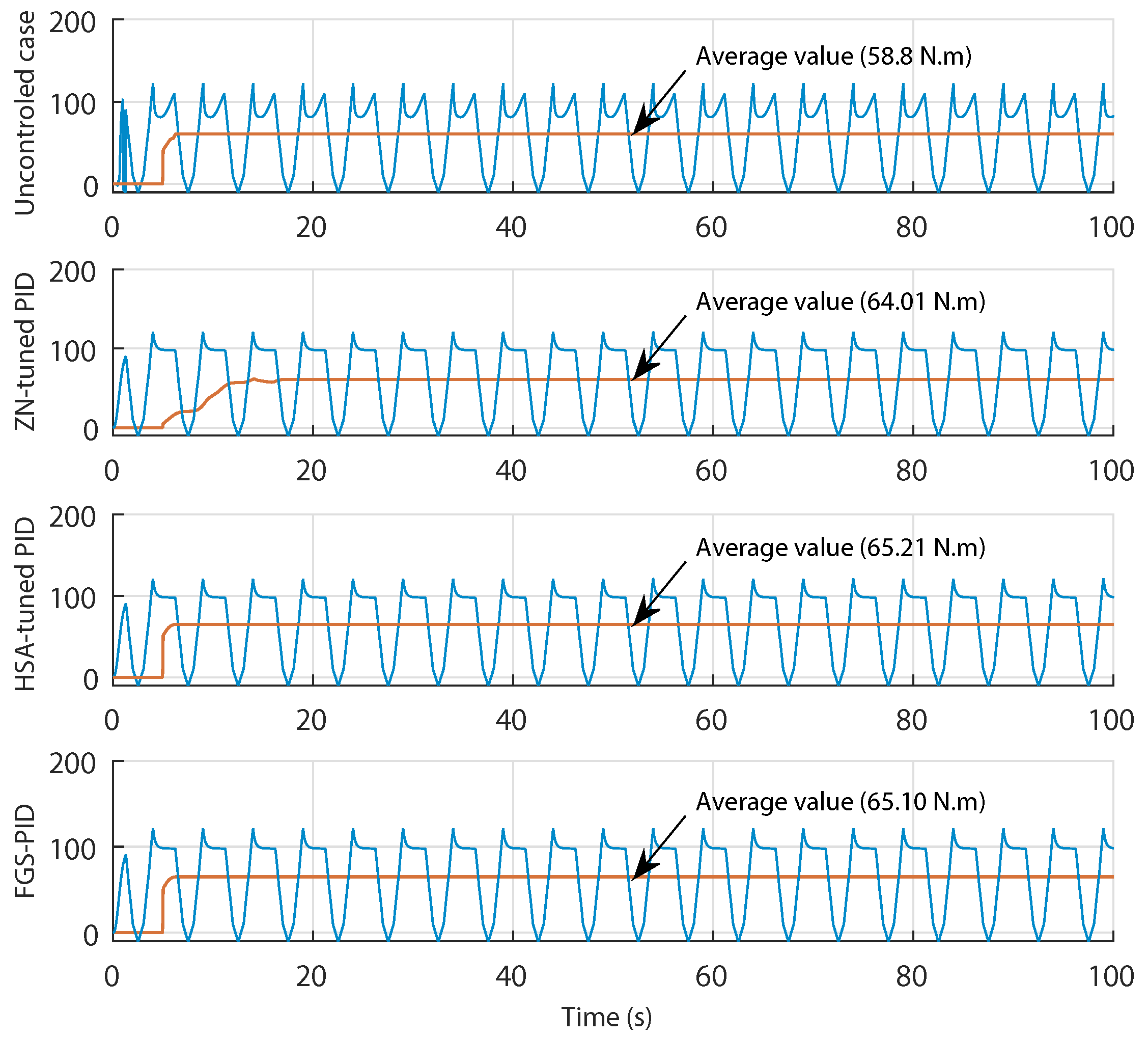
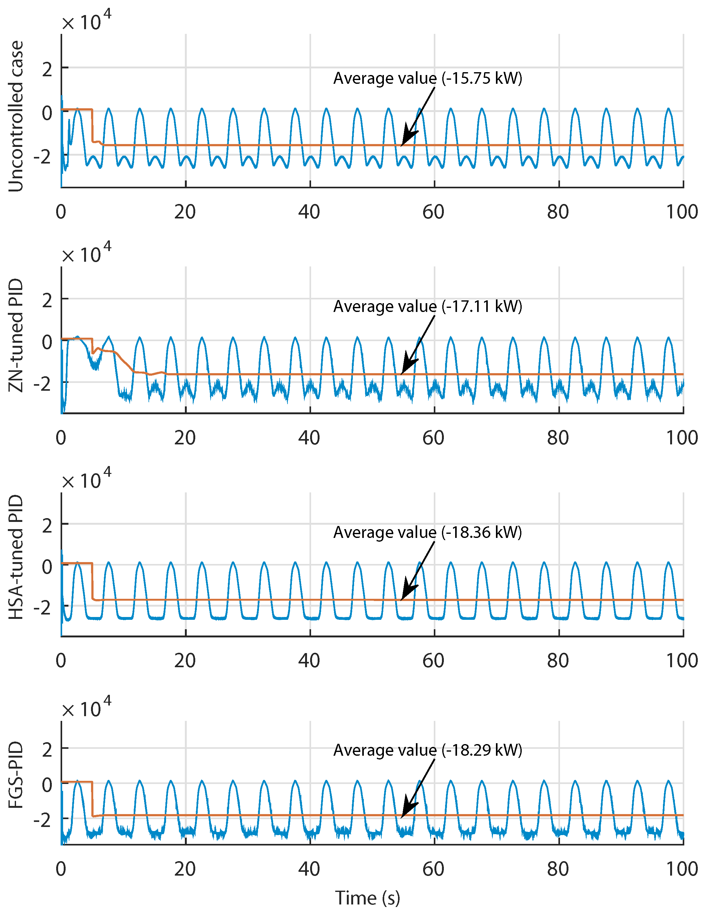
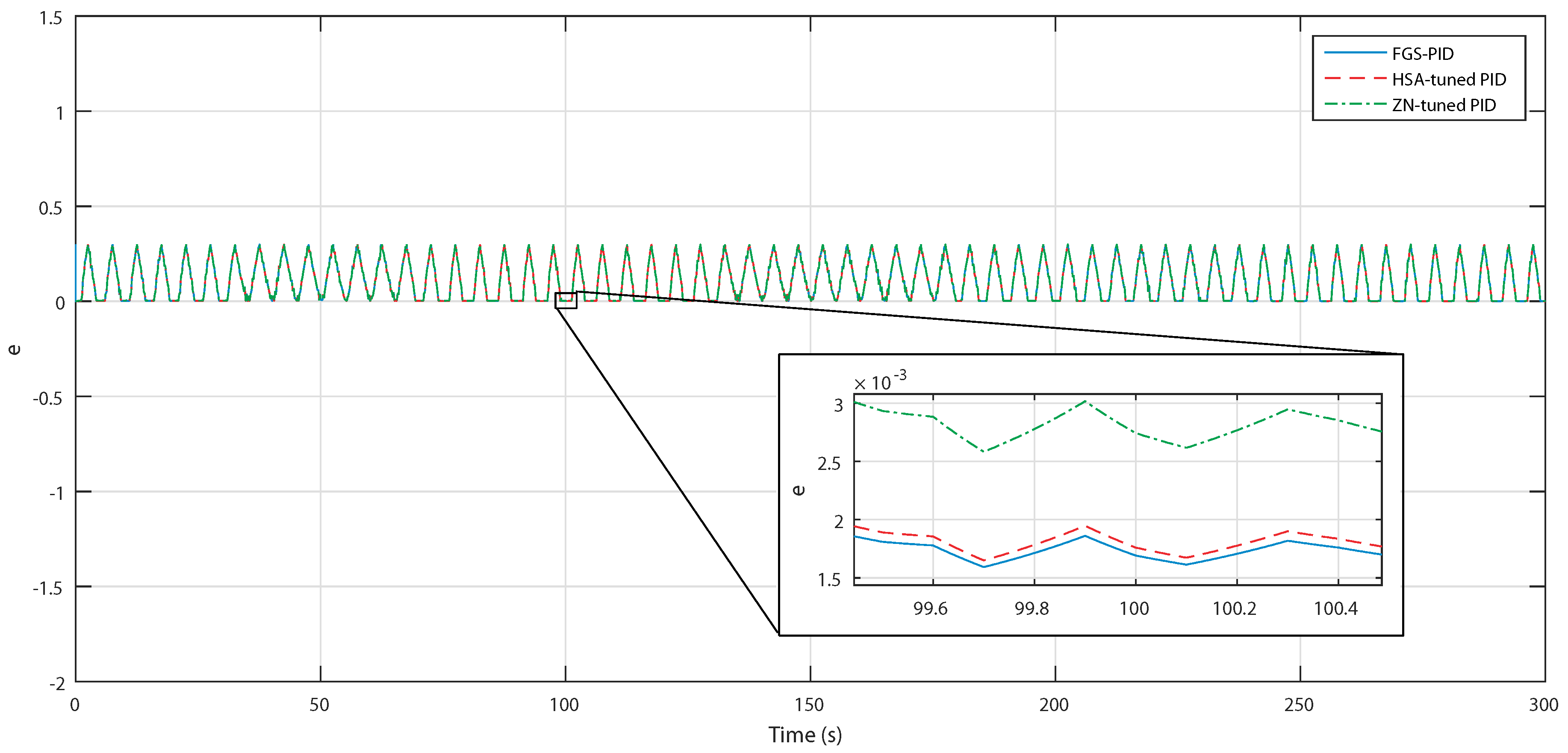
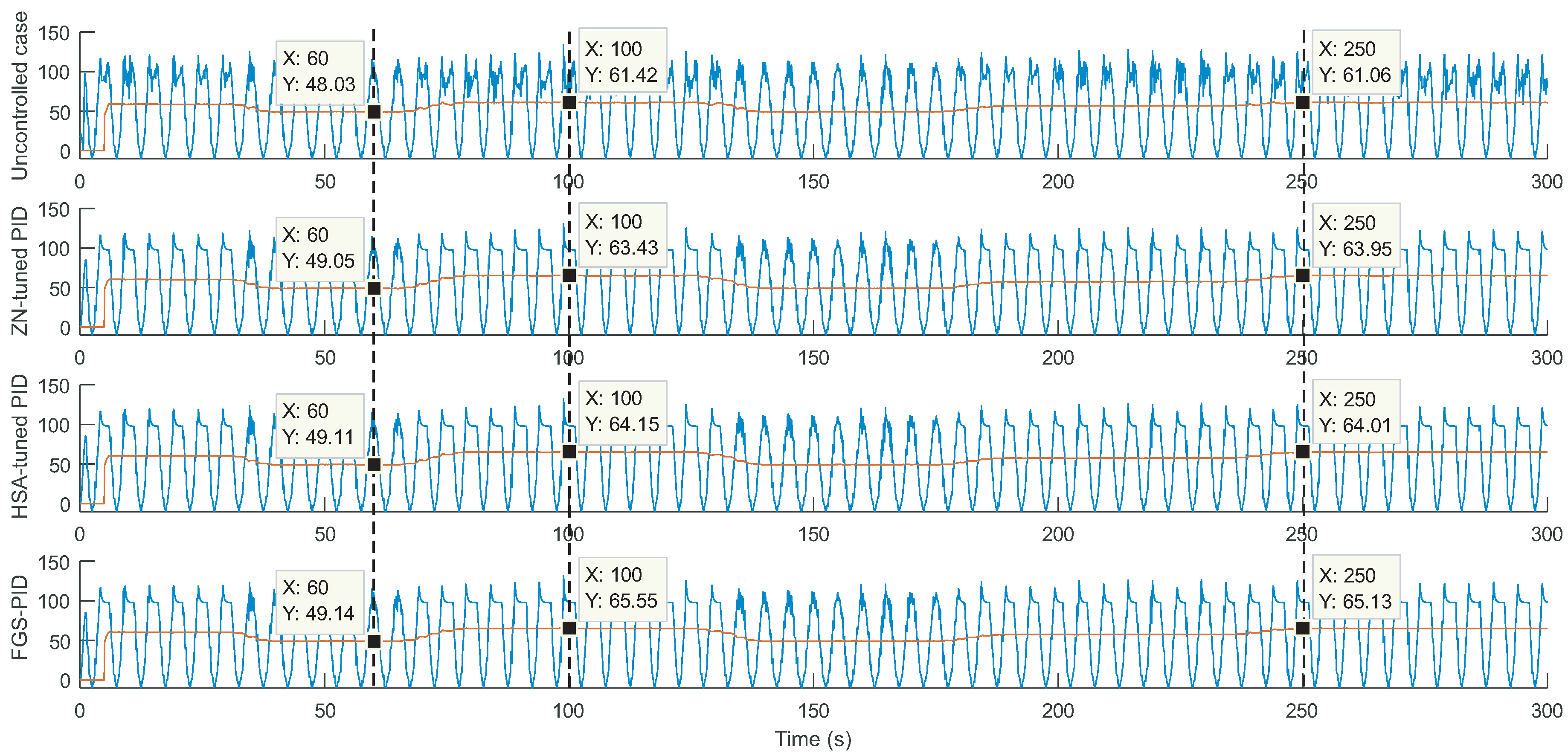
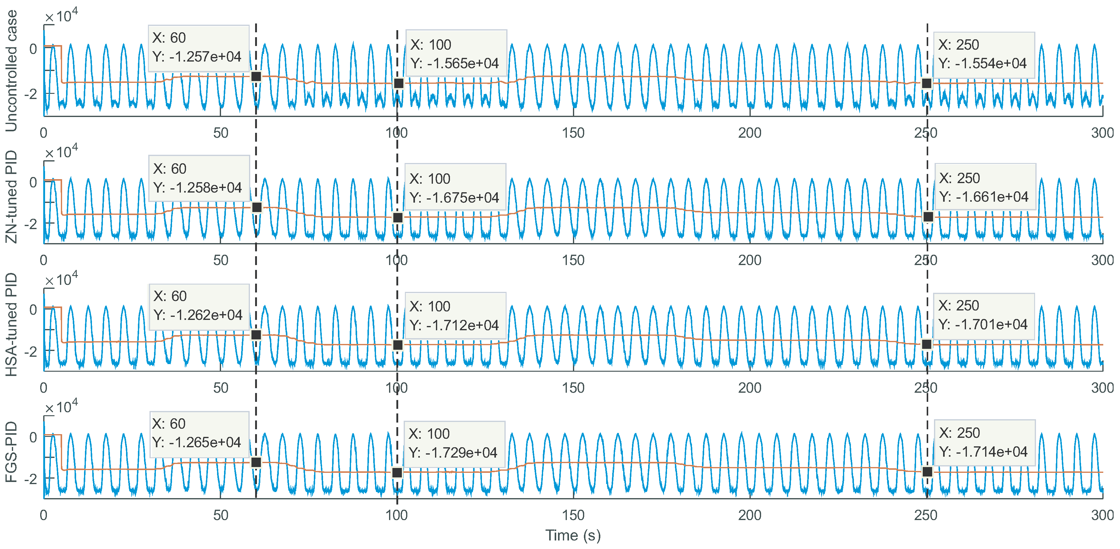
6.2. Performance in Regular Waves

To evaluate the power generation enhancement accomplished when using the suggested control design methodologies in regular waves, a study case was set up considering a representative sea state characterized by a wave period T w = 10 s, water depth h = 5 m, and a wave amplitude of A = 1.25 m. This input sea condition is considered to provoke the stalling behavior in the Wells turbine.
An investigation has been performed to compare the HSA-tuned PID and FGS-PID to a conventionally-tuned PID and to the uncontrolled case. In this context, Figure 17 shows all four flow coefficient of the OWC system in regular waves.
It can be seen from the zoom-in section of the plot in Figure 17 that all controlled cases provided a flow coefficient close to the threshold value 0.3, unlike the uncontrolled case, which gave a flow coefficient that greatly exceeded the threshold value 0.3. However, the HSA offered the best adjustment with the closest value to 0.3, but did not exceed it, followed by the FGS technique. The ZN technique was sufficiently good, but slightly exceeded the threshold value.
The obtained flow coefficients may be explained by the error signal illustrated in Figure 18, which shows that when the waves were high, the controllers were regulating the the airflow and the error was reduced. The superiority of both proposed soft computing control design methodologies against the conventional ZN method can be observed from the zoom-in section of the figure.
Resulting from the obtained flow coefficient is the produced turbine torque shown in Figure 19, which shows the torque of the uncontrolled case affected by the stalling behavior, which decreased its average value to 58.8 N·m. On the other hand, all controlled cases avoided the stalling behavior, increasing the average value of the produced torques. It can be seen that the highest produced torque was obtained with the HSA tuning method with 65.21 N·m, followed by the FGS tuning with 65.10 N·m, and the traditionally-tuned PID with 64.01 N·m.
The generated power from the OWC in all four cases is shown in Figure 20.
Because the uncontrolled case was affected by the stalling phenomenon, the generated power was limited and low with an average value of −15.75 kW; whereas, all controlled cases had higher power generation thanks to the implemented airflow control. It can be seen that the highest generated power was obtained with the HSA tuning method with −18.36 kW, followed by the FGS tuning with −18.29 kW, and the traditionally-tuned PID with −17.11 kW.
The results of the study showed that airflow control successfully avoided the stalling phenomenon of the Wells turbine. Moreover, the proposed IC showed a superior performance against the conventional method. In fact, the HSA-tuned PID offered 16.57% power generation in regular waves, and the FGS-PID offered 16.12% power generation improvement; whereas, the conventionally-tuned PID offered only 8.63% generation improvement.

6.3. Performance in Irregular Waves

The irregular wave model presented in Section 2 has been considered for power generation improvement tests. To make this model specific to the waves at the site of Mutriku, the wave characteristics from the representative wave spectrum were used. The significant wave height was H s = 2.44 m, and the mean wave period was T w = 10 s.
The flow coefficient of the OWC system in irregular waves using the different control design methodologies is presented in Figure 21. It can be seen in the uncontrolled case that the flow coefficient fluctuated and in some regions exceeded the threshold value 0.3. Using the proposed airflow control, it is shown that the flow coefficient was regulated to the desired value 0.3.
The error signal of all three controls are illustrated in Figure 22, which shows that when the waves were high enough, the controllers were regulating the the airflow, and the error was reduced. The superiority of the FGS-PID over the HSA-tuned PID and the ZN-tuned PID can be observed from the zoom-in section of the figure.
The produced turbine torque of the OWC system is illustrated in Figure 23. To compare the controlled cases to the uncontrolled case, three instances were considered at t 1 = 60 s, t 2 = 100 s, and t 3 = 250 s to measure the torque in terms of the average value. It can be seen in all three instances that the produced turbine torque with airflow control was higher than that of the uncontrolled case. Moreover, the average value of the torque obtained with the FGS-PID was the highest.
The resulting generated power was higher in the controlled cases than in the uncontrolled case, with the superiority of the FGS-PID. In Figure 24, we can notice that the average value of the generated power, in all three instances, t 1 , t 2 , and t 3 , is higher when using FGS-PID followed by the HSA-tuned PID.
The superiority of the FGS-PID over the HSA-tune PID in irregular waves is due to the fact that the gains of the controller were computed in real time using the fuzzy supervisor. This allows the gains of the FGS-PID to vary according to the changes in the varying inputs. On the other hand, the HSA-tuned PID had the optimal gains, but could not adapt to the changes as well as the FGS-PID.
With conventional tuning methods, the PID controller was tuned on a pre-specified operating point and without any direct knowledge of the system to be controlled. These characteristics limit the performance of the PID. The use of optimization algorithms such as the HSA helped overcome this limitation and improved the controller performance in regular waves. However, when the operating state of the power system varied with the irregular waves, the PID controller could not offer the assigned desirable performance. The optimum performance was achieved if the PID controller was capable of continuously tracking the changes occurring in the power system. This was achieved by the fuzzy gain scheduling, an intelligent approach for online tuning. In fact, the FGS-PID offered 6.77% power generation improvement in irregular waves followed by the HSA-tuned PID with 5.29%; whereas, the conventionally-tuned PID offered only 4.39% power generation improvement.

7. Conclusions

In this article, the NEREIDA OWC-based wave power plant has been modeled and controlled. The airflow control strategy was implemented to deal with the stalling phenomenon, which is a feature of the Wells turbine that limits the generated power. The airflow strategy effectively controls the throttle valve to adjust the airflow in the turbine duct and thus avoid the stalling phenomenon.
To improve the performance of the PID controller, two intelligent control design methodologies were proposed and implemented. The first approach is based on advanced metaheuristic algorithms, which allowed us to compute the optimal gains of the controller. The harmony search algorithm has been considered and compared to other advanced algorithms, and it provided interesting results. The second method was based on a novel fuzzy gain-scheduled PID controller, which adaptively changes the controller’s gains using the designed fuzzy supervisors in real time.
To test the effectiveness of the proposed controls, two sea conditions of regular and irregular waves have been considered for the investigation. The waves were chosen from the site of Mutriku in order to provoke the stalling behavior of the Wells turbine. The results obtained prove that proposed intelligent controls not only successfully avoid the stalling behavior, enabling the plant to extract the full power of the incoming waves, but also provides better performance and higher power generation improvement than those of the airflow control using a conventional PID controller.

Author Contributions

All authors contributed to the modeling and implementation of this work. F.M. conceived of, developed, and implemented the control techniques. All authors analyzed and validated the results. All authors contributed to the writing, review and editing of the manuscript.

Funding

This work was supported in part by the University of the Basque Country (UPV/EHU) through Project PPG17/33 and by MINECO through the Research Project DPI2015-70075-R (MINECO/FEDER, EU).

Acknowledgments

The authors would like to thank the editor and reviewers for the constructive comments that have helped to improve this paper.

Conflicts of Interest

The authors declare no conflict of interest.

References

  1. Alamir, M.; Fiacchini, M.; Chabane, S.B.; Bacha, S.; Kovaltchouk, T. Active power control under Grid Code constraints for a tidal farm. In Proceedings of the 2016 Eleventh International Conference on Ecological Vehicles and Renewable Energies (EVER), Monte Carlo, Monaco, 6–8 April 2016; pp. 1–7. [Google Scholar]
  2. Magagna, D.; Uihlein, A. 2014 JRC Ocean Energy Status Report; European Commission: Luxembourg, 2015. [Google Scholar]
  3. Stopa, J.E.; Cheung, K.F.; Chen, Y.L. Assessment of wave energy resources in Hawaii. Renew. Energy 2011, 36, 554–567. [Google Scholar] [CrossRef]
  4. Liberti, L.; Carillo, A.; Sannino, G. Wave energy resource assessment in the Mediterranean, the Italian perspective. Renew. Energy 2011, 50, 938–949. [Google Scholar] [CrossRef]
  5. Kumar, V.S.; Anoop, T.R. Wave energy resource assessment for the Indian shelf seas. Renew. Energy 2015, 76, 212–219. [Google Scholar] [CrossRef]
  6. Lopez, M.; Veigas, M.; Iglesias, G. On the wave energy resource of Peru. Energy Convers. Manag. 2015, 90, 34–40. [Google Scholar] [CrossRef]
  7. Scottish Energy Association. Available online: http://www.wearesea.com/ (accessed on 7 October 2018).
  8. Falcão, A.F.O.; Rodrigues, R.J.A. Stochastic modeling of OWC wave power plant performance. Appl. Ocean Res. 2002, 24, 59–71. [Google Scholar] [CrossRef]
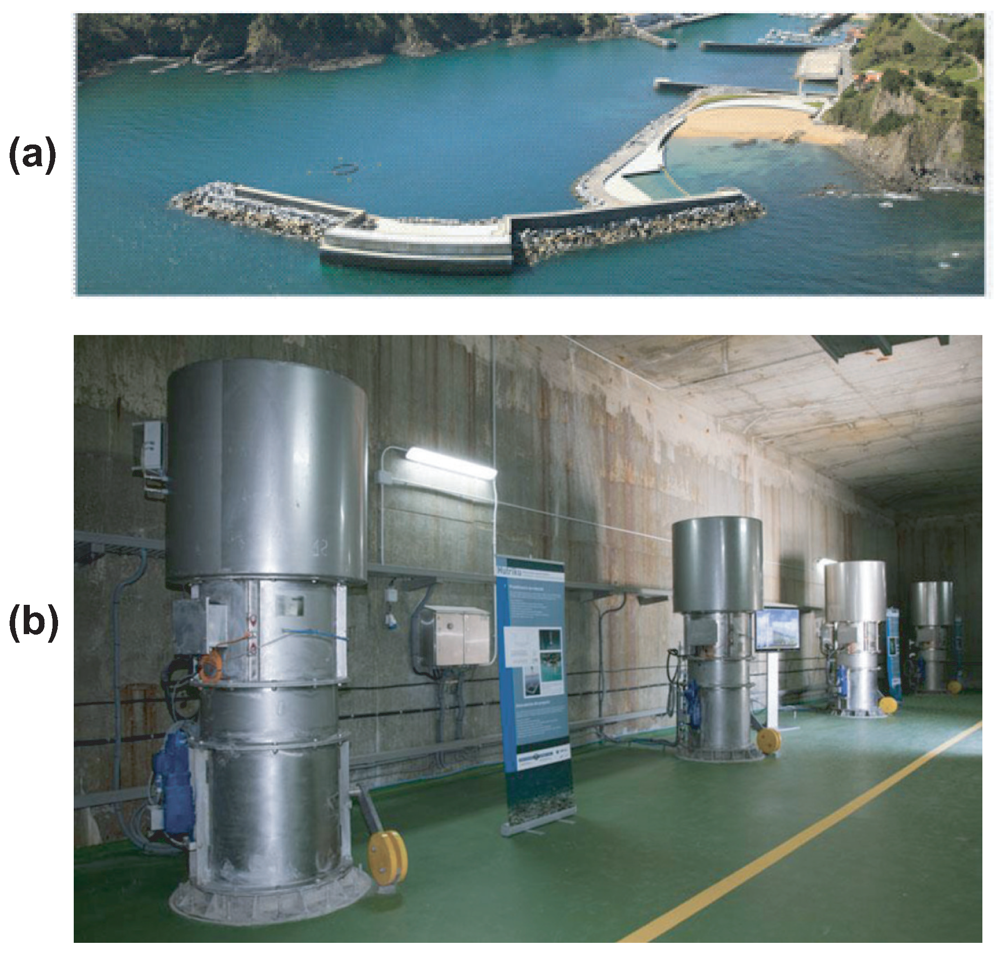
  9. Torre-Enciso, Y.; Ortubia, I.; López de Aguileta, L.I.; Marqués, J. Mutriku Wave Power Plant: From the thinking out to the reality. In Proceedings of the 8th European Wave and Tidal Energy Conference, Uppsala, Sweden, 7–10 September 2009; pp. 319–329. [Google Scholar]
  10. Tease, W.K.; Lees, J.; Hall, A. Advances in oscillating water column air turbine development. In Proceedings of the 7th European Wave and Tidal Energy Conference, Porto, Portugal, 11–14 September 2007. [Google Scholar]
  11. Raghunathan, S. Performance of the Wells self-rectifying turbine. Aeronaut. J. 1985, 89, 369–379. [Google Scholar]
  12. Raghunathan, S. The wells air turbine for wave energy conversion. Prog. Aerosp. Sci. 1995, 31, 335–386. [Google Scholar] [CrossRef]
  13. M’zoughi, F.; Bouallègue, S.; Ayadi, M. Modeling and SIL simulation of an oscillating water column for ocean energy conversion. In Proceedings of the 2015 6th International Renewable Energy Congress (IREC), Sousse, Tunisia, 24–26 March 2015; pp. 1–6. [Google Scholar]
  14. M’zoughi, F.; Bouallègue, S.; Ayadi, M.; Garrido, A.J.; Garrido, I. Modeling and airflow control of an oscillating water column for wave power generation. In Proceedings of the 2017 4th International Conference on Control, Decision and Information Technologies (CoDIT), Barcelona, Spain, 5–7 April 2017; pp. 938–943. [Google Scholar]
  15. Sobey, R.; Goodwin, P.; Thieke, R.; Westberg, R.J., Jr. Application of Stokes, Cnoidal, and Fourier wave theories. J. Waterw. Port Coast. Ocean Eng. 1987, 113, 565–587. [Google Scholar] [CrossRef]
  16. Tromans, P.S.; Anaturk, A.R.; Hagemeijer, P. A new model for the kinematics of large ocean waves-application as a design wave. In Proceedings of the First International Offshore and Polar Engineering Conference, Edinburgh, UK, 11–16 August 1991. [Google Scholar]
  17. Chadwick, A.; Morfett, J.; Borthwick, M. Hydraulics in Civil and Environmental Engineering; Spon Press: London, UK, 2004. [Google Scholar]
  18. Garrido, A.J.; Otaola, E.; Garrido, I.; Lekube, J.; Maseda, F.J.; Liria, P.; Mader, J. Mathematical Modeling of Oscillating Water Columns Wave-Structure Interaction in Ocean Energy Plants. Math. Probl. Eng. 2015, 2015, 727982. [Google Scholar] [CrossRef]
  19. Le Roux, J.P. An extension of the Airy theory for linear waves into shallow water. Coast. Eng. 2008, 55, 295–301. [Google Scholar] [CrossRef]
  20. Sarmento, A.J.N.A.; Falcão, A.F.D.O. Wave generation by an oscillating surface-pressure and its application in wave-energy extraction. J. Fluid Mech. 1985, 150, 467–485. [Google Scholar] [CrossRef]
  21. Falcao, A.F.D.O.; Justino, P.A.P. OWC wave energy devices with air flow control. Ocean Eng. 1999, 26, 1275–1295. [Google Scholar] [CrossRef]
  22. M’zoughi, F.; Bouallègue, S.; Garrido, A.J.; Garrido, I.; Ayadi, M. Stalling-free Control Strategies for Oscillating-Water-Column-based Wave Power Generation Plants. IEEE Trans. Energy Convers. 2018, 33, 209–222. [Google Scholar] [CrossRef]
  23. M’zoughi, F.; Bouallègue, S.; Garrido, A.J.; Garrido, I.; Ayadi, M. Water Cycle Algorithm-based Airflow Control for an Oscillating Water Column-based Wave Generation Power Plant. Proc. Inst. Mech. Eng. Part I J. Syst. Control Eng. 2018, 2018. [Google Scholar] [CrossRef]
  24. Lekube, J.; Garrido, A.J.; Garrido, I.; Otaola, E. Output Power Improvement in Oscillating Water Column-based Wave Power Plants. Revista Iberoamericana de Automática e Informática Industrial 2018, 15, 145–155. [Google Scholar] [CrossRef]
  25. Falcão, A.F.O.; Gato, L.M.C. Air Turbines. In Comprehensive Renewable Energy; Sayigh, A., Ed.; 8: Ocean Energy; Elsevier: Oxford, UK, 2012; pp. 111–149. [Google Scholar] [CrossRef]
  26. López, I.; Andreu, J.; Ceballos, S.; de Alegría, I.M.; Kortabarria, I. Review of wave energy technologies and the necessary power-equipment. Renew. Sustain. Energy Rev. 2013, 27, 413–434. [Google Scholar] [CrossRef]
  27. Setoguchi, T.; Takao, M. Current status of self rectifying air turbines for wave energy conversion. Energy Convers. Manag. 2006, 47, 2382–2396. [Google Scholar] [CrossRef]
  28. O’Sullivan, D.L.; Lewis, A. Generator selection and comparative performance in offshore oscillating water column. IEEE Trans. Energy Convers. 2011, 26, 603–614. [Google Scholar] [CrossRef]
  29. Alberdi, M.; Amundarain, M.; Garrido, A.J.; Garrido, I.; Casquero, O.; De la Sen, M. Complementary control of oscillating water column-based wave energy conversion plants to improve the instantaneous power output. IEEE Trans. Energy Convers. 2011, 26, 1021–1032. [Google Scholar] [CrossRef]
  30. Muller, S.; Diecke, M.; De Donker, R.W. Doubly fed induction generator systems for wind turbines. IEEE Ind. Appl. Mag. 2002, 8, 26–33. [Google Scholar] [CrossRef]
  31. Ledesma, P.; Usaola, J. Doubly fed induction generator model for transient stability analysis. IEEE Trans. Energy Convers. 2005, 20, 388–397. [Google Scholar] [CrossRef]
  32. M’zoughi, F.; Garrido, A.J.; Garrido, I.; Bouallègue, S.; Ayadi, M. Sliding Mode Rotational Speed Control of an Oscillating Water Column-based Wave Generation Power Plants. In Proceedings of the 2018 International Symposium on Power Electronics, Electrical Drives, Automation and Motion (SPEEDAM), Amalfi, Italy, 20–22 June 2018; pp. 1263–1270. [Google Scholar]
  33. Amundarain, M.; Alberdi, M.; Garrido, A.J.; Garrido, I. Modeling and simulation of wave energy generation plants: Output power control. IEEE Trans. Ind. Electron. 2011, 58, 105–117. [Google Scholar] [CrossRef]
  34. Chen, Z.; Guerrero, J.M.; Blaabjerg, F. A review of the state of the art of power electronics for wind turbines. IEEE Trans. Power Electron. 2009, 24, 1859–1875. [Google Scholar] [CrossRef]
  35. Fletcher, J.; Yang, J. Introduction to the Doubly-Fed Induction Generator for Wind Power Applications. In Paths to Sustainable Energy; INTECH Open Access Publisher: London, UK, 2010. [Google Scholar] [Green Version]
  36. Lei, Y.; Mullane, A.; Lightbody, G.; Yacamini, R. Modeling of the wind turbine with a doubly fed induction generator for grid integration studies. IEEE Trans. Energy Convers. 2006, 21, 257–264. [Google Scholar] [CrossRef]
  37. Bouallègue, S.; Haggège, J.; Benrejeb, M. A new method for tuning PID-type fuzzy controllers using particle swarm optimization. In Fuzzy Controllers-Recent Advances in Theory and Applications; InTech.: London, UK, 2012. [Google Scholar]
  38. Bouallègue, S.; Haggège, J.; Ayadi, M.; Benrejeb, M. PID-type fuzzy logic controller tuning based on particle swarm optimization. Eng. Appl. Artif. Intell. 2012, 25, 484–493. [Google Scholar] [CrossRef]
  39. Eberhart, R.C.; Kennedy, J. A new optimizer using particle swarm theory. In Proceedings of the 6th International Symposium on micro Machine and Human Science MHS’95, Nagoya, Japan, 4–6 October 1995; pp. 39–43. [Google Scholar]
  40. Legowski, A.; Niezabitowski, M. Robot path control based on PSO with fractional-order velocity. In Proceedings of the International Conference on Robotics and Automation Engineering (ICRAE), Jeju Island, Korea, 27–29 August 2016; pp. 21–25. [Google Scholar]
  41. Zotes, F.A.; Santos Penas, M. Heuristic Optimization of Interplanetary Trajectories in Aerospace Missions. Revista Iberoamericana de Automatica e Informatica Industrial 2017, 14, 1–15. [Google Scholar] [CrossRef]
  42. Clerc, M.; Kennedy, J. The Particle Swarm-Explosion, Stability, and Convergence in a Multidimensional Complex Space. IEEE Trans. Evolut. Comput. 2002, 6, 58–73. [Google Scholar] [CrossRef]
  43. Bouallègue, S.; Haggège, J.; Benrejeb, M. Particle Swarm Optimization-Based Fixed-Structure H Control Design. Int. J. Control Autom. Syst. 2011, 9, 258–266. [Google Scholar] [CrossRef]
  44. Eskandar, H.; Sadollah, A.; Bahreininejad, A.; Hamdi, M. Water cycle algorithm—A novel metaheuristic optimization method for solving constrained engineering optimization problems. Comput. Struct. 2012, 30, 151–166. [Google Scholar] [CrossRef]
  45. Pahnehkolaei, S.M.A.; Alfi, A.; Sadollah, A.; Kim, J.H. Gradient-based Water Cycle Algorithm with evaporation rate applied to chaos suppression. Appl. Soft Comput. 2017, 30, 420–440. [Google Scholar] [CrossRef]
  46. Geem, Z.W.; Kim, J.H.; Loganathan, G.V. A new heuristic optimization algorithm: Harmony search. Simulation 2001, 76, 60–68. [Google Scholar] [CrossRef]
  47. Wang, X.; Gao, X.Z.; Zenger, K. An Introduction to Harmony Search Optimization Method; Springer International Publishing: Cham, Switzerland, 2015. [Google Scholar]
  48. Gao, X.Z.; Govindasamy, V.; Xu, H.; Wang, X.; Zenger, K. Harmony search method: Theory and applications. Comput. Intel. Neurosci. 2015, 2015, 39–48. [Google Scholar] [CrossRef]
  49. M’zoughi, F.; Bouallègue, S.; Ayadi, M.; Garrido, A.J.; Garrido, I. Harmony Search Algorithm-based Airflow Control of an Oscillating Water Column-based Wave Generation Power Plants. In Proceedings of the 2018 International Conference on Advanced Systems and Electric Technologies (IC_ASET), Hammamet, Tunisia, 22–25 March 2018; pp. 249–254. [Google Scholar]
  50. Zaho, Z.Y.; Tomizuka, M.; Isaka, S. Fuzzy Gain Scheduling of PID Controllers. IEEE Trans. Syst. Man Cybern. 1993, 23, 1392–1398. [Google Scholar]
  51. Tursini, M.; Parasiliti, F.; Zhang, D. Real-time gain tuning of PI controllers for high-performance PMSM drives. IEEE Trans. Ind. Appl. 2002, 38, 1018–1026. [Google Scholar] [CrossRef]
  52. Dounis, A.I.; Kofinas, P.; Alafodimos, C.; Tseles, D. Adaptive fuzzy gain scheduling PID controller for maximum power point tracking of photovoltaic system. Renew. Energy 2013, 60, 202–214. [Google Scholar] [CrossRef]
  53. Bedoud, K.; Ali-rachedi, M.; Bahi, T.; Lakel, R. Adaptive fuzzy gain scheduling of PI controller for control of the wind energy conversion systems. Energy Procedia 2015, 74, 211–225. [Google Scholar] [CrossRef]
  54. Ziegler, J.G.; Nichols, N.B. Optimum settings for automatic controllers. Trans. ASME 1942, 64, 759–765. [Google Scholar] [CrossRef]
  55. Aström, K.J.; Hägglund, T. Advanced PID Control; ISA—The Instrumentation, Systems and Automation Society: Research Triangle Park, NC, USA, 2006. [Google Scholar]
  56. Hang, C.C.; Aström, K.J.; Ho, W.K. Refinements of the Ziegler-Nichols tuning formula. IEE Proc. D Control Theory Appl. 1991, 138, 111–118. [Google Scholar] [CrossRef]
  57. Wang, Q.G.; Lee, T.H.; Fung, H.W.; Bi, Q.; Zhang, Y. PID tuning for improved performance. IEEE Trans. Control Syst. Technol. 1999, 7, 457–465. [Google Scholar] [CrossRef]
Figure 1. NEREIDA wave power plant in Mutriku, Spain: (a) the plant and the breakwater; (b) PTO of OWC units inside the station.
Electronics 08 00070 g001
Figure 2. Scheme of the OWC station and the sea wave. SWL , Still Water Level.
Electronics 08 00070 g002
Figure 3. Representative spectral analysis of the waves at the site of Mutriku on 12 May 2014.
Electronics 08 00070 g003
Figure 4. Wells turbine of the NEREIDA OWC plant.
Electronics 08 00070 g004
Figure 5. Characteristic curves of the installed Wells turbine. (a) Power coefficient versus flow coefficient; (b) torque coefficient versus flow coefficient.
Electronics 08 00070 g005
Figure 6. Equivalent circuit of the DFIG in the d-axis.
Electronics 08 00070 g006
Figure 7. Equivalent circuit of the DFIG in the q-axis.
Electronics 08 00070 g007
Figure 8. Flow coefficient vs. time for two wave magnitudes [22,23].
Electronics 08 00070 g008
Figure 9. Turbine torques vs, time for two sea conditions [22,23].
Electronics 08 00070 g009
Figure 10. Airflow control scheme for a Wells turbine-based OWC wave power plant. GSC, Grid-Side Converter; RSC, Rotor-Side Converter.
Electronics 08 00070 g010
Figure 11. Advanced metaheuristic-based airflow control scheme for OWC.
Electronics 08 00070 g011
Figure 12. FGS-PID-based airflow control scheme for OWC.
Electronics 08 00070 g012
Figure 13. Membership functions for inputs e and Δ e . Negative Big (NB), Negative (N), Zero (Z), Positive (P), and Positive Big (PB).
Electronics 08 00070 g013
Figure 14. Membership functions for outputs K p , K i , and K d .
Electronics 08 00070 g014
Figure 15. Surface view of the fuzzy supervisor for K p , K i , and K d .
Electronics 08 00070 g015
Figure 16. Convergence curves of Problem (32).
Electronics 08 00070 g016
Figure 17. Flow coefficients with different control methodologies in regular waves. ZN, Ziegler–Nichols.
Electronics 08 00070 g017
Figure 18. Error signal with different control methodologies in regular waves.
Electronics 08 00070 g018
Figure 19. Turbine torque with different control methodologies in regular waves.
Electronics 08 00070 g019
Figure 20. Generated power with different control methodologies in regular waves.
Electronics 08 00070 g020
Figure 21. Flow coefficients with different control methodologies in irregular waves.
Electronics 08 00070 g021
Figure 22. Error signal with different control methodologies in irregular waves.
Electronics 08 00070 g022
Figure 23. Turbine torque with different control methodologies in irregular waves.
Electronics 08 00070 g023
Figure 24. Generated power with different control methodologies in irregular waves.
Electronics 08 00070 g024
Table 1. Fuzzy tuning rules for K p .
K p e k
NBNZPPB
NBNBNBNBNZ
NNBNNNZ
Δ e k ZNBNZPPB
PZPPPPB
PBZPPBPBPB
Table 2. Fuzzy tuning rules for K i .
K i e k
NBNZPPB
NBPBPBPBNNB
NPBPPZNB
Δ e k ZPPZNNB
PZPNNNB
PBZNNBNBNB
Table 3. Fuzzy tuning rules for K d .
K d e k
NBNZPPB
NBNBNBNBPPB
NNNNZPB
Δ e k ZZNZPPB
PZNPPPB
PBZPPBPBPB
Table 4. Plant parameters from the NEREIDA wave power plant at Mutriku.
Capture ChamberWells TurbineDFIG Generator
w c = 4.5 mn = 5 P r a t e d = 18.45 kW
l c = 4.3 mb = 0.21 m V s r a t e d = 400 V
ρ a = 1.19 kg/m 3 l = 0.165 m f r a t e d = 50 Hz
ρ w = 1029 kg/m 3 r = 0.375 m p = 2
a = 0.4417 m 2 R s = 0.5968 Ω
R r = 0.6258 Ω
L s s = 0.0003495 H
L r r = 0.324 H
L m = 0.324 H
Table 5. Results of the optimization from 20 trials of Problem (32): Particle Swarm Optimization with decreasing weight Inertia (PSO-In), the Fractional Particle Swarm Optimization Memetic Algorithm (FPSOMA), the Water Cycle Algorithm (WCA), and Harmony Search Algorithm (HSA).
AlgorithmBestMeanWorstS.D.
PSO-In8.0928.35711.7431.692
FPSOMA8.0018.3219.8641.468
WCA4.7126.8548.1311.586
HSA4.6385.5267.7281.331

