LiDAR and Camera Detection Fusion in a Real-Time Industrial Multi-Sensor Collision Avoidance System


Abstract
:1. Introduction
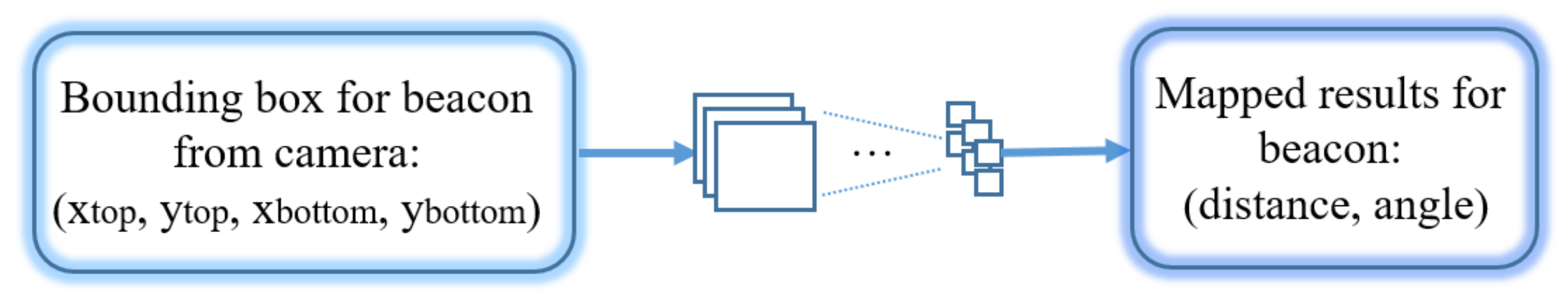
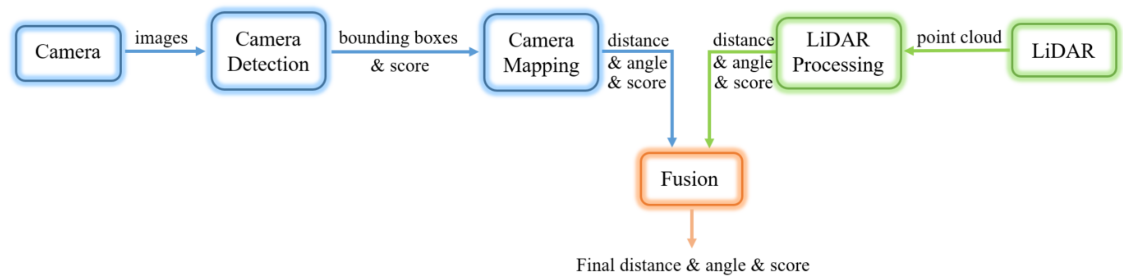
- We propose a fast and efficient method that learns the projection from the camera space to the LiDAR space and provides camera outputs in the form of LiDAR detection (distance and angle).
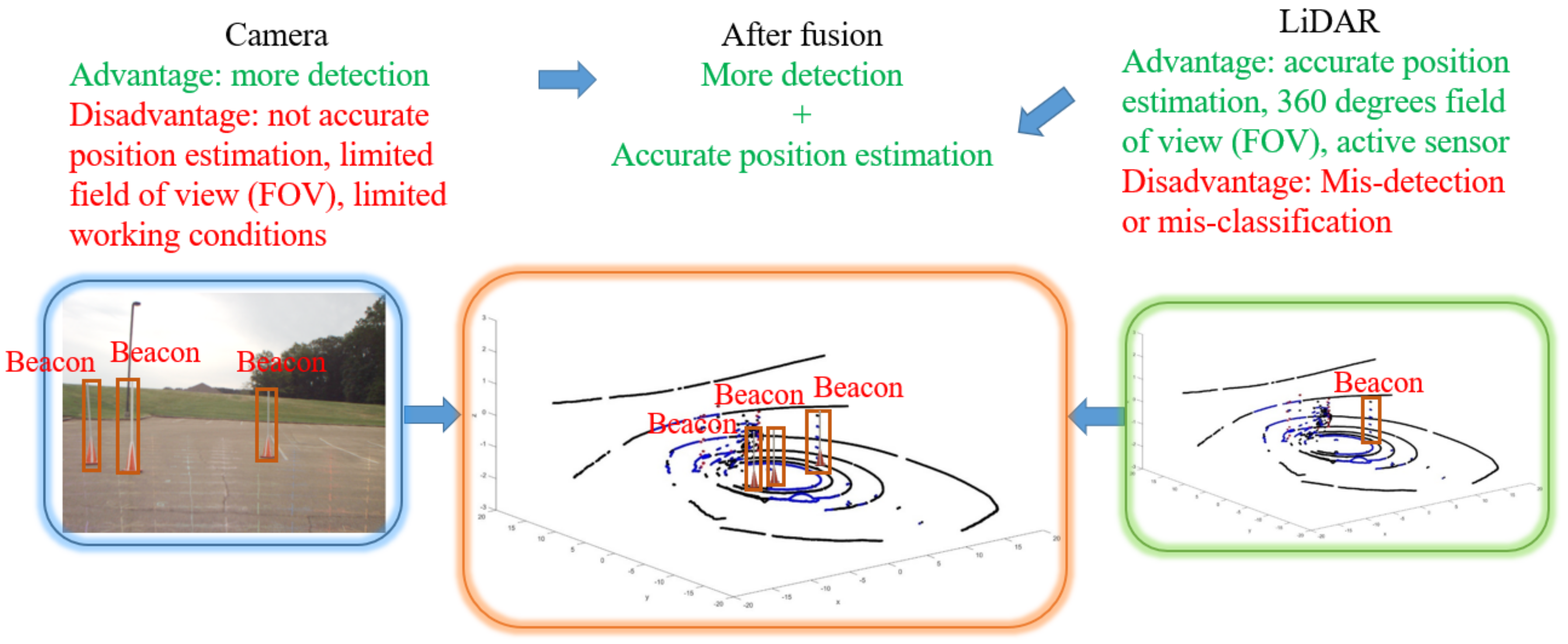
- We propose a multi-sensor detection system that fuses both the camera and LiDAR detections to obtain more accurate and robust beacon detections.
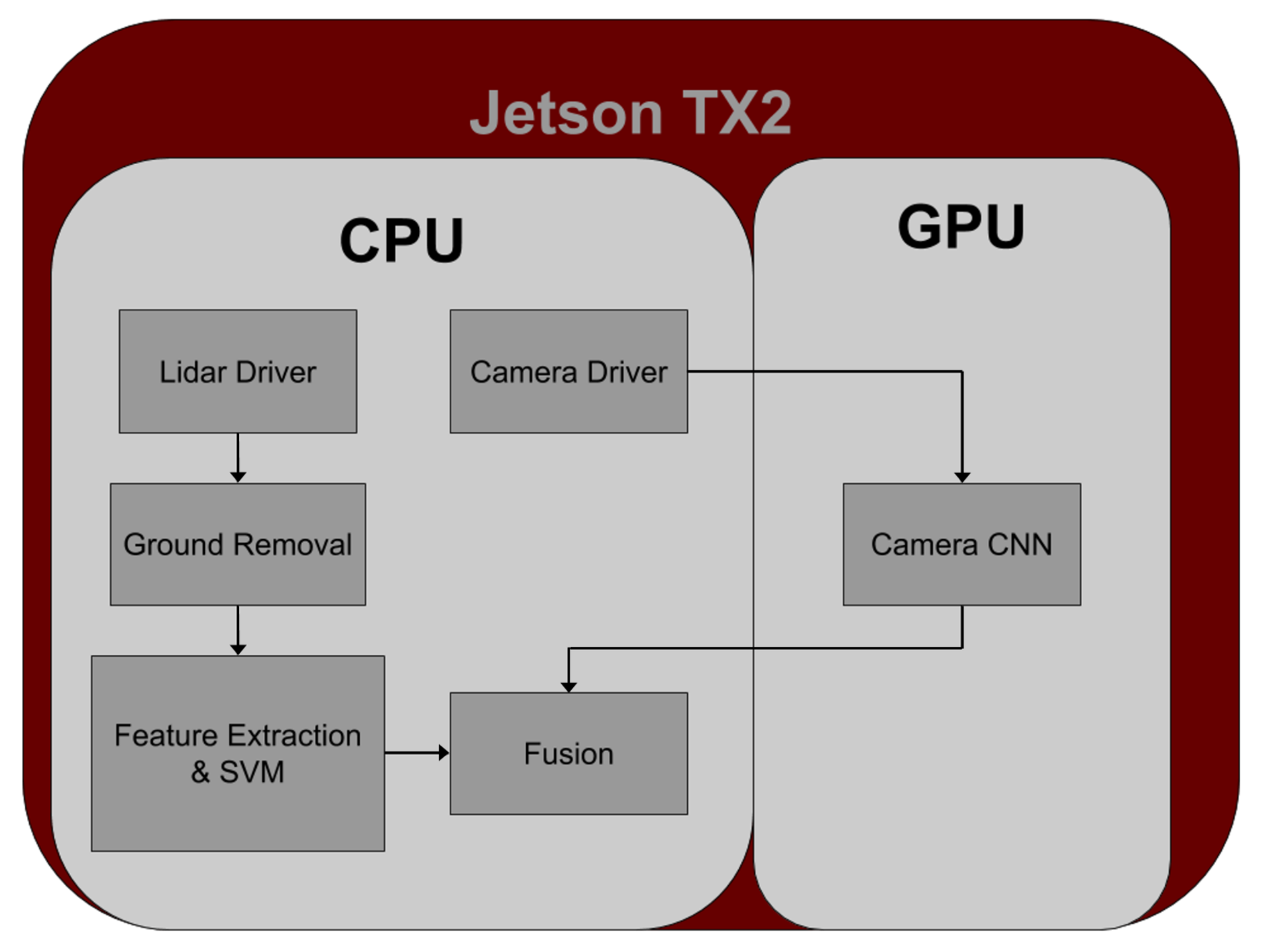
- The proposed solution has been implemented using a single Jetson TX2 board (dual CPUs and a GPU) board to run the sensor processing and a second TX2 for the model predictive control (MPC) system. The sensor processing runs in real time (5 Hz).
- The proposed fusion system has been built, integrated and tested using static and dynamic scenarios in a relevant environment. Experimental results are presented to show the fusion efficacy.
2. Background
2.1. Camera Detection
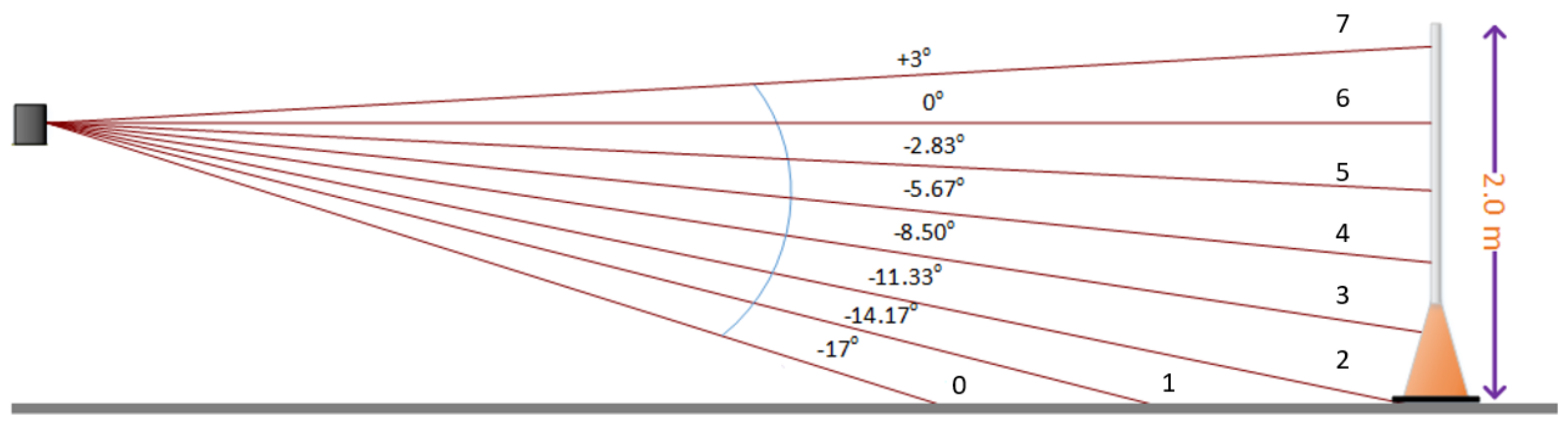
2.2. LiDAR Detection
2.3. Camera and LiDAR Detection Fusion
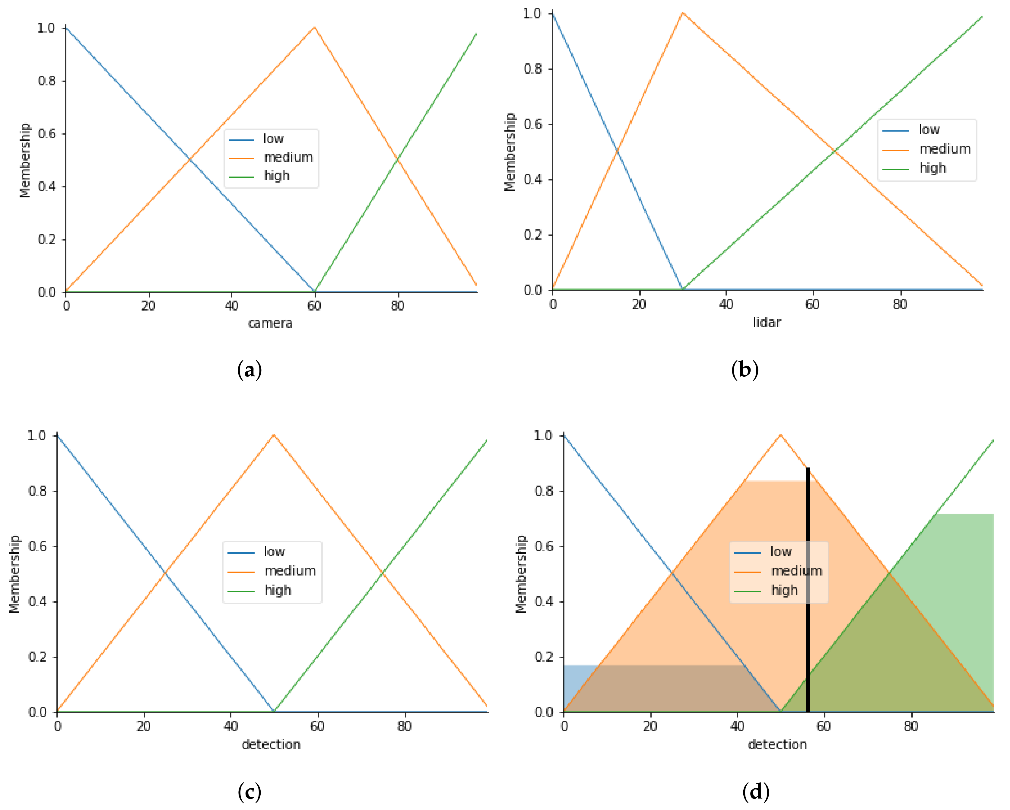
2.4. Fuzzy Logic
3. Proposed System
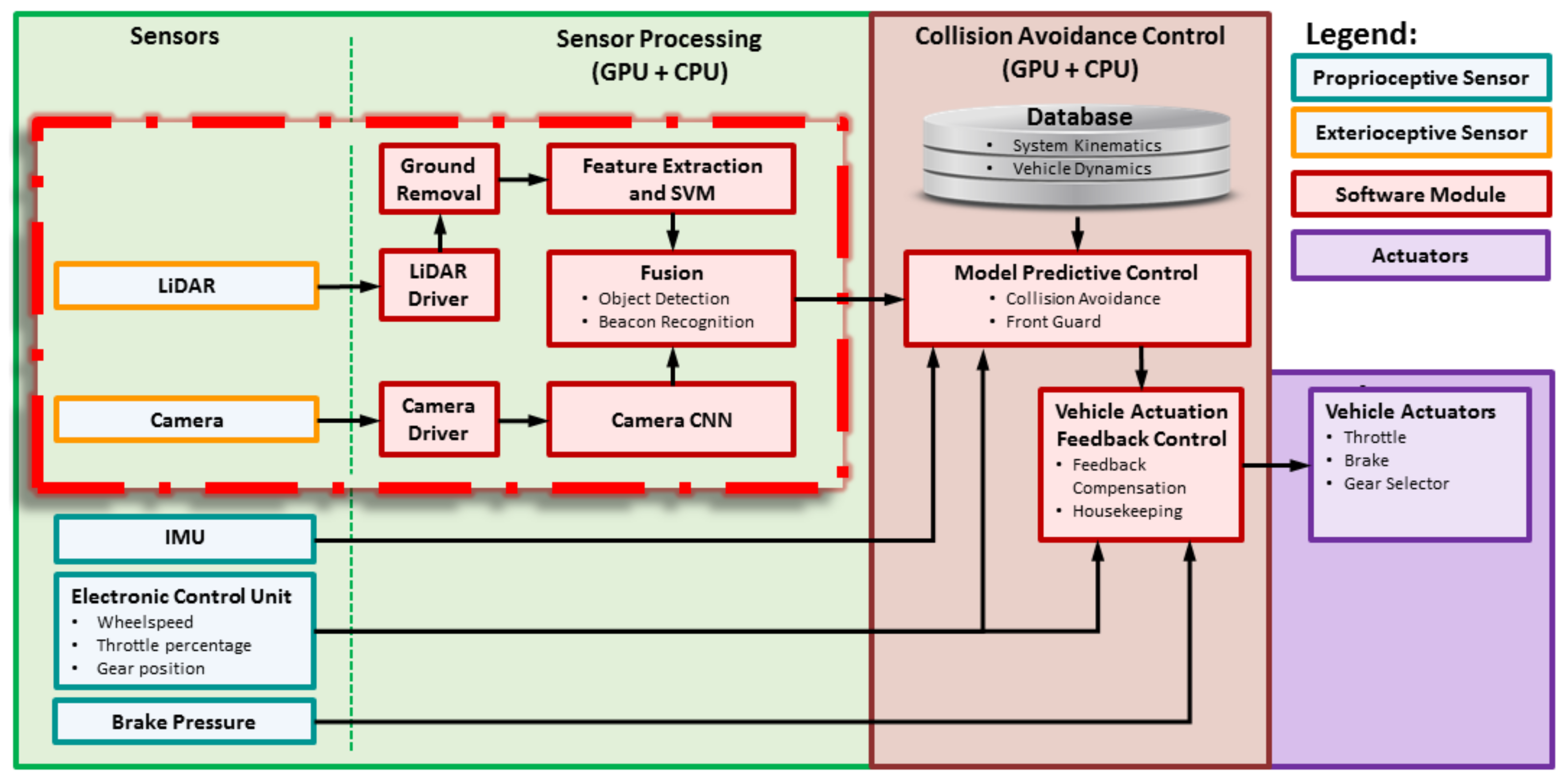
3.1. Overview
3.2. Real-Time Implementation
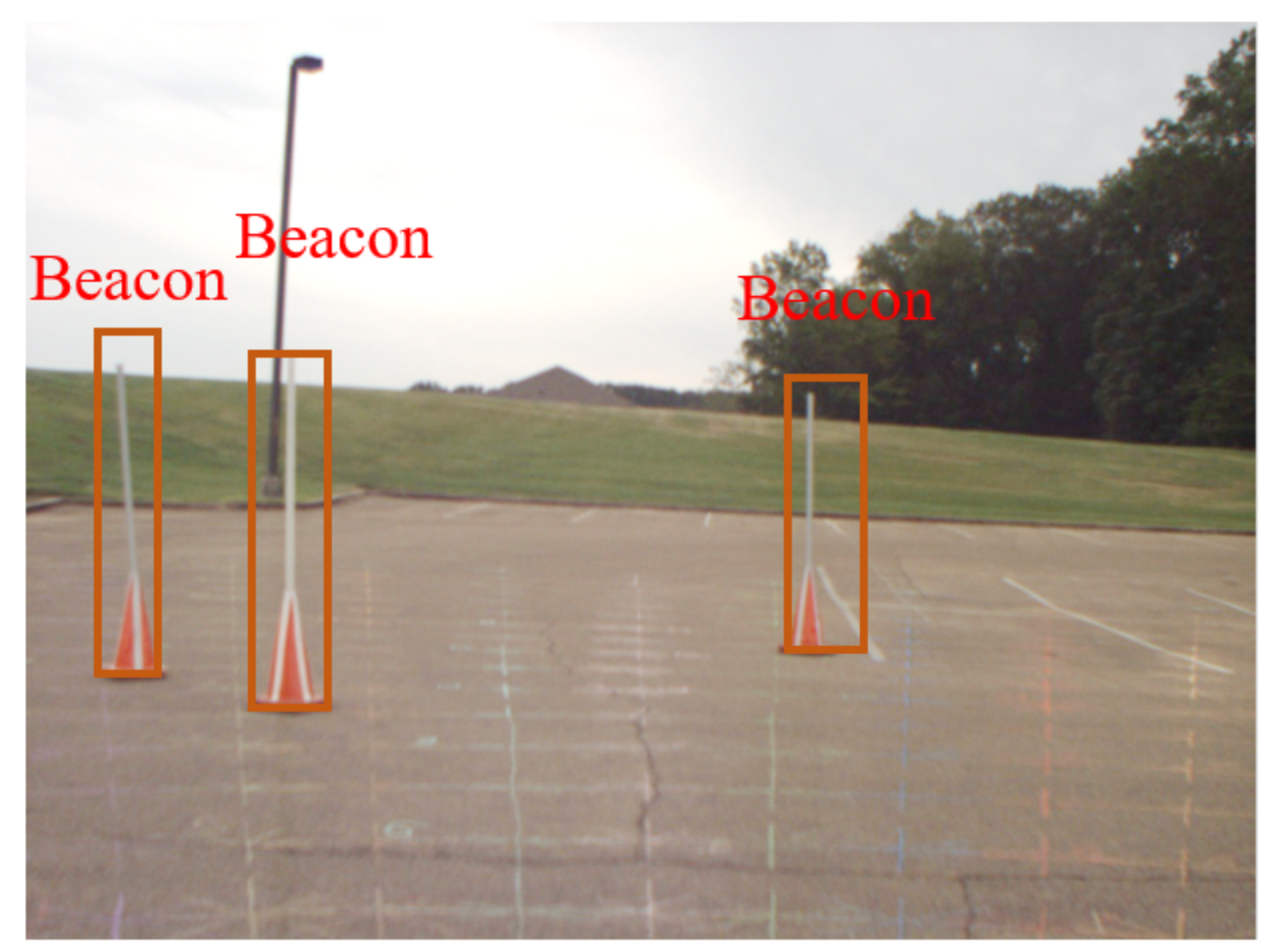
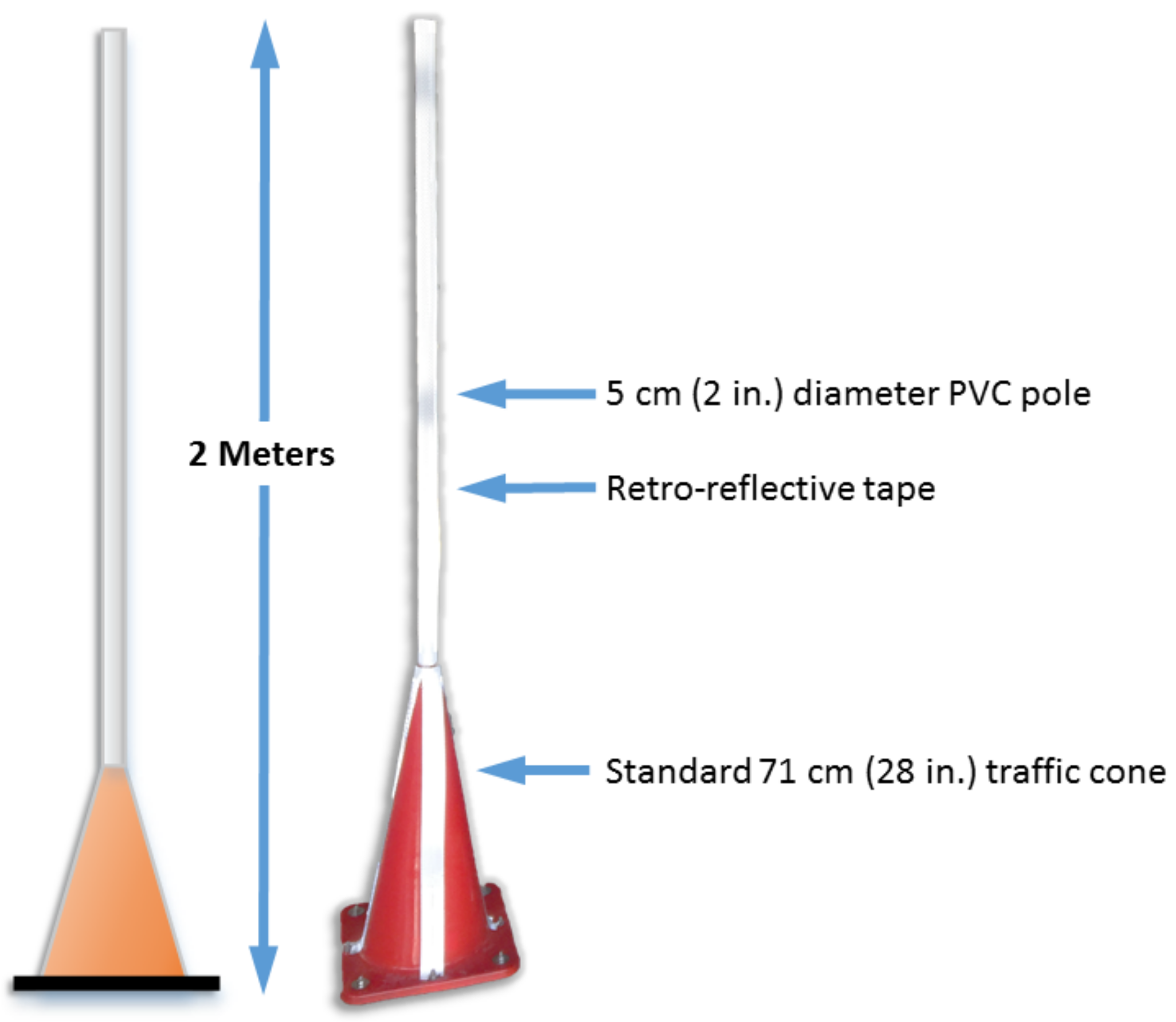
3.3. Beacon
3.4. Camera Detection
3.5. LiDAR Front Guard
3.6. LiDAR Beacon Detection
3.6.1. Overview
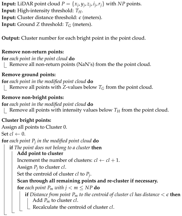
3.6.2. LiDAR Clustering
| Algorithm 1: LiDAR bright pixel clustering. |
 |
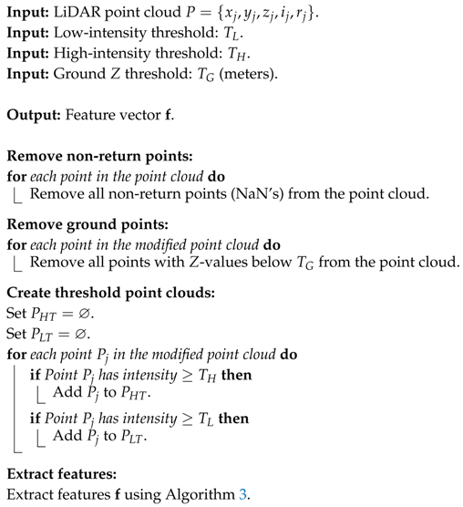
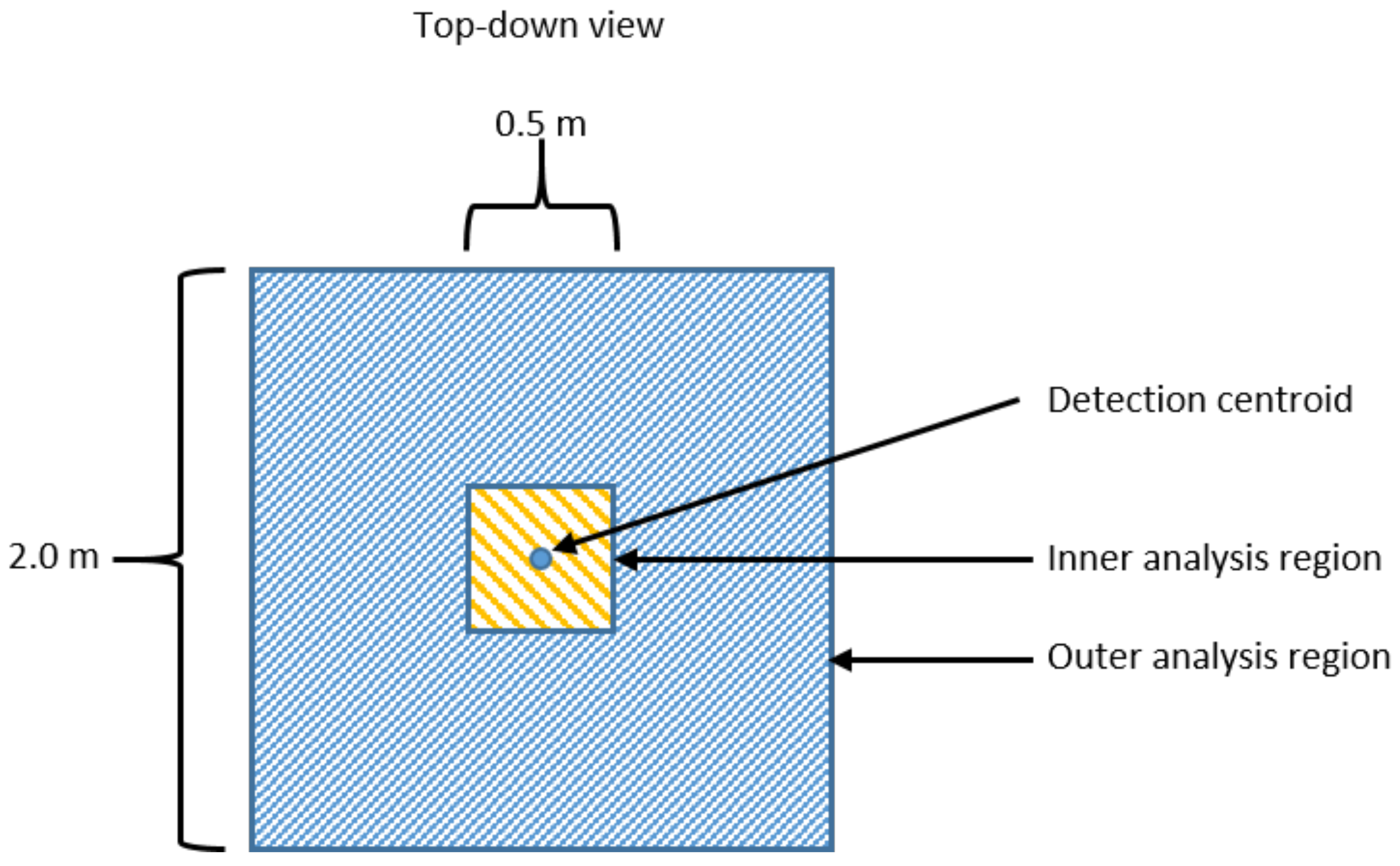
3.6.3. LiDAR Feature Extraction
| Algorithm 2: LiDAR high-level feature extraction preprocessing. |
 |
| Algorithm 3: LiDAR feature extraction. |
 |
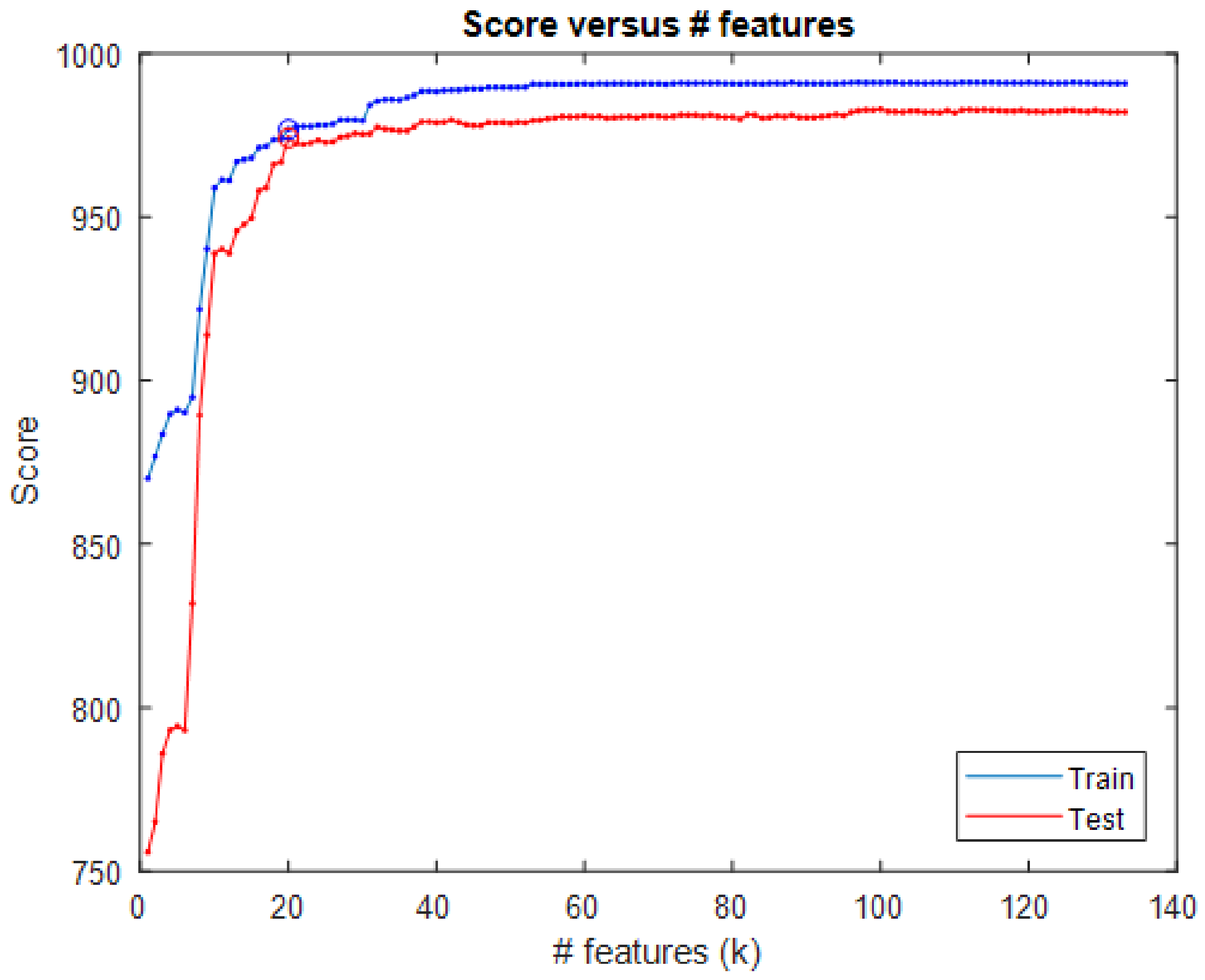
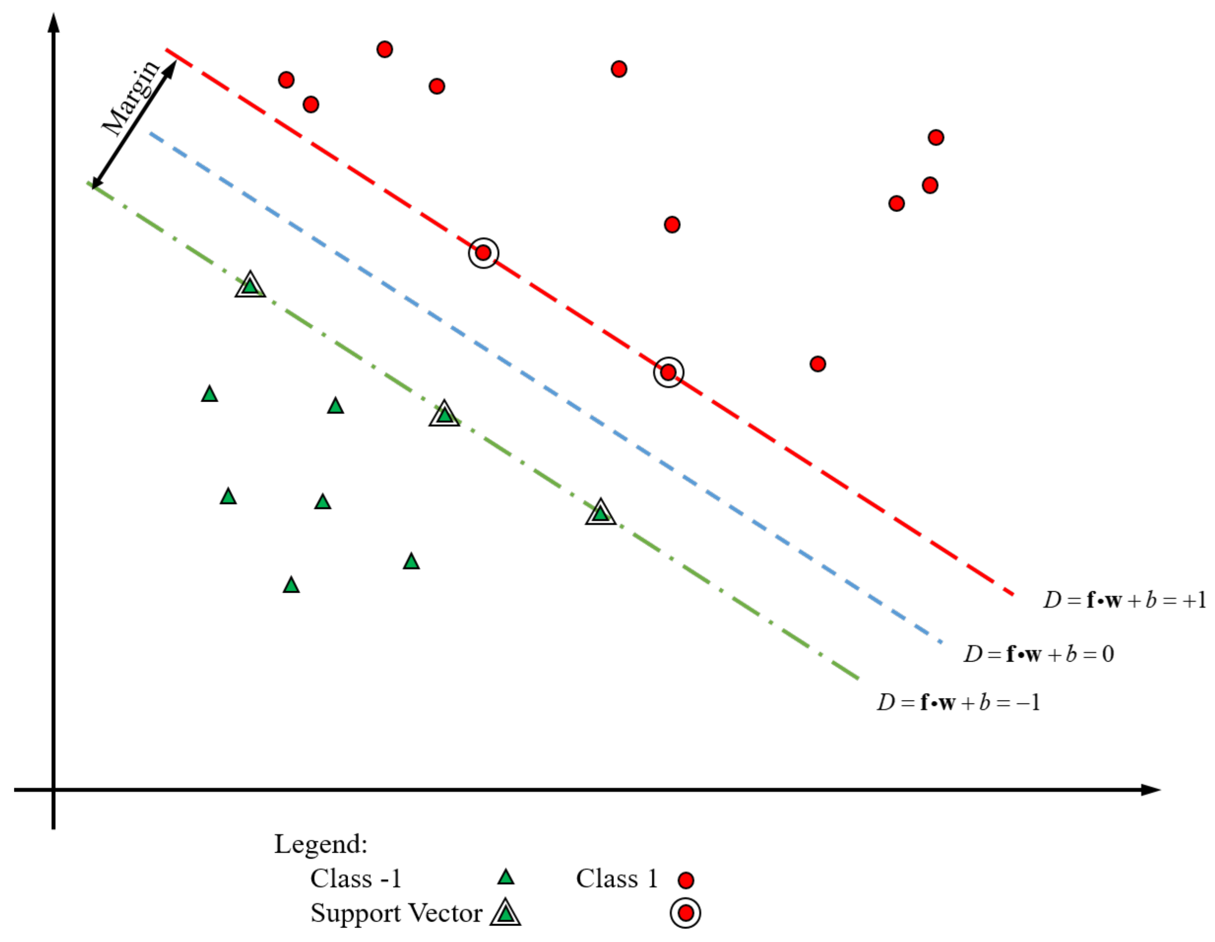
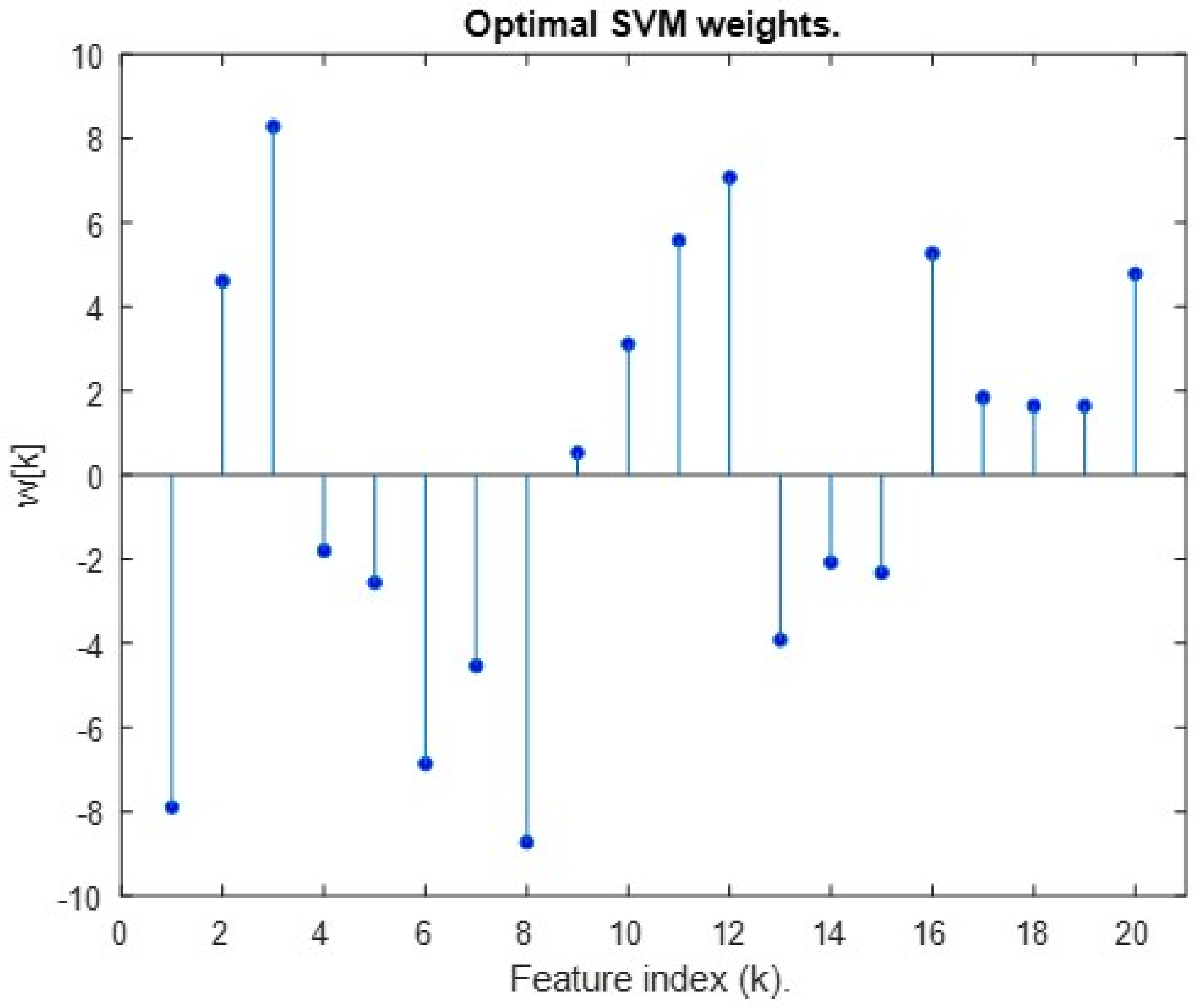
3.6.4. SVM LiDAR Beacon Detection
3.7. Mapping
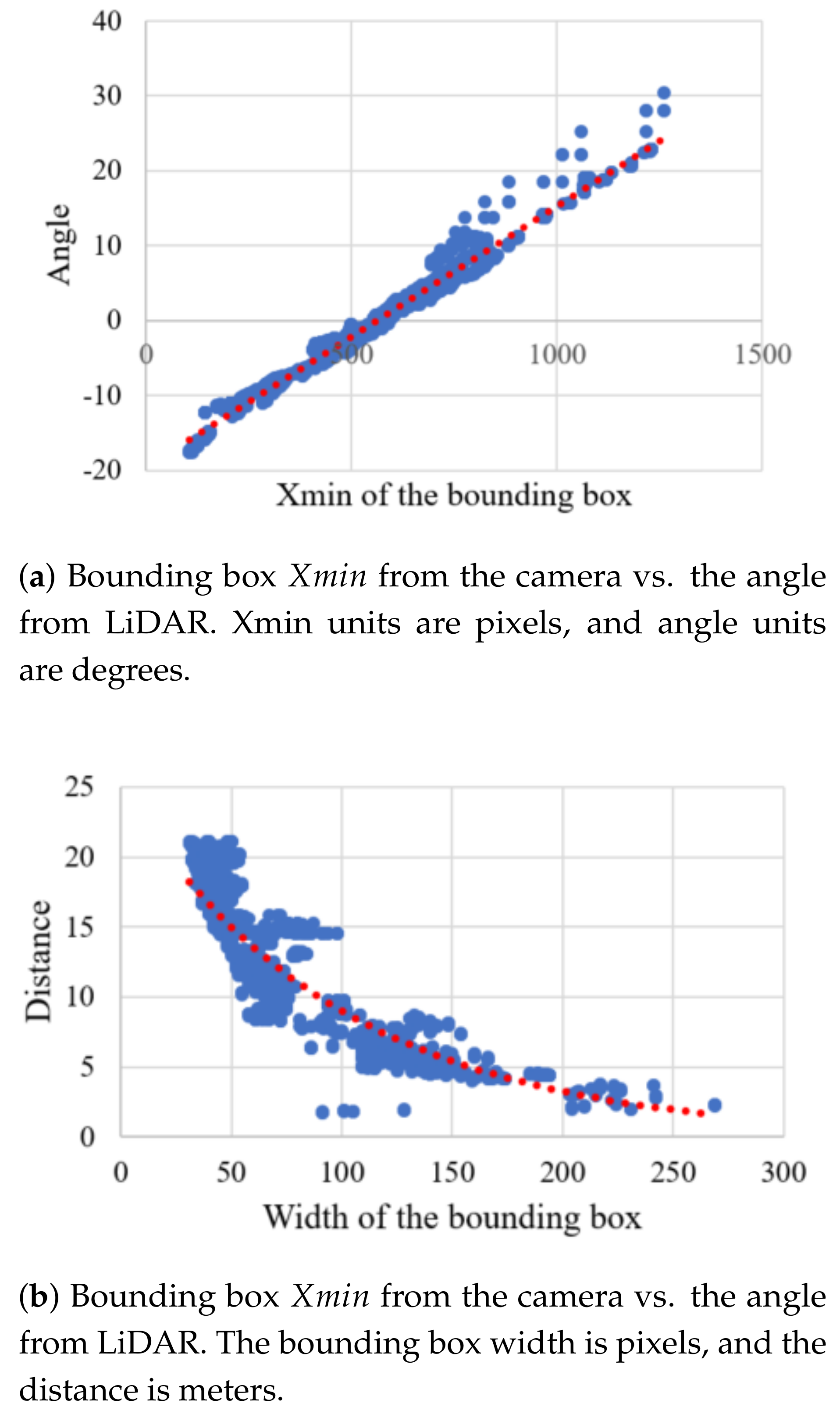
3.7.1. Camera Detection Mapping
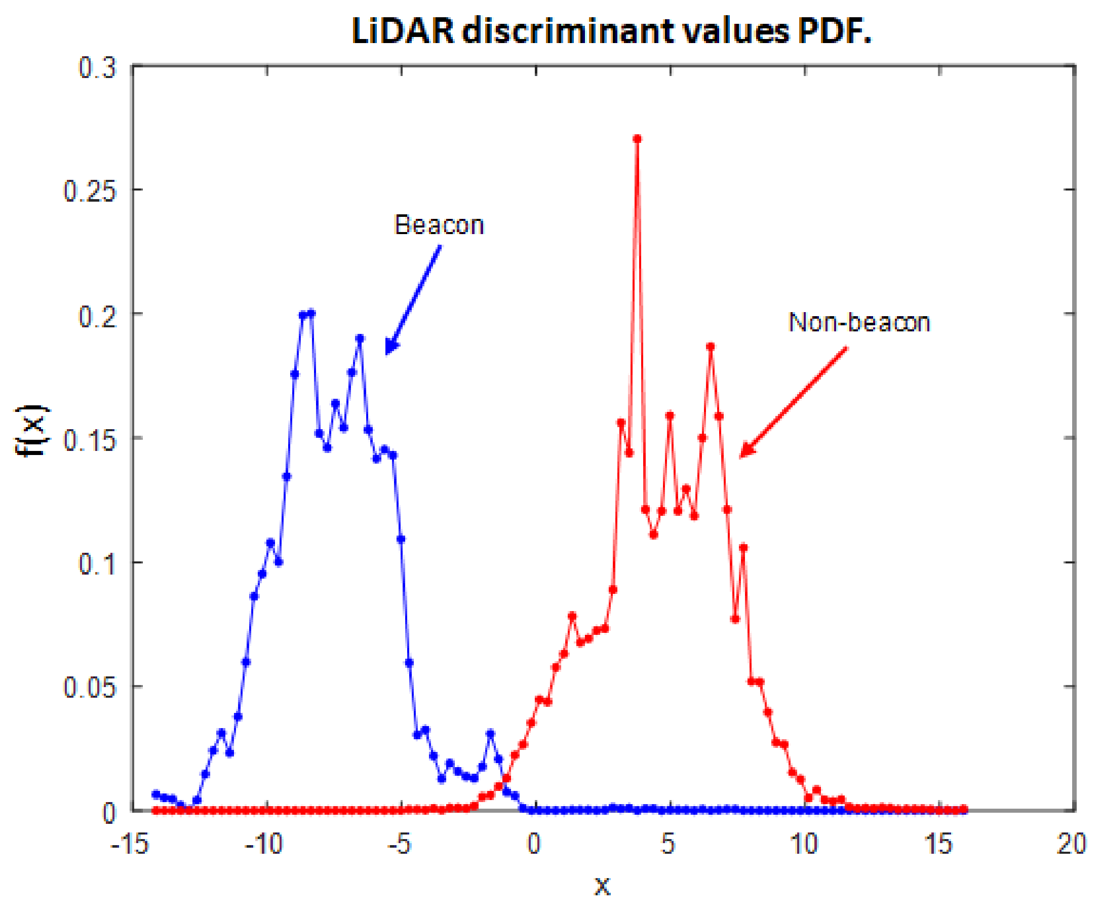
3.7.2. LiDAR Discriminate Value Mapping
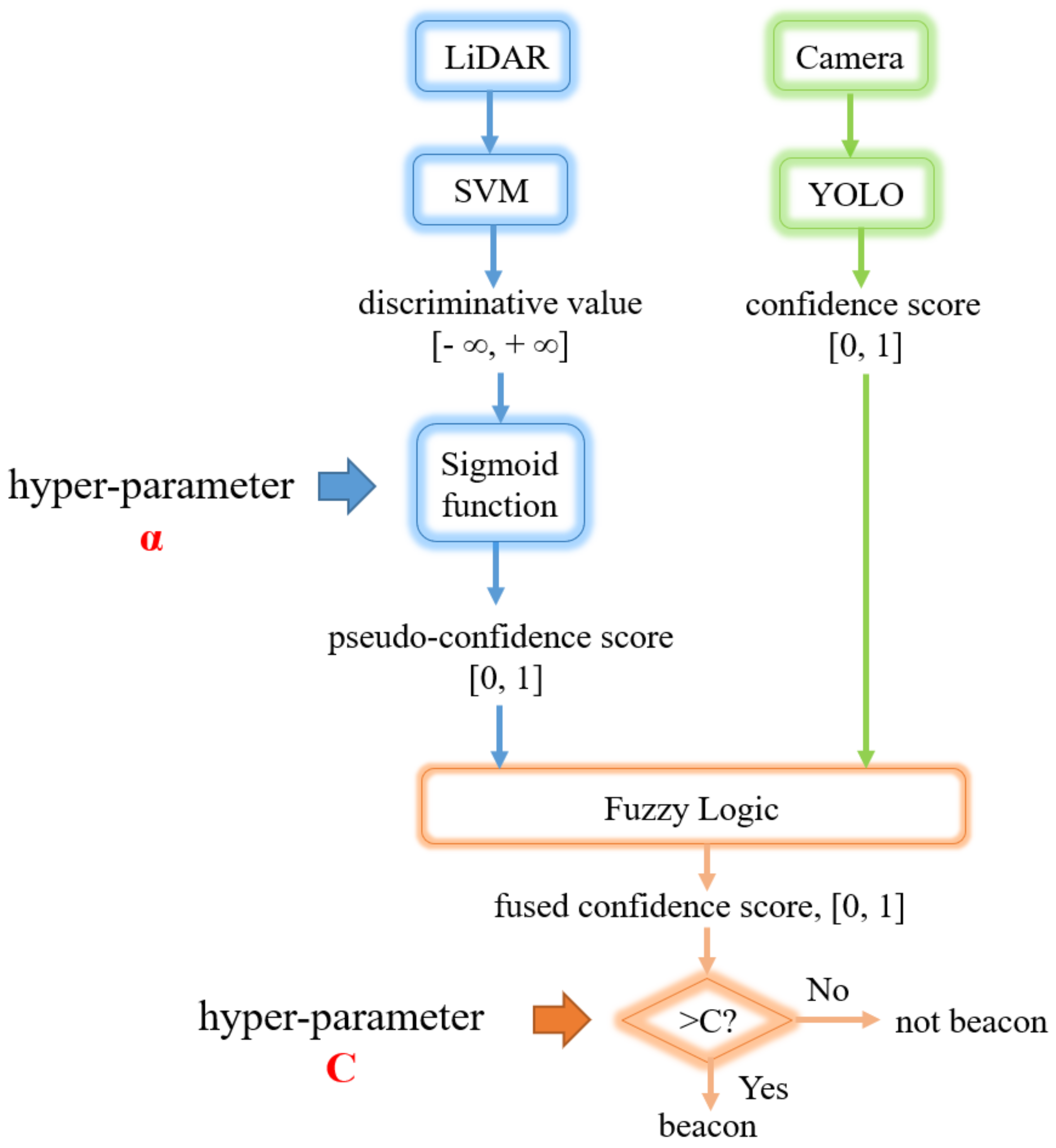
3.8. Detection Fusion
3.8.1. Fusion Algorithm
| Algorithm 4: Fusion of LiDAR and Camera detection. |
 |
- If the LiDAR confidence score is high, then the probability for detection is high.
- If the camera confidence score is high, then the probability for detection is high.
- If the LiDAR confidence score is medium, then the probability for detection is medium.
- If the LiDAR confidence score is low and the camera confidence score is medium, then the probability for detection is medium.
- If the LiDAR confidence score is low and the camera confidence score is low, then the probability for detection is low.
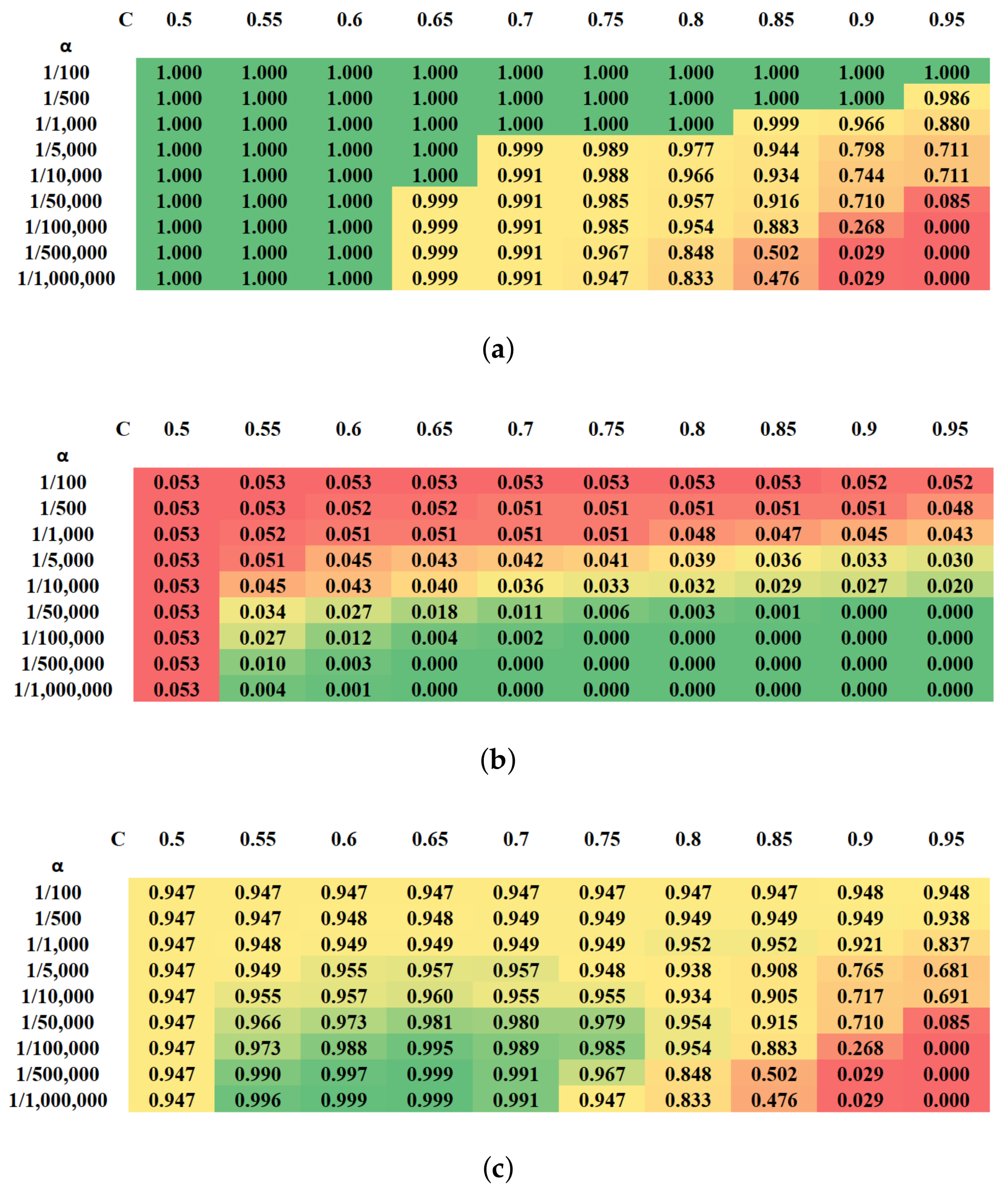
3.8.2. Hyperparameter Optimization
4. Experiment
4.1. Data Collections Summary
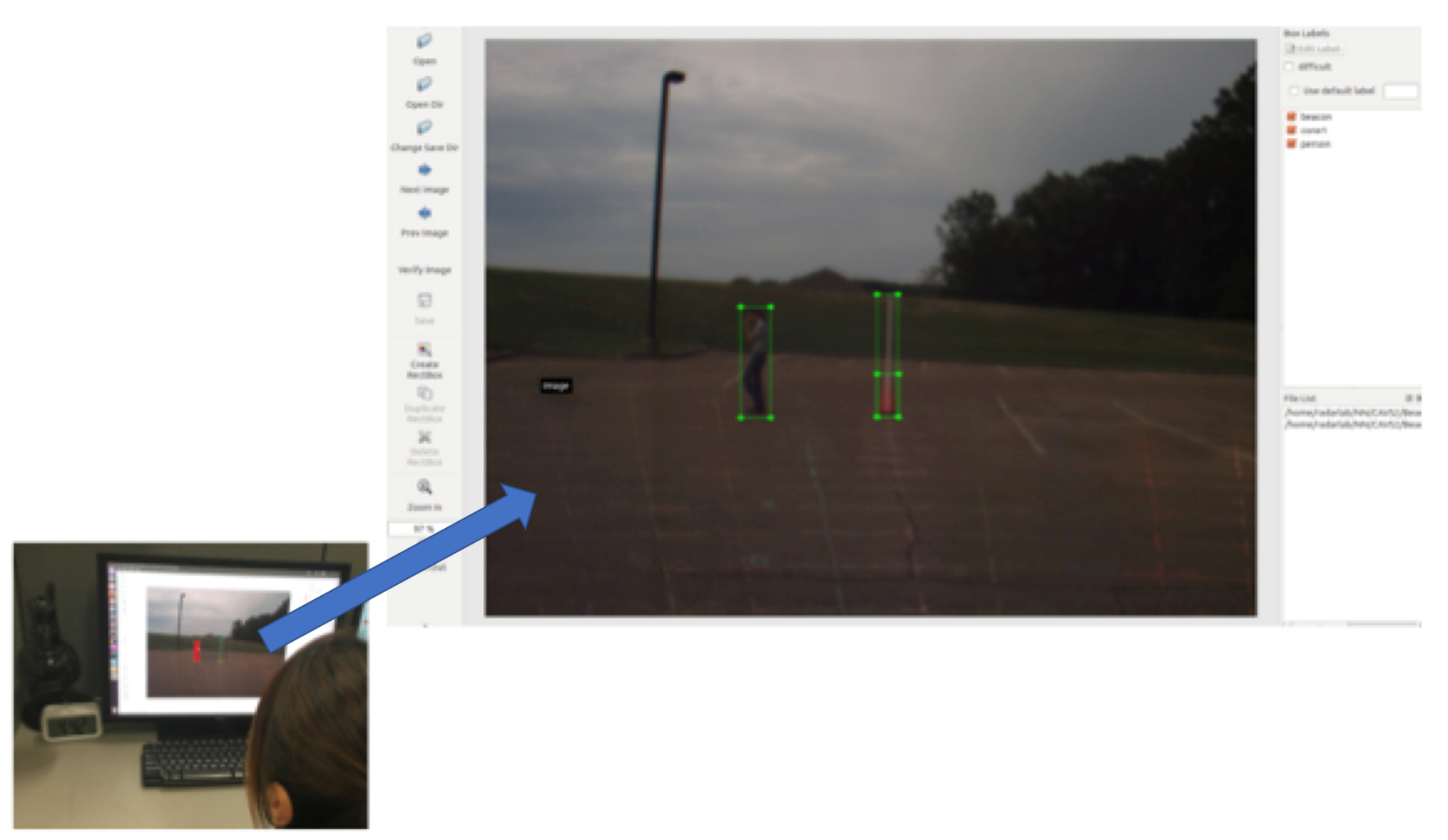
4.2. Camera Detection Training
4.3. LiDAR Detection Training
5. Results and Discussion
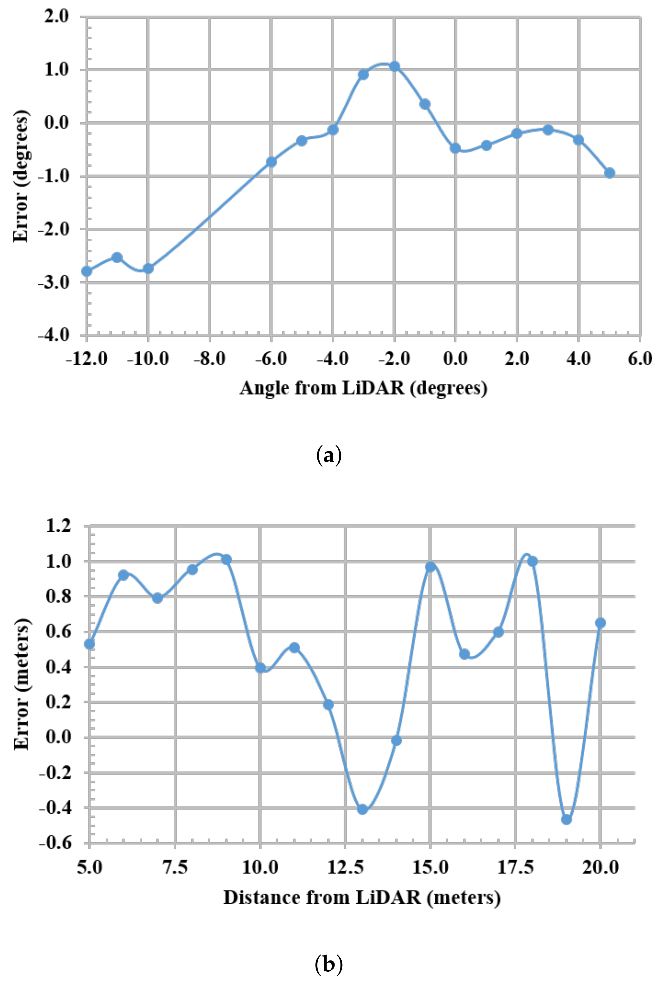
5.1. Camera Detection Mapping Results
5.2. Camera Detection Results
5.3. Fusion Results
6. Conclusions and Future Work
Author Contributions
Conflicts of Interest
References
- Redmon, J.; Divvala, S.; Girshick, R.; Farhadi, A. You Only Look Once: Unified, Real-Time Object Detection. In Proceedings of the IEEE Conference on Computer Vision and Pattern Recognition, Las Vegas, NV, USA, 27–30 June 2016; pp. 779–788. [Google Scholar]
- Redmon, J.; Farhadi, A. YOLO9000: Better, Faster, Stronger. In Proceedings of the IEEE Conference on Computer Vision and Pattern Recognition, Honolulu, HI, USA, 21–26 July 2017; pp. 6517–6525. [Google Scholar]
- Ren, S.; He, K.; Girshick, R.; Sun, J. Faster R-CNN: Towards real-time object detection with region proposal networks. IEEE Trans. Pattern Anal. Mach. Intell. 2017, 39, 1137–1149. [Google Scholar] [CrossRef] [PubMed]
- Szegedy, C.; Reed, S.; Erhan, D.; Anguelov, D.; Ioffe, S. Scalable, high-quality object detection. arXiv, 2014; arXiv:1412.1441. [Google Scholar]
- Dai, J.; Li, Y.; He, K.; Sun, J. R-FCN: Object detection via region-based fully convolutional networks. In Proceedings of the Neural Information Processing Systems 2016, Barcelona, Spain, 5–10 December 2016; pp. 379–387. [Google Scholar]
- Liu, W.; Anguelov, D.; Erhan, D.; Szegedy, C.; Reed, S.; Fu, C.Y.; Berg, A.C. SSD: Single shot multibox detector. In Proceedings of the European Conference on Computer Vision, Amsterdam, The Netherlands, 8–16 October 2016; pp. 21–37. [Google Scholar]
- Dalal, N.; Triggs, B. Histograms of Oriented Gradients for Human Detection. In Proceedings of the IEEE Computer Society Conference on Computer Vision and Pattern Recognition, San Diego, CA, USA, 20–25 June 2005; pp. 886–893. [Google Scholar]
- Felzenszwalb, P.F.; Girshick, R.B.; McAllester, D.; Ramanan, D. Object detection with discriminatively trained part-based models. IEEE Trans. Pattern Anal. Mach. Intell. 2010, 32, 1627–1645. [Google Scholar] [CrossRef] [PubMed]
- Wei, P.; Ball, J.E.; Anderson, D.T.; Harsh, A.; Archibald, C. Measuring Conflict in a Multi-Source Environment as a Normal Measure. In Proceedings of the IEEE 6th International Workshop on Computational Advances in Multi-Sensor Adaptive Processing (CAMSAP), Cancun, Mexico, 13–16 December 2015; pp. 225–228. [Google Scholar]
- Wei, P.; Ball, J.E.; Anderson, D.T. Multi-sensor conflict measurement and information fusion. In Signal Processing, Sensor/Information Fusion, and Target Recognition XXV; International Society for Optics and Photonics: Bellingham, WA, USA, 2016; Volume 9842, p. 98420F. [Google Scholar]
- Wei, P.; Ball, J.E.; Anderson, D.T. Fusion of an Ensemble of Augmented Image Detectors for Robust Object Detection. Sensors 2018, 18, 894. [Google Scholar] [CrossRef] [PubMed]
- Lin, C.H.; Chen, J.Y.; Su, P.L.; Chen, C.H. Eigen-feature analysis of weighted covariance matrices for LiDAR point cloud classification. ISPRS J. Photogr. Remote Sens. 2014, 94, 70–79. [Google Scholar] [CrossRef]
- Golovinskiy, A.; Kim, V.G.; Funkhouser, T. Shape-Based Recognition of 3D Point Clouds in Urban Environments. In Proceedings of the IEEE 12th International Conference on Computer Vision, Kyoto, Japan, 29 September–2 October 2009; pp. 2154–2161. [Google Scholar]
- Maturana, D.; Scherer, S. Voxnet: A 3d Convolutional Neural Network for Real-Time Object Recognition. In Proceedings of the IEEE/RSJ International Conference on Intelligent Robots and Systems (IROS), Hamburg, Germany, 28 September–2 October 2015; pp. 922–928. [Google Scholar]
- Wu, Z.; Song, S.; Khosla, A.; Yu, F.; Zhang, L.; Tang, X.; Xiao, J. 3d Shapenets: A Deep Representation for Volumetric Shapes. In Proceedings of the IEEE Conference on Computer Vision and Pattern Recognition, Boston, MA, USA, 7–12 June 2015; pp. 1912–1920. [Google Scholar]
- Gong, X.; Lin, Y.; Liu, J. Extrinsic calibration of a 3D LIDAR and a camera using a trihedron. Opt. Laser Eng. 2013, 51, 394–401. [Google Scholar] [CrossRef]
- Park, Y.; Yun, S.; Won, C.S.; Cho, K.; Um, K.; Sim, S. Calibration between color camera and 3D LIDAR instruments with a polygonal planar board. Sensors 2014, 14, 5333–5353. [Google Scholar] [CrossRef] [PubMed]
- García-Moreno, A.I.; Gonzalez-Barbosa, J.J.; Ornelas-Rodriguez, F.J.; Hurtado-Ramos, J.B.; Primo-Fuentes, M.N. LIDAR and panoramic camera extrinsic calibration approach using a pattern plane. In Mexican Conference on Pattern Recognition; Springer: Berlin, Germany, 2013; pp. 104–113. [Google Scholar]
- Levinson, J.; Thrun, S. Automatic Online Calibration of Cameras and Lasers. In Proceedings of the Robotics: Science and Systems, Berlin, Germany, 24–28 June 2013. [Google Scholar]
- Gong, X.; Lin, Y.; Liu, J. 3D LIDAR-camera extrinsic calibration using an arbitrary trihedron. Sensors 2013, 13, 1902–1918. [Google Scholar] [CrossRef] [PubMed]
- Napier, A.; Corke, P.; Newman, P. Cross-Calibration of Push-Broom 2d Lidars and Cameras in Natural Scenes. In Proceedings of the IEEE International Conference on Robotics and Automation (ICRA), Karlsruhe, Germany, 6–10 May 2013; pp. 3679–3684. [Google Scholar]
- Pandey, G.; McBride, J.R.; Savarese, S.; Eustice, R.M. Automatic extrinsic calibration of vision and lidar by maximizing mutual information. J. Field Robot. 2015, 32, 696–722. [Google Scholar] [CrossRef]
- Castorena, J.; Kamilov, U.S.; Boufounos, P.T. Autocalibration of LIDAR and Optical Cameras via Edge Alignment. In Proceedings of the IEEE International Conference on Acoustics, Speech and Signal Processing (ICASSP), Shanghai, China, 20–25 March 2016; pp. 2862–2866. [Google Scholar]
- Li, J.; He, X.; Li, J. 2D LiDAR and Camera Fusion in 3D Modeling of Indoor Environment. In Proceedings of the IEEE National Aerospace and Electronics Conference (NAECON), Dayton, OH, USA, 15–19 June 2015; pp. 379–383. [Google Scholar]
- Zhang, Q.; Pless, R. Extrinsic Calibration of a Camera and Laser Range Finder (Improves Camera Calibration). In Proceedings of the IEEE/RSJ International Conference on Intelligent Robots and Systems, Sendai, Japan, 28 September–2 October 2004; pp. 2301–2306. [Google Scholar]
- Vasconcelos, F.; Barreto, J.P.; Nunes, U. A minimal solution for the extrinsic calibration of a camera and a laser-rangefinder. IEEE Trans. Pattern Anal. Mach. Intell. 2012, 34, 2097–2107. [Google Scholar] [CrossRef] [PubMed]
- Mastin, A.; Kepner, J.; Fisher, J. Automatic Registration of LIDAR and Optical Images of Urban Scenes. In Proceedings of the IEEE Conference on Computer Vision and Pattern Recognition, Miami, FL, USA, 20–25 June 2009; pp. 2639–2646. [Google Scholar]
- Maddern, W.; Newman, P. Real-Time Probabilistic Fusion of Sparse 3D LIDAR and Dense Stereo. In Proceedings of the IEEE/RSJ International Conference on Intelligent Robots and Systems (IROS), Daejeon, Korea, 9–14 October 2016; pp. 2181–2188. [Google Scholar]
- Zadeh, L.A. Fuzzy sets. Inf. Control 1965, 8, 338–353. [Google Scholar] [CrossRef]
- Ross, T.J. Fuzzy Logic with Engineering Applications; John Wiley & Sons: Hoboken, NJ, USA, 2010. [Google Scholar]
- Zhao, G.; Xiao, X.; Yuan, J. Fusion of Velodyne and Camera Data for Scene Parsing. In Proceedings of the 15th International Conference on Information Fusion (FUSION), Singapore, 9–12 July 2012; pp. 1172–1179. [Google Scholar]
- Liu, J.; Jayakumar, P.; Stein, J.; Ersal, T. A Multi-Stage Optimization Formulation for MPC-based Obstacle Avoidance in Autonomous Vehicles Using a LiDAR Sensor. In Proceedings of the ASME Dynamic Systems and Control Conference, Columbus, OH, USA, 28–30 October 2015. [Google Scholar]
- Alrifaee, B.; Maczijewski, J.; Abel, D. Sequential Convex Programming MPC for Dynamic Vehicle Collision Avoidance. In Proceedings of the IEEE Conference on Control TEchnology and Applications, Mauna Lani, HI, USA, 27–30 August 2017. [Google Scholar]
- Anderson, S.J.; Peters, S.C.; Pilutti, T.E.; Iagnemma, K. An Optimal-control-based Framework for Trajectory Planning, Thread Assessment, and Semi-Autonomous Control of Passenger Vehicles in Hazard Avoidance Scenarios. Int. J. Veh. Auton. Syst. 2010, 8, 190–216. [Google Scholar] [CrossRef]
- Liu, Y.; Davenport, C.; Gafford, J.; Mazzola, M.; Ball, J.; Abdelwahed, S.; Doude, M.; Burch, R. Development of A Dynamic Modeling Framework to Predict Instantaneous Status of Towing Vehicle Systems; SAE Technical Paper; SAE International: Warrendale, PA, USA; Troy, MI, USA, 2017. [Google Scholar]
- Davenport, C.; Liu, Y.; Pan, H.; Gafford, J.; Abdelwahed, S.; Mazzola, M.; Ball, J.E.; Burch, R.F. A kinematic modeling framework for prediction of instantaneous status of towing vehicle systems. SAE Int. J. Passeng. Cars Mech. Syst. 2018. [Google Scholar] [CrossRef]
- Quigley, M.; Gerkey, B.; Conley, K.; Faust, J.; Foote, T.; Leibs, J.; Berger, E.; Wheeler, R.; Ng, A. ROS: An open-source Robot Operating System. In Proceedings of the IEEE Conference on Robotics and Automation (ICRA) Workshop on Open Source Robotics, Kobe, Japan, 12–17 May 2009. [Google Scholar]
- ROS Nodelet. Available online: http://wiki.ros.org/nodelet (accessed on 22 April 2018).
- JETSON TX2 Technical Specifications. Available online: https://www.nvidia.com/en-us/autonomousmachines/embedded-systems-dev-kits-modules/ (accessed on 5 March 2018).
- Girshick, R. Fast R-CNN. arXiv, 2015; arXiv:1504.08083. [Google Scholar]
- Ester, M.; Kriegel, H.P.; Sander, J.; Xu, X. A density-based algorithm for discovering clusters in large spatial databases with noise. In Proceedings of the Second International Conference on Knowledge Discovery and Data Mining, Portland, OR, USA, 2–4 August 1996; pp. 226–231. [Google Scholar]
- Wang, L.; Zhang, Y. LiDAR Ground Filtering Algorithm for Urban Areas Using Scan Line Based Segmentation. arXiv, 2016; arXiv:1603.00912. [Google Scholar]
- Meng, X.; Currit, N.; Zhao, K. Ground filtering algorithms for airborne LiDAR data: A review of critical issues. Remote Sens. 2010, 2, 833–860. [Google Scholar] [CrossRef]
- Rummelhard, L.; Paigwar, A.; Nègre, A.; Laugier, C. Ground estimation and point cloud segmentation using SpatioTemporal Conditional Random Field. In Proceedings of the Intelligent Vehicles Symposium (IV), Los Angeles, CA, USA, 11–14 June 2017; pp. 1105–1110. [Google Scholar]
- Rashidi, P.; Rastiveis, H. Ground Filtering LiDAR Data Based on Multi-Scale Analysis of Height Difference Threshold. Int. Arch. Photogramm. Remote Sens. Spat. Inf. Sci. 2017, XLII-4/W4, 225–229. [Google Scholar] [CrossRef]
- Chang, Y.; Habib, A.; Lee, D.; Yom, J. Automatic classification of lidar data into ground and non-ground points. Int. Arch. Photogr. Remote Sens. 2008, 37, 463–468. [Google Scholar]
- Miadlicki, K.; Pajor, M.; Saków, M. Ground plane estimation from sparse LIDAR data for loader crane sensor fusion system. In Proceedings of the 2017 22nd International Conference on Methods and Models in Automation and Robotics (MMAR), Miedzyzdroje, Poland, 28–31 August 2017; pp. 717–722. [Google Scholar]
- Lillywhite, K.; Lee, D.J.; Tippetts, B.; Archibald, J. A feature construction method for general object recognition. Pattern Recognit. 2013, 46, 3300–3314. [Google Scholar] [CrossRef]
- Vapnik, V. Statistical Learning Theory; Wiley: New York, NY, USA, 1998. [Google Scholar]
- Fan, R.; Chang, K.; Hsieh, C. LIBLINEAR: A library for large linear classification. J. Mach. Learn. Res. 2008, 9, 1871–1874. [Google Scholar]
- Zorzi, M.; Chiuso, A. Sparse plus low rank network identification: A nonparametric approach. Automatica 2017, 76, 355–366. [Google Scholar] [CrossRef]
- Chicco, D. Ten quick tips for machine learning in computational biology. BioData Min. 2017, 10, 35. [Google Scholar] [CrossRef] [PubMed]
- Hsu, C.W.; Chang, C.C.; Lin, C.J. A Practical Guide to Support Vector Classification; Technical Report; National Taiwan University: Taiwan, China, 2010. [Google Scholar]
- Olson, R.S.; Urbanowicz, R.J.; Andrews, P.C.; Lavender, N.A.; Moore, J.H. Automating biomedical data science through tree-based pipeline optimization. In Proceedings of the European Conference on the Applications of Evolutionary Computation, Porto, Portugal, 30 March–1 April 2016; pp. 123–137. [Google Scholar]
- Chakravarty, I.M.; Roy, J.; Laha, R.G. Handbook of Methods of Applied Statistics; McGraw-Hill: New York, NY, USA, 1967. [Google Scholar]
- Everingham, M.; Van Gool, L.; Williams, C.K.; Winn, J.; Zisserman, A. The pascal visual object classes (voc) challenge. Int. J. Comput. Vis. 2010, 88, 303–338. [Google Scholar] [CrossRef]
- Draper, N.R.; Smith, H. Applied Regression Analysis; John Wiley & Sons: Hoboken, NJ, USA, 2014; Volume 326. [Google Scholar]
- Larochelle, V.; Bonnier, D.; Roy, G.; Simard, J.R.; Mathieu, P. Performance assessment of various imaging sensors in fog. In Proceedings of the International Society for Optical Engineering, Aspen, CO, USA, 10–13 May 1998; pp. 66–81. [Google Scholar]
- Park, D.; Ko, H. Fog-degraded image restoration using characteristics of RGB channel in single monocular image. In Proceedings of the IEEE International Conference on Consumer Electronics, Las Vegas, NV, USA, 13–16 January 2012; pp. 139–140. [Google Scholar]


| Feature Number | Data Subset | Analysis Region | Description |
|---|---|---|---|
| 1 | HT | Inner | Extent of Z in cluster. Extent {Z} = max{Z} − min{Z}. |
| 2 | LT | Outer | Max of X and Y extents in cluster, Beam 7. This is max{extent{X}, extent{Y}}. Extent {X} = max{X} − min{X}. Extent {Y} = max{Y} − min{Y}. |
| 3 | LT | Outer | Max of X and Y extents in cluster, Beam 5. This is max{extent{X}, extent{Y}}. Extent {X} = max{X} − min{X}. Extent {Y} = max{Y} − min{Y}. |
| 4 | HT | Outer | Max{Z in cluster - LiDAR height}. Z is vertical (height) of LiDAR return. |
| 5 | LT | Outer | Extent of Z in cluster. Extent{Z}= max{Z} − min{Z}. |
| 6 | LT | Inner | Number of valid points in cluster, Beam 7. |
| 7 | LT | Inner | Max of X and Y extents in cluster, Beam 6. This is max{extent{X}, extent{Y}}. Extent {X} = max{X} − min{X}. Extent {Y} = max{Y} − min{Y}. |
| 8 | LT | Outer | Number of points in cluster, Beam 5. |
| 9 | LT | Inner | Extent of X in cluster. Extent{X} = max{X} − min{X}. |
| 10 | LT | Inner | Number of points in cluster, Beam 4. |
| 11 | LT | Inner | Number of points in cluster, Beam 5. |
| 12 | LT | Outer | Number of points in cluster, Beam 6. |
| 13 | HT | Inner | Number of points in cluster, Beam 6. |
| 14 | LT | Inner | Max of X and Y extents, Beam 5. This is max{extent{X}, extent{Y}}. Extent {X} = max{X} − min{X}. Extent {Y} = max{Y} − min{Y}. |
| 15 | LT | Outer | Number of points in cluster divided by the cluster radius in Beam 5. |
| 16 | LT | Inner | Extent of X in cluster. Extent {X} = max{X} − min{X}. |
| 17 | HT | Inner | Number of points in cluster, Beam 7. |
| 18 | LT | Inner | Number of points in cluster. |
| 19 | LT | Outer | Number of points in cluster. |
| 20 | LT | Outer | Extent of Z in cluster. Extent {Y} = max{Y} − min{Y}. |
| Beacon | Non-Beacon | |
|---|---|---|
| Beacon | 13,158 | 32 |
| Non-Beacon | 610 | 14,599 |
| Beacon | Non-Beacon | |
|---|---|---|
| Beacon | 5653 | 13 |
| Non-Beacon | 302 | 11,782 |
| Angle (Degrees) | Distance (Meters) | |||
|---|---|---|---|---|
| NN | Linear Regression | NN | Exponential Curve Fitting | |
| Mean Squared Error (MSE) | 0.0467 | 0.0468 | 0.0251 | 0.6278 |
| r2 score | 0.9989 | 0.9989 | 0.9875 | 0.9687 |
| LiDAR Only | Camera Only | Fusion | |
|---|---|---|---|
| True Positive Rate (TPR) | 93.90% | 97.60% | 97.60% |
| False Positive Rate (FPR) | 27.00% | 0.00% | 6.69% |
| False Negative Rate (FNR) | 6.10% | 2.40% | 2.40% |
| Camera Only | Fusion | |
|---|---|---|
| True Positive Rate (TPR) | 94.80% | 94.80% |
| False Positive Rate (FPR) | 0.00% | 0.00% |
| False Negative Rate (FNR) | 5.20% | 5.20% |
© 2018 by the authors. Licensee MDPI, Basel, Switzerland. This article is an open access article distributed under the terms and conditions of the Creative Commons Attribution (CC BY) license (http://creativecommons.org/licenses/by/4.0/).
Share and Cite
Wei, P.; Cagle, L.; Reza, T.; Ball, J.; Gafford, J. LiDAR and Camera Detection Fusion in a Real-Time Industrial Multi-Sensor Collision Avoidance System. Electronics 2018, 7, 84. https://doi.org/10.3390/electronics7060084
Wei P, Cagle L, Reza T, Ball J, Gafford J. LiDAR and Camera Detection Fusion in a Real-Time Industrial Multi-Sensor Collision Avoidance System. Electronics. 2018; 7(6):84. https://doi.org/10.3390/electronics7060084
Chicago/Turabian StyleWei, Pan, Lucas Cagle, Tasmia Reza, John Ball, and James Gafford. 2018. "LiDAR and Camera Detection Fusion in a Real-Time Industrial Multi-Sensor Collision Avoidance System" Electronics 7, no. 6: 84. https://doi.org/10.3390/electronics7060084
APA StyleWei, P., Cagle, L., Reza, T., Ball, J., & Gafford, J. (2018). LiDAR and Camera Detection Fusion in a Real-Time Industrial Multi-Sensor Collision Avoidance System. Electronics, 7(6), 84. https://doi.org/10.3390/electronics7060084