Review of Polynomial Chaos-Based Methods for Uncertainty Quantification in Modern Integrated Circuits


Abstract
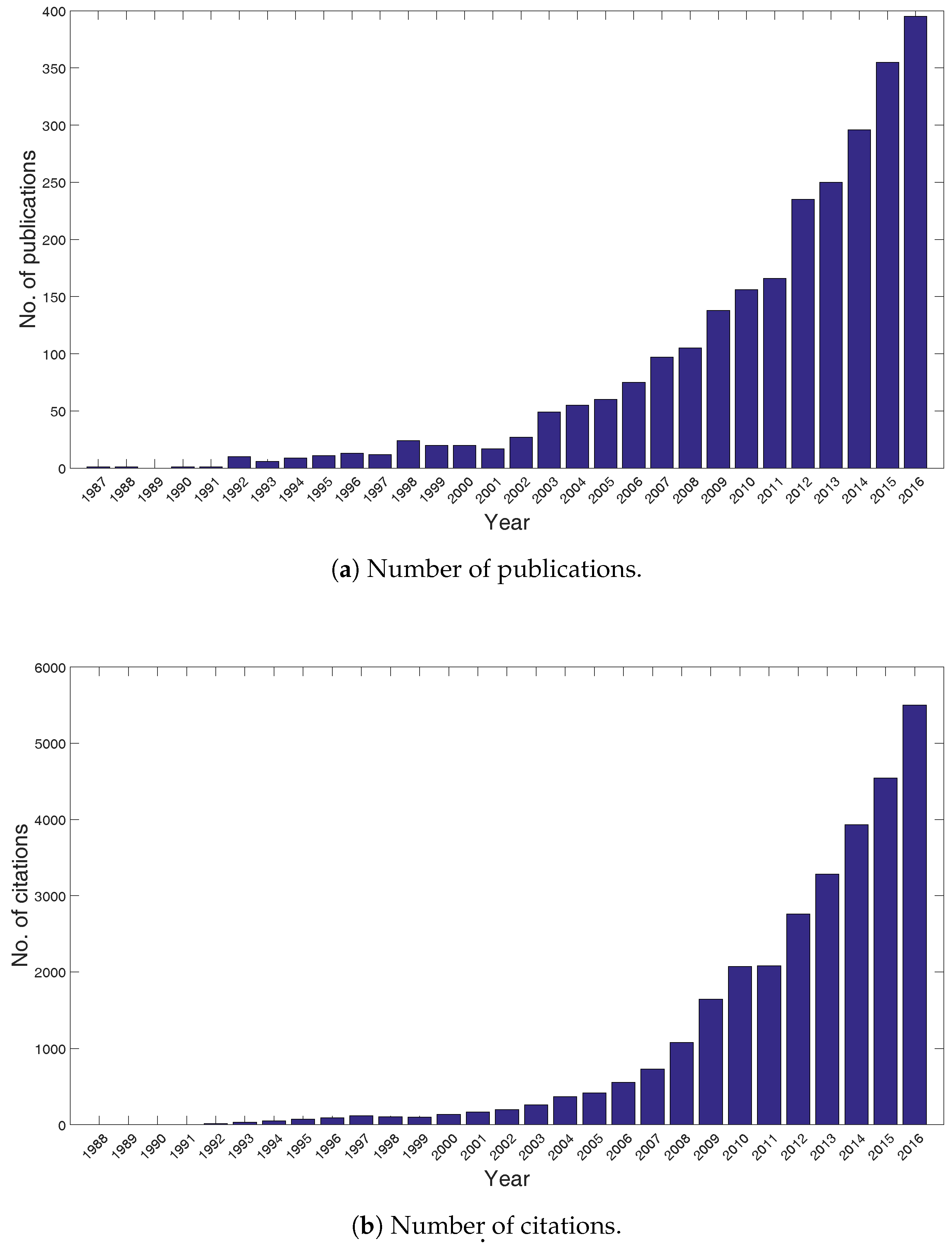
:1. Introduction
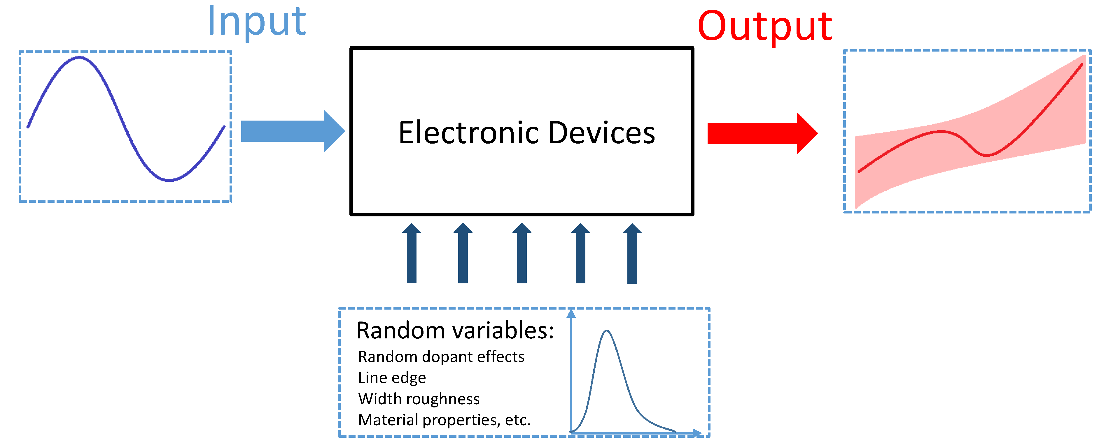
2. Problem Setting
3. Polynomial Chaos Expansion
3.1. Preliminaries: PC Properties
3.2. Computing a PC Model
4. PC-Based Applications in Electronics
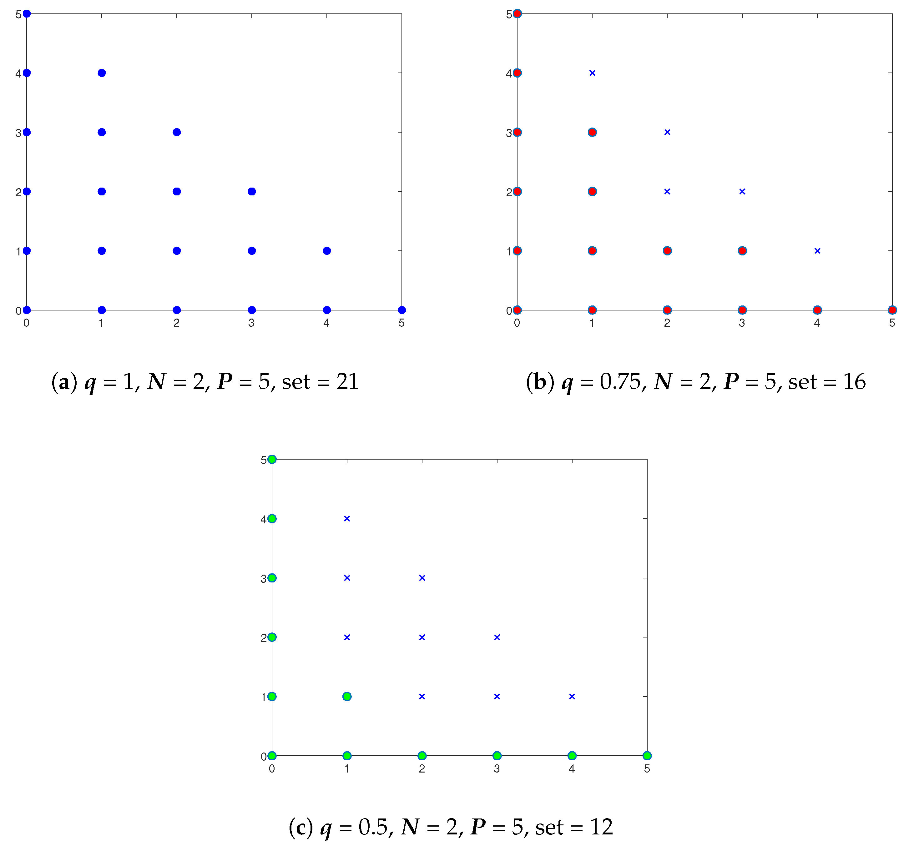
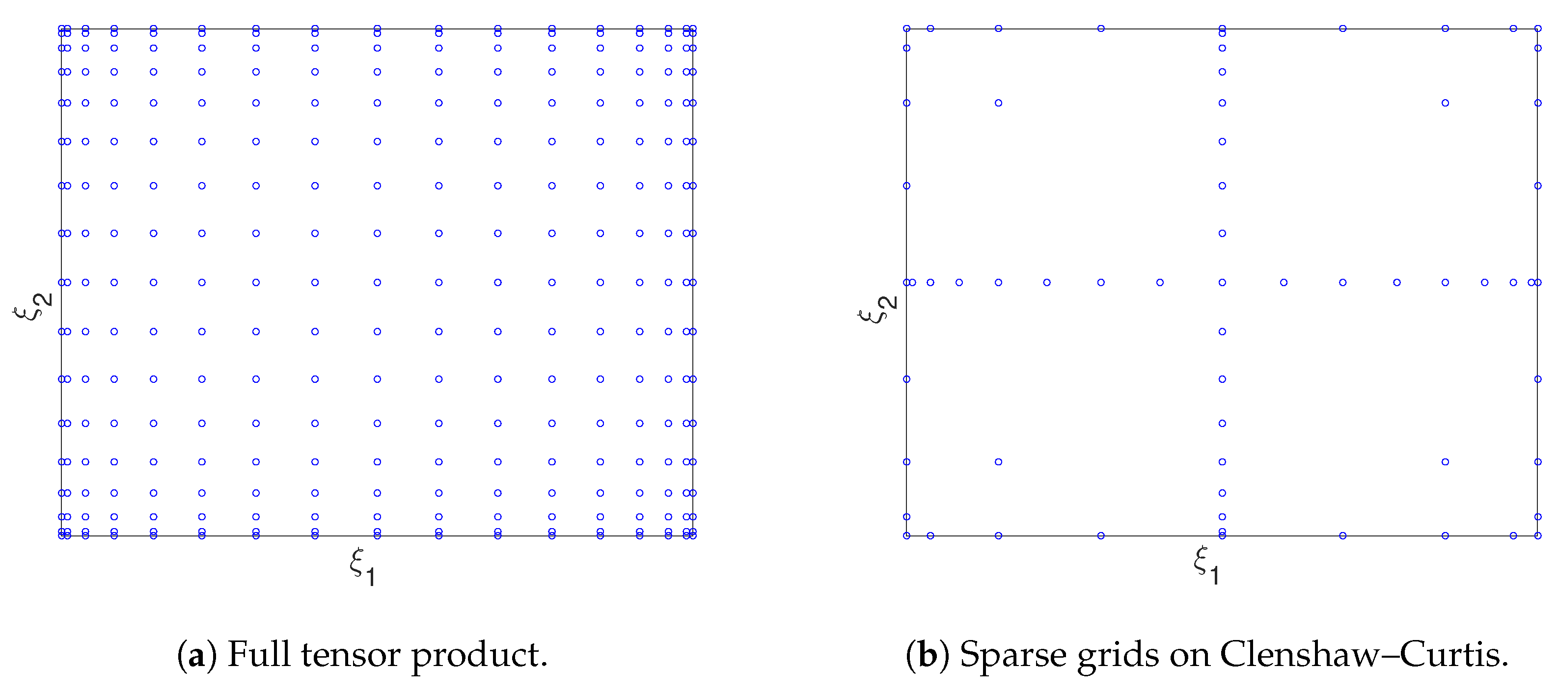
- Spectral Projection or Collocation Approach: By definition, the PC coefficients can be expressed as [13,23]Note that Equation (17) can be directly obtained by projecting Equation (3) onto each basis function for and by employing the orthonormal relation of Equation (4) (where in Equation (4) for orthonormal basis functions). Now, the inner product in Equation (17) can be written as a suitable multi-dimensional integral (see Equation (4)):In general, it is not possible to solve Equation (18) analytically, but numerical integration techniques can be adopted. Indeed, let us consider a set of values of the random variables , indicated with for , and the corresponding deterministic solutions ; Equation (18) can then be expressed aswhere the values for (also called quadrature points) and corresponding weights depend on the particular numerical method adopted [60]. For example, the tensor-product approach is an efficient technique when the number of random variables is small, whereas sparse grid techniques (e.g., the Smolyak algorithm [61]) are proved to be more efficient for a large number of random variables (see Appendix A). Note that various adaptive methods for quadrature node selection have also been introduced in the literature: for example, in [62], an adaptive algorithm based on nested sparse grids is proposed and applied to a stochastic eddy current NDT problems, a weighted Smolyak algorithm is presented in [63], an adaptive hierarchical sparse grid collocation algorithm and a data-driven sparse grid approach are illustrated in [64,65], respectively. In conclusion, a spectral projection can be considered as a nonintrusive strategy, requiring a suitable deterministic problem to be solved times [23,66].
- Linear regression is a nonintrusive approach whereby the PC coefficients are computed via a suitable least square problem [23,54,55]. Indeed, let us consider again a set of samples of our random variables for , the corresponding values of the basis functions and of the stochastic process . Now, by looking at Equation (3), a suitable linear system can be written aswhere and contain the basis functions and realizations computed for the chosen values of the random variables, respectively, and collects the PC coefficients to be determined.If the number of samples is greater than the unknown PC coefficients, then the system (20) is over-determined and can be solved as a least square problem [54]. Generally, a value is considered to be sufficient for a robust solution and to prevent overfitting [67]. Linear regression has been a popular technique to determine the PC coefficients in various stochastic problems in circuit analysis. However, the choice of the regression nodes highly impact the accuracy of the results. As a result, various criteria have been proposed in the literature, such as random sampling and Latin Hypercube-based approaches [68], which suffer from slow convergence. An efficient D-optimal approach based on the optimization of a suitable information matrix has been proposed [69]. Moreover, a sparse linear regression method for high-speed circuits based on the modified Fedorov search algorithm is described in [70], which utilizes comparatively few regression nodes for the PC coefficient computation. Linear regression has been used with optimal regression nodes based on D-optimal design for microwave/RF networks in a multi-dimensional UQ framework [71]. In [72], the regression nodes are selected by a non-adaptive quasi-optimal technique (for least squares linear regression), which maximizes a parameter based on the mutual column orthogonality and the determinant of the model matrix. Various coherence-based random sampling schemes has also been derived from the properties of Hermite and Legendre polynomials as proposed in [73].
- The Galerkin Projection method is an intrusive method for evaluating the desired PC coefficients. As already mentioned, it generates a coupled system of deterministic equations where the PC coefficients are the unknowns, and these equations can be solved by using suitable numerical methods. Indeed, let us consider a general system of equations in the form of Equation (1). Expressing the quantities in Equation (1) depending on the random variables by means of the PC expansion leads toNow, it is possible to project Equation (21) onto each PC basis function asNote that starting from the initial stochastic problem of Equation (1), we have obtained a system of coupled deterministic equations in the form of Equation (22). Indeed, the projection operator <> requires integration of the quantity of interest with respect to the random variables in the stochastic space , as shown in Equations (4) and (18). By solving such system of equations, the desired PC coefficients can be determined. In particular, the obtained coupled system of equations has the same form of the original problem of Equation (1) when no stochastic effects are present: this problem can be solved by means of the same methods applicable to the “original” problem under study, depending on the type of (linear or nonlinear) operator considered. Using the Galerkin Projection method offers an elegant way of computing the PC coefficients, allowing its application to a wide variety of problems. For example, such an intrusive approach has been adopted to solve transmission lines [47,74] or stochastic full wave [75] problems. However, using the Galerkin method poses some challenges: Formulating and solving the obtained coupled system of equations for the determination of PC coefficients could be a difficult task. Furthermore, the method, for problems with a high-dimensional random space [76,77] or when complex mathematical equations are considered, can result in a significant computational cost.
- Stochastic Testing in [38,58], an efficient and accurate algorithm, was introduced for the UQ of transistor-level circuits, which has been implemented in a SPICE-type stochastic simulator. It utilizes a suitable set of values of the random variables to generate a new system of deterministic coupled equations as a function of the PC coefficients, starting from the initial stochastic equations. The first step is to select testing nodes for (also known as collocation points) from a large pool of candidate nodes generated by a suitable collocation scheme (such as tensor product or sparse grid method [60], see the discussion in the collocation approach above). The most important nodes are then selected based on the testing node scheme in [38]. Hence, Equation (21) can be formulated aswhere is the residual function and is the vector of the PC coefficients such that for . Finally, a system of coupled algebraic equations is generated by enforcing the residual function to be zero at each of the testing nodes. The resulting equation can then be directly solved by the stochastic testing solver in an intrusive way in order to estimate the PC coefficients.One of the advantages of stochastic testing method over other approaches is its efficiency. Indeed, this method employs an efficient testing node scheme that significantly reduces the required number of samples in comparison to the traditional tensor-product and sparse grid-based methods [22,60]): . Moreover, a decoupling procedure applied inside the intrusive solver makes the stochastic testing method computationally more efficient than Galerkin-based approaches [38,58]. A nonintrusive formulation of the stochastic testing approach has been presented in [59], while in [78], the stochastic testing method is applied to evaluate the performance of a wireless links under the influence of a large number of random variables in a nonintrusive manner.
5. High-Dimensional Problems
5.1. Efficient Sampling Strategies for High-Dimensional Problems
5.2. Optimization of PC Models
6. Conclusions
Author Contributions
Conflicts of Interest
Appendix A. Numerical Quadrature

References
- Moore, G.E. Cramming more components onto integrated circuits. Electronics 1965, 38, 114–117. [Google Scholar] [CrossRef]
- Dhia, S.B.; Ramdani, M.; Sicard, E. Electromagnetic Compatibility of Integrated Circuits: Techniques for Low Emission and Susceptibility; Springer: New York, NJ, USA, 2005. [Google Scholar]
- Maly, W. Cost of Silicon Viewed from VLSI Design Perspective. In Proceedings of the 31st Design Automation Conference, San Diego, CA, USA, 6–10 June 1994. [Google Scholar]
- Iwai, H.; Kakushima, K.; Wong, H. Challenges for Future Semiconductor Manufacturing. Int. J. High Speed Electron. Syst. 2006, 16, 43–81. [Google Scholar] [CrossRef]
- Nassif, S.R. Modeling and analysis of manufacturing variations. In Proceedings of the IEEE 2001 Custom Integrated Circuits Conference, San Diego, CA, USA, 9 May 2001; pp. 223–228. [Google Scholar]
- Boning, D.S.; Balakrishnan, K.; Cai, H.; Drego, N.; Farahanchi, A.; Gettings, K.M.; Lim, D.; Somani, A.; Taylor, H.; Truque, D.; et al. Variation. IEEE Trans. Semicond. Manuf. 2008, 21, 63–71. [Google Scholar] [CrossRef]
- Tega, N.; Miki, H.; Pagette, F.; Frank, D.J.; Ray, A.; Rooks, M.J.; Haensch, W.; Torii, K. Increasing threshold voltage variation due to random telegraph noise in FETs as gate lengths scale to 20 nm. In Proceedings of the Symposium on VLSI Technology, Honolulu, HI, USA, 16–18 June 2009; pp. 50–51. [Google Scholar]
- Gong, F.; Liu, X.; Yu, H.; Tan, S.X.D.; Ren, J.; He, L. A Fast Non-Monte-Carlo Yield Analysis and Optimization by Stochastic Orthogonal Polynomials. ACM Trans. Des. Autom. Electron. Syst. 2012, 17, 10. [Google Scholar] [CrossRef]
- Bai, E.W. Adaptive quantification of model uncertainties by rational approximation. IEEE Trans. Autom. Control 1991, 36, 441–453. [Google Scholar] [CrossRef]
- De Vries, D.K.; Van Hof, P.M.J.D. Quantification of model uncertainty from data. Int. J. Robust Nonlinear Control 1994, 4, 301–319. [Google Scholar] [CrossRef]
- Hakvoort, R.G.; den Hof, M.J.V. Identification of probabilistic system uncertainty regions by explicit evaluation of bias and variance errors. IEEE Trans. Autom. Control 1997, 42, 1516–1528. [Google Scholar] [CrossRef]
- George, F. Monte Carlo: Concepts, Algorithms, and Applications; Springer: New York, NJ, USA, 1996. [Google Scholar]
- Xiu, D.; Karniadakis, G.E. The Wiener–Askey Polynomial Chaos for Stochastic Differential Equations. SIAM J. Sci. Comput. 2002, 24, 619–644. [Google Scholar] [CrossRef]
- Blatman, G.; Sudret, B. An adaptive algorithm to build up sparse polynomial chaos expansions for stochastic finite element analysis. Probab. Eng. Mech. 2010, 25, 183–197. [Google Scholar] [CrossRef]
- Tao, J.; Zeng, X.; Cai, W.; Su, Y.; Zhou, D.; Chiang, C. Stochastic Sparse-grid Collocation Algorithm (SSCA) for Periodic Steady-State Analysis of Nonlinear System with Process Variations. In Proceedings of the Asia and South Pacific Design Automation Conference (ASPDAC), Yokohama, Japan, 23–26 January 2007; pp. 474–479. [Google Scholar]
- Silly-Carette, J.; Lautru, D.; Wong, M.F.; Gati, A.; Wiart, J.; Hanna, V.F. Variability on the Propagation of a Plane Wave Using Stochastic Collocation Methods in a Bio Electromagnetic Application. IEEE Microw. Wirel. Compon. Lett. 2009, 19, 185–187. [Google Scholar] [CrossRef]
- Grigoriu, M. Reduced order models for random functions. Application to stochastic problems. Appl. Math. Model. 2009, 33, 161–175. [Google Scholar] [CrossRef]
- Fei, Z.; Huang, Y.; Zhou, J.; Xu, Q. Uncertainty Quantification of Crosstalk Using Stochastic Reduced Order Models. IEEE Trans. Electromagn. Compat. 2017, 59, 228–239. [Google Scholar] [CrossRef]
- Wiener, N. The Homogeneous Chaos. Am. J. Math. 1938, 60, 897–936. [Google Scholar] [CrossRef]
- Ghanem, R.G.; Spanos, P. Stochastic Finite Elements: A Spectral Approach; Springer: New York, NJ, USA, 1991. [Google Scholar]
- Soize, C.; Ghanem, R. Physical Systems with Random Uncertainties: Chaos Representations with Arbitrary Probability Measure. SIAM J. Sci. Comput. 2004, 26, 395–410. [Google Scholar] [CrossRef]
- Xiu, D.; Hesthaven, J. High-Order Collocation Methods for Differential Equations with Random Inputs. SIAM J. Sci. Comput. 2005, 27, 1118–1139. [Google Scholar] [CrossRef]
- Eldred, M.S. Recent Advances in Non-Intrusive Polynomial Chaos and Stochastic Collocation Methods for Uncertainty Analysis and Design. In Proceedings of the 50th AIAA/ASME/ASCE/AHS/ASC Structures, Structural Dynamics, and Materials Conference, Palm Springs, CA, USA, 4–7 May 2009. [Google Scholar]
- Xiu, D. Numerical Methods for Stochastic Computations: A Spectral Method Approach; Princeton University Press: Princeton, NJ, USA, 2010. [Google Scholar]
- Web of Science. Available online: http://webofknowledge.com/ (accessed on 15 November 2017).
- Maricau, E.; Gielen, G. Analog IC Reliability in Nanometer CMOS (Analog Circuits and Signal Processing); Springer: New York, NJ, USA, 2013. [Google Scholar]
- Onabajo, M.; Silva-Martinez, J. Analog Circuit Design for Process Variation-Resilient Systems-on-a-Chip; Springer: New York, NJ, USA, 2012. [Google Scholar]
- Ochoa, J.; Cangellaris, A. Macro-modeling of electromagnetic domains exhibiting geometric and material uncertainty. Appl. Comput. Electromagn. Soc. J. 2012, 27, 80–87. [Google Scholar]
- Sudret, B. Global sensitivity analysis using polynomial chaos expansion. Reliab. Eng. Syst. Saf. 2008, 93, 964–979. [Google Scholar] [CrossRef]
- Sudret, B.; Mai, C. Computing derivative-based global sensitivity measures using polynomial chaos expansions. Reliab. Eng. Syst. Saf. 2015, 134, 241–250. [Google Scholar] [CrossRef]
- Petrocchi, A.; Kaintura, A.; Avolio, G.; Spina, D.; Dhaene, T.; Raffo, A.; Schreurs, D.M.M.P. Measurement Uncertainty Propagation in Transistor Model Parameters via Polynomial Chaos Expansion. IEEE Microw. Wirel. Compon. Lett. 2017, 27, 572–574. [Google Scholar] [CrossRef]
- Witteveen, J.A.S.; Bijl, H. Modeling Arbitrary Uncertainties Using Gram-Schmidt Polynomial Chaos. In Proceedings of the 44th AIAA Aerospace Sciences Meeting and Exhibit, Number AIAA-2006-0896, Reno, NV, USA, 9–12 January 2006. [Google Scholar]
- Sudret, B. Polynomial chaos expansions and stochastic finite element methods. In Risk and Reliability in Geotechnical Engineering; Kok-Kwang Phoon, J.C., Ed.; CRC Press: Boca Raton, FL, USA, 2015. [Google Scholar]
- Wan, X.; Karniadakis, G.E. Beyond Wiener–Askey Expansions: Handling Arbitrary PDFs. J. Sci. Comput. 2006, 27, 455–464. [Google Scholar] [CrossRef]
- Oladyshkin, S.; Nowak, W. Data-driven uncertainty quantification using the arbitraeq:mury polynomial chaos expansion. Reliab. Eng. Syst. Saf. 2012, 106, 179–190. [Google Scholar] [CrossRef]
- Loeve, M. Probability Theory I; Springer: New York, NJ, USA, 1977. [Google Scholar]
- Spina, D.; Ferranti, F.; Dhaene, T.; Knockaert, L.; Antonini, G.; Vande Ginste, D. Variability Analysis of Multiport Systems Via Polynomial-Chaos Expansion. IEEE Trans. Microw. Theory Tech. 2012, 60, 2329–2338. [Google Scholar] [CrossRef] [Green Version]
- Zhang, Z.; El-Moselhy, T.A.; Elfadel, I.M.; Daniel, L. Stochastic Testing Method for Transistor-Level Uncertainty Quantification Based on Generalized Polynomial Chaos. IEEE Trans. Comput.-Aided Des. Integr. Circuits Syst. 2013, 32, 1533–1545. [Google Scholar] [CrossRef]
- Spina, D.; Ferranti, F.; Dhaene, T.; Knockaert, L.; Antonini, G. Polynomial chaos-based macromodeling of multiport systems using an input-output approach. Int. J. Numer. Model. Electron. Netw. Devices Fields 2015, 28, 562–581. [Google Scholar] [CrossRef] [Green Version]
- Blatman, G.; Sudret, B. Adaptive sparse polynomial chaos expansion based on least angle regression. J. Comput. Phys. 2011, 230, 2345–2367. [Google Scholar] [CrossRef]
- Peng, J.; Hampton, J.; Doostan, A. A weighted ℓ1-minimization approach for sparse polynomial chaos expansions. J. Comput. Phys. 2014, 267, 92–111. [Google Scholar] [CrossRef]
- Strunz, K.; Su, Q. Stochastic Formulation of SPICE-type Electronic Circuit Simulation with Polynomial Chaos. ACM Trans. Model. Comput. Simul. 2008, 18, 15. [Google Scholar] [CrossRef]
- Su, Q.; Strunz, K. Stochastic Polynomial-Chaos-Based Average Modeling of Power Electronic Systems. IEEE Trans. Power Electron. 2011, 26, 1167–1171. [Google Scholar] [CrossRef]
- Pulch, R. Polynomial Chaos for Linear Differential Algebraic Equations with Random Parameters. Int. J. Uncertain. Quantif. 2011, 1, 223–240. [Google Scholar] [CrossRef]
- Stievano, I.S.; Manfredi, P.; Canavero, F.G. Parameters Variability Effects on Multiconductor Interconnects via Hermite Polynomial Chaos. IEEE Trans. Compon. Packag. Manuf. Technol. 2011, 1, 1234–1239. [Google Scholar] [CrossRef]
- Stievano, I.S.; Manfredi, P.; Canavero, F.G. Stochastic Analysis of Multiconductor Cables and Interconnects. IEEE Trans. Electromagn. Compat. 2011, 53, 501–507. [Google Scholar] [CrossRef]
- Vande Ginste, D.; De Zutter, D.; Deschrijver, D.; Dhaene, T.; Manfredi, P.; Canavero, F. Stochastic Modeling-Based Variability Analysis of On-Chip Interconnects. IEEE Trans. Compon. Packag. Manuf. Technol. 2012, 2, 1182–1192. [Google Scholar] [CrossRef] [Green Version]
- Spina, D.; Dhaene, T.; Knockaert, L.; Antonini, G. Polynomial Chaos-Based Macromodeling of General Linear Multiport Systems for Time-Domain Analysis. IEEE Trans. Microw. Theory Tech. 2017, 65, 1422–1433. [Google Scholar] [CrossRef]
- Lucor, D.; Su, C.H.; Karniadakis, G.E. Generalized polynomial chaos and random oscillators. Int. J. Numer. Methods Eng. 2004, 60, 571–596. [Google Scholar] [CrossRef]
- Monti, A.; Ponci, F.; Lovett, T. A polynomial chaos theory approach to the control design of a power converter. In Proceedings of the IEEE 35th Annual Power Electronics Specialists Conference, Aachen, Germany, 20–25 June 2004; Volume 6, pp. 4809–4813. [Google Scholar]
- Pulch, R. Modelling and simulation of autonomous oscillators with random parameters. Math. Comput. Simul. 2011, 81, 1128–1143. [Google Scholar] [CrossRef]
- Rufuie, M.R.; Gad, E.; Nakhla, M.; Achar, R. Generalized Hermite Polynomial Chaos for Variability Analysis of Macromodels Embeddedin Nonlinear Circuits. IEEE Trans. Compon. Packag. Manuf. Technol. 2014, 4, 673–684. [Google Scholar] [CrossRef]
- Spina, D.; De Jonghe, D.; Deschrijver, D.; Gielen, G.; Knockaert, L.; Dhaene, T. Stochastic Macromodeling of Nonlinear Systems Via Polynomial Chaos Expansion and Transfer Function Trajectories. IEEE Trans. Microw. Theory Tech. 2014, 62, 1454–1460. [Google Scholar] [CrossRef] [Green Version]
- Cheng, H.; Sandu, A. Collocation Least-squares Polynomial Chaos Method. In Proceedings of the 2010 Spring Simulation Multiconference, Orlando, FL, USA, 11–15 April 2010; pp. 1–6. [Google Scholar]
- Berveiller, M.; Sudret, B.; Lemaire, M. Stochastic finite element: A non intrusive approach by regression. Eur. J. Comput. Mech. 2006, 15, 81–92. [Google Scholar] [CrossRef]
- Ghanem, R.; Spanos, P. A stochastic Galerkin expansion for nonlinear random vibration analysis. Probab. Eng. Mech. 1993, 8, 255–264. [Google Scholar] [CrossRef]
- Augustin, F.; Rentrop, P. Stochastic Galerkin techniques for random ordinary differential equations. Numer. Math. 2012, 122, 399–419. [Google Scholar] [CrossRef]
- Zhang, Z.; El-Moselhy, T.A.; Maffezzoni, P.; Elfadel, I.M.; Daniel, L. Efficient Uncertainty Quantification for the Periodic Steady State of Forced and Autonomous Circuits. IEEE Trans. Circuits Syst. II Express Briefs 2013, 60, 687–691. [Google Scholar] [CrossRef]
- Manfredi, P.; Canavero, F.G. Efficient Statistical Simulation of Microwave Devices Via Stochastic Testing-Based Circuit Equivalents of Nonlinear Components. IEEE Trans. Microw. Theory Tech. 2015, 63, 1502–1511. [Google Scholar] [CrossRef]
- Ganapathysubramanian, B.; Zabaras, N. Sparse Grid Collocation Schemes for Stochastic Natural Convection Problems. J. Comput. Phys. 2007, 225, 652–685. [Google Scholar] [CrossRef]
- Novak, E.; Ritter, K. Simple Cubature Formulas with High Polynomial Exactness. Constr. Approx. 1999, 15, 499–522. [Google Scholar] [CrossRef]
- Beddek, K.; Clenet, S.; Moreau, O.; Costan, V.; Menach, Y.L.; Benabou, A. Adaptive Method for Non-Intrusive Spectral Projection; Application on a Stochastic Eddy Current NDT Problem. IEEE Trans. Magn. 2012, 48, 759–762. [Google Scholar] [CrossRef]
- Agarwal, N.; Aluru, N. Weighted Smolyak algorithm for solution of stochastic differential equations on non-uniform probability measures. Int. J. Numer. Methods Eng. 2011, 85, 1365–1389. [Google Scholar] [CrossRef]
- Ma, X.; Zabaras, N. An adaptive hierarchical sparse grid collocation algorithm for the solution of stochastic differential equations. J. Comput. Phys. 2009, 228, 3084–3113. [Google Scholar] [CrossRef]
- Franzelin, F.; Pflüger, D. From Data to Uncertainty: An Efficient Integrated Data-Driven Sparse Grid Approach to Propagate Uncertainty. In Sparse Grids and Applications—Stuttgart 2014; Garcke, J., Pflüger, D., Eds.; Springer: Cham, Switzerland, 2016; pp. 29–49. [Google Scholar]
- Maître, O.P.L.; Reagan, M.T.; Najm, H.N.; Ghanem, R.G.; Knio, O.M. A Stochastic Projection Method for Fluid Flow: II. Random Process. J. Comput. Phys. 2002, 181, 9–44. [Google Scholar] [CrossRef]
- Hosder, S.; Walters, R.; Balch, M. Efficient Sampling for Non-Intrusive Polynomial Chaos Applications with Multiple Uncertain Input Variables. In Proceedings of the 48th AIAA/ASME/ASCE/AHS/ASC Structures, Structural Dynamics, and Materials Conference, Honolulu, HI, USA, 23–26 April 2007. [Google Scholar]
- Husslage, B.G.M.; Rennen, G.; Van Dam, E.R.; Den Hertog, D. Space-filling Latin hypercube designs for computer experiments. Optim. Eng. 2011, 12, 611–630. [Google Scholar] [CrossRef]
- Zein, S.; Colson, B.; Glineur, F. An Efficient Sampling Method for Regression-Based Polynomial Chaos Expansion. Commun. Comput. Phys. 2013, 13, 1173–1188. [Google Scholar] [CrossRef]
- Ahadi, M.; Roy, S. Sparse Linear Regression (SPLINER) Approach for Efficient Multidimensional Uncertainty Quantification of High-Speed Circuits. IEEE Trans. Comput.-Aided Des. Integr. Circuits Syst. 2016, 35, 1640–1652. [Google Scholar] [CrossRef]
- Prasad, A.K.; Ahadi, M.; Roy, S. Multidimensional Uncertainty Quantification of Microwave/RF Networks Using Linear Regression and Optimal Design of Experiments. IEEE Trans. Microw. Theory Tech. 2016, 64, 2433–2446. [Google Scholar] [CrossRef]
- Shin, Y.; Xiu, D. Nonadaptive Quasi-Optimal Points Selection for Least Squares Linear Regression. SIAM J. Sci. Comput. 2016, 38, A385–A411. [Google Scholar] [CrossRef]
- Hampton, J.; Doostan, A. Coherence Motivated Sampling and Convergence Analysis of Least-Squares Polynomial Chaos Regression. Comput. Methods Appl. Mech. Eng. 2015, 290, 73–97. [Google Scholar] [CrossRef]
- Manfredi, P.; Vande Ginste, D.; De Zutter, D.; Canavero, F.G. Uncertainty Assessment of Lossy and Dispersive Lines in SPICE-Type Environments. IEEE Trans. Compon. Packag. Manuf. Technol. 2013, 3, 1252–1258. [Google Scholar] [CrossRef] [Green Version]
- Zubac, Z.; Daniel, L.; De Zutter, D.; Vande Ginste, D. A Cholesky-Based SGM-MLFMM for Stochastic Full-Wave Problems Described by Correlated Random Variables. IEEE Antennas Wirel. Propag. Lett. 2017, 16, 776–779. [Google Scholar] [CrossRef]
- Clénet, S. Approximation Methods to Solve Stochastic Problems in Computational Electromagnetics. In Proceedings of the Scientific Computing in Electrical Engineering (SCEE), Wuppertal, Germany, 22–25 July 2014; Springer: Cham, Switzerland, 2014. [Google Scholar]
- Debusschere, B. Intrusive Polynomial Chaos Methods for Forward Uncertainty Propagation. In Handbook of Uncertainty Quantification; Ghanem, R., Higdon, D., Owhadi, H., Eds.; Springer: Cham, Switzerland, 2016. [Google Scholar]
- Rossi, M.; Vande Ginste, D.; Rogier, H. Generalized polynomial chaos paradigms to model uncertainty in wireless links. In Proceedings of the 11th European Conference on Antennas and Propagation (EUCAP), Paris, France, 19–24 March 2017. [Google Scholar]
- Wan, X.; Karniadakis, G.E. An adaptive multi-element generalized polynomial chaos method for stochastic differential equations. J. Comput. Phys. 2005, 209, 617–642. [Google Scholar] [CrossRef]
- Wan, X.; Karniadakis, G.E. Multi-Element Generalized Polynomial Chaos for Arbitrary Probability Measures. SIAM J. Sci. Comput. 2006, 28, 901–928. [Google Scholar] [CrossRef]
- Maître, O.L.; Najm, H.; Ghanem, R.; Knio, O. Multi-resolution analysis of Wiener-type uncertainty propagation schemes. J. Comput. Phys. 2004, 197, 502–531. [Google Scholar] [CrossRef]
- Maître, O.P.L.; Najm, H.N.; Pèbay, P.P.; Ghanem, R.G.; Knio, O.M. Multi-Resolution-Analysis Scheme for Uncertainty Quantification in Chemical Systems. SIAM J. Sci. Comput. 2007, 29, 864–889. [Google Scholar] [CrossRef]
- Spina, D.; Ferranti, F.; Antonini, G.; Dhaene, T.; Knockaert, L. Efficient Variability Analysis of Electromagnetic Systems Via Polynomial Chaos and Model Order Reduction. IEEE Trans. Compon. Packag. Manuf. Technol. 2014, 4, 1038–1051. [Google Scholar] [CrossRef] [Green Version]
- Yang, J.; Faverjon, B.; Peters, H.; Kessissoglou, N. Application of Polynomial Chaos Expansion and Model Order Reduction for Dynamic Analysis of Structures with Uncertainties. Procedia IUTAM 2015, 13, 63–70. [Google Scholar] [CrossRef]
- Sumant, P.; Wu, H.; Cangellaris, A.; Aluru, N. Reduced-Order Models of Finite Element Approximations of Electromagnetic Devices Exhibiting Statistical Variability. IEEE Trans. Antennas Propag. 2012, 60, 301–309. [Google Scholar] [CrossRef]
- Zhang, Z.; El-Moselhy, T.A.; Elfadel, I.M.; Daniel, L. Calculation of Generalized Polynomial-Chaos Basis Functions and Gauss Quadrature Rules in Hierarchical Uncertainty Quantification. IEEE Trans. Comput.-Aided Des. Integr. Circuits Syst. 2014, 33, 728–740. [Google Scholar] [CrossRef]
- Keiter, E.R.; Swiler, L.P.; Wilcox, I.Z. Gradient-Enhanced Polynomial Chaos Methods for Circuit Simulation. In Proceedings of the 11th International Conference on Scientific Computing in Electrical Engineering (SCEE), St. Wolfgang, Austria, 3–7 October 2016. [Google Scholar]
- Ng, L.W.T.; Eldred, M. Multifidelity Uncertainty Quantification Using Non-Intrusive Polynomial Chaos and Stochastic Collocation. In Proceedings of the 53rd AIAA/ASME/ASCE/AHS/ASC Structures, Structural Dynamics and Materials Conference, Honolulu, HI, USA, 23–26 April 2012. [Google Scholar]
- Palar, P.S.; Tsuchiya, T.; Parks, G.T. Multi-fidelity non-intrusive polynomial chaos based on regression. Comput. Methods Appl. Mech. Eng. 2016, 305, 579–606. [Google Scholar] [CrossRef]
- Manfredi, P.; Vande Ginste, D.; De Zutter, D.; Canavero, F.G. On the Passivity of Polynomial Chaos-Based Augmented Models for Stochastic Circuits. IEEE Trans. Circuits Syst. I Regul. Pap. 2013, 60, 2998–3007. [Google Scholar] [CrossRef]
- Ye, Y.; Spina, D.; Manfredi, P.; Vande Ginste, D.; Dhaene, T. A Comprehensive and Modular Stochastic Modeling Framework for the Variability-Aware Assessment of Signal Integrity in High-Speed Links. IEEE Trans. Electromagn. Compat. 2018, 60, 459–467. [Google Scholar] [CrossRef]
- Pham, T.A.; Gad, E.; Nakhla, M.S.; Achar, R. Decoupled Polynomial Chaos and Its Applications to Statistical Analysis of High-Speed Interconnects. IEEE Trans. Compon. Packag. Manuf. Technol. 2014, 4, 1634–1647. [Google Scholar] [CrossRef]
- Zhang, Z.; Batselier, K.; Liu, H.; Daniel, L.; Wong, N. Tensor Computation: A New Framework for High-Dimensional Problems in EDA. IEEE Trans. Comput.-Aided Des. Integr. Circuits Syst. 2017, 36, 521–536. [Google Scholar] [CrossRef]
- Tang, J.; Ni, F.; Ponci, F.; Monti, A. Dimension-Adaptive Sparse Grid Interpolation for Uncertainty Quantification in Modern Power Systems: Probabilistic Power Flow. IEEE Trans. Power Syst. 2016, 31, 907–919. [Google Scholar] [CrossRef]
- Kolda, T.G.; Bader, B.W. Tensor Decompositions and Applications. SIAM Rev. 2009, 51, 455–500. [Google Scholar] [CrossRef]
- Abert, C.; Exl, L.; Selke, G.; Drews, A.; Schrefl, T. Numerical methods for the stray-field calculation: A comparison of recently developed algorithms. J. Magn. Magn. Mater. 2013, 326, 176–185. [Google Scholar] [CrossRef]
- Exl, L.; Auzinger, W.; Bance, S.; Gusenbauer, M.; Reichel, F.; Schrefl, T. Fast stray field computation on tensor grids. J. Comput. Phys. 2012, 231, 2840–2850. [Google Scholar] [CrossRef] [PubMed]
- Falcó, A.; Hackbusch, W. On Minimal Subspaces in Tensor Representations. Found. Comput. Math. 2012, 12, 765–803. [Google Scholar] [CrossRef]
- Nouy, A. Low-Rank Tensor Methods for Model Order Reduction. In Handbook of Uncertainty Quantification; Ghanem, R., Higdon, D., Owhadi, H., Eds.; Springer: Cham, Switzerland, 2016. [Google Scholar]
- Liu, H.; Daniel, L.; Wong, N. Model Reduction and Simulation of Nonlinear Circuits via Tensor Decomposition. IEEE Trans. Comput.-Aided Des. Integr. Circuits Syst. 2015, 34, 1059–1069. [Google Scholar]
- Vervliet, N.; Debals, O.; Sorber, L.; Lathauwer, L.D. Breaking the Curse of Dimensionality Using Decompositions of Incomplete Tensors: Tensor-based scientific computing in big data analysis. IEEE Signal Process. Mag. 2014, 31, 71–79. [Google Scholar] [CrossRef]
- Chen, D.; Hu, Y.; Wang, L.; Zomaya, A.Y.; Li, X. H-PARAFAC: Hierarchical Parallel Factor Analysis of Multidimensional Big Data. IEEE Trans. Parallel Distrib. Syst. 2017, 28, 1091–1104. [Google Scholar] [CrossRef]
- Zhang, Z.; Weng, T.W.; Daniel, L. Big-Data Tensor Recovery for High-Dimensional Uncertainty Quantification of Process Variations. IEEE Trans. Compon. Packag. Manuf. Technol. 2017, 7, 687–697. [Google Scholar] [CrossRef]
- Cichocki, A.; Mandic, D.; Lathauwer, L.D.; Zhou, G.; Zhao, Q.; Caiafa, C.; PHAN, H.A. Tensor Decompositions for Signal Processing Applications: From two-way to multiway component analysis. IEEE Signal Process. Mag. 2015, 32, 145–163. [Google Scholar] [CrossRef]
- Sidiropoulos, N.D.; Lathauwer, L.D.; Fu, X.; Huang, K.; Papalexakis, E.E.; Faloutsos, C. Tensor Decomposition for Signal Processing and Machine Learning. IEEE Trans. Signal Process. 2017, 65, 3551–3582. [Google Scholar] [CrossRef]
- Eeghem, F.V.; Sorensen, M.; Lathauwer, L.D. Tensor Decompositions With Several Block-Hankel Factors and Application in Blind System Identification. IEEE Trans. Signal Process. 2017, 65, 4090–4101. [Google Scholar] [CrossRef]
- Zhang, Z.; Aeron, S. Exact Tensor Completion Using t-SVD. IEEE Trans. Signal Process. 2017, 65, 1511–1526. [Google Scholar] [CrossRef]
- Stoev, J.; Ertveldt, J.; Oomen, T.; Schoukens, J. Tensor methods for MIMO decoupling and control design using frequency response functions. Mechatronics 2017, 45, 71–81. [Google Scholar] [CrossRef]
- Lu, J.; Li, H.; Liu, Y.; Li, F. Survey on semi-tensor product method with its applications in logical networks and other finite-valued systems. IET Control Theory Appl. 2017, 11, 2040–2047. [Google Scholar] [CrossRef]
- Grasedyck, L.; Kressner, D.; Tobler, C. A literature survey of low-rank tensor approximation techniques. GAMM-Mitt. 2013, 36, 53–78. [Google Scholar] [CrossRef]
- Gandy, S.; Recht, B.; Yamada, I. Tensor completion and low-n-rank tensor recovery via convex optimization. Inverse Probl. 2011, 27, 025010. [Google Scholar] [CrossRef]
- Zhou, Z.; Fang, J.; Yang, L.; Li, H.; Chen, Z.; Blum, R.S. Low-Rank Tensor Decomposition-Aided Channel Estimation for Millimeter Wave MIMO-OFDM Systems. IEEE J. Sel. Areas Commun. 2017, 35, 1524–1538. [Google Scholar] [CrossRef]
- Zhang, Z.; Yang, X.; Oseledets, I.V.; Karniadakis, G.E.; Daniel, L. Enabling High-Dimensional Hierarchical Uncertainty Quantification by ANOVA and Tensor-Train Decomposition. IEEE Trans. Comput.-Aided Des. Integr. Circuits Syst. 2015, 34, 63–76. [Google Scholar] [CrossRef]
- Blatman, G. Adaptive Sparse Polynomial Chaos Expansions for Uncertainty Propagation and Sensitivity Analysis. Ph.D. Thesis, Université Blaise Pascal, Clermont-Ferrand, France, 2009. [Google Scholar]
- Ahadi, M.; Prasad, A.K.; Roy, S. Hyperbolic polynomial chaos expansion (HPCE) and its application to statistical analysis of nonlinear circuits. In Proceedings of the IEEE 20th Workshop on Signal and Power Integrity (SPI), Turin, Italy, 8–11 May 2016; pp. 1–4. [Google Scholar]
- Ni, F.; Nguyen, P.H.; Cobben, J.F.G. Basis-Adaptive Sparse Polynomial Chaos Expansion for Probabilistic Power Flow. IEEE Trans. Power Syst. 2017, 32, 694–704. [Google Scholar] [CrossRef]
- Golub, G.H.; Welsch, J.H. Calculation of Gauss quadrature rules. Math. Comput. 1969, 23, 221–230. [Google Scholar] [CrossRef]
- Clenshaw, C.W.; Curtis, A.R. A method for numerical integration on an automatic computer. Numer. Math. 1960, 2, 197–205. [Google Scholar] [CrossRef]


| Distribution | Orthogonal Polynomials | Weight Function | Support Range | |
|---|---|---|---|---|
| Gaussian | Hermite | |||
| Uniform | Legendre | 1 | ||
| Gamma | Laguerre | |||
| Beta | Jacobi |
© 2018 by the authors. Licensee MDPI, Basel, Switzerland. This article is an open access article distributed under the terms and conditions of the Creative Commons Attribution (CC BY) license (http://creativecommons.org/licenses/by/4.0/).
Share and Cite
Kaintura, A.; Dhaene, T.; Spina, D. Review of Polynomial Chaos-Based Methods for Uncertainty Quantification in Modern Integrated Circuits. Electronics 2018, 7, 30. https://doi.org/10.3390/electronics7030030
Kaintura A, Dhaene T, Spina D. Review of Polynomial Chaos-Based Methods for Uncertainty Quantification in Modern Integrated Circuits. Electronics. 2018; 7(3):30. https://doi.org/10.3390/electronics7030030
Chicago/Turabian StyleKaintura, Arun, Tom Dhaene, and Domenico Spina. 2018. "Review of Polynomial Chaos-Based Methods for Uncertainty Quantification in Modern Integrated Circuits" Electronics 7, no. 3: 30. https://doi.org/10.3390/electronics7030030
APA StyleKaintura, A., Dhaene, T., & Spina, D. (2018). Review of Polynomial Chaos-Based Methods for Uncertainty Quantification in Modern Integrated Circuits. Electronics, 7(3), 30. https://doi.org/10.3390/electronics7030030